Better Algorithms for Unfair Metrical Task Systems and Applications

Abstract

Unfair metrical task systems are a generalization of online metrical task systems. In this paper we introduce new techniques to combine algorithms for unfair metrical task systems and apply these techniques to obtain improved randomized online algorithms for metrical task systems on arbitrary metric spaces.

1 Introduction

Metrical task systems, introduced by Borodin, Linial, and Saks [11], can be described as follows: A server in some internal state receives tasks that have a service cost associated with each of the internal states. The server may switch states, paying a cost given by a metric space defined on the state space, and then pays the service cost associated with the new state.

Metrical task systems have been the subject of a great deal of study. A large part of the research into online algorithms can be viewed as a study of some particular metrical task system. In modelling some of these problems as metrical task systems, the set of permissible tasks is constrained to fit the particulars of the problem. In this paper we consider the original definition of metrical task systems where the set of tasks can be arbitrary.

A deterministic algorithm for any $n$-state metrical task system with a competitive ratio of $2n-1$ is given in [11], along with a matching lower bound for any metric space.

The randomized competitive ratio of the MTS problem is not as well understood. For the uniform metric space, where all distances are equal, the randomized competitive ratio is known to within a constant factor, and is $\Theta(\log n)$ [11, 14]. In fact, it has been conjectured that the randomized competitive ratio for MTS is $\Theta(\log n)$ in any $n$-point metric space. Previously, the best upper bound on the competitive ratio for arbitrary $n$-point metric space was $O(\log^{5}n\log\log n)$ due Bartal, Blum, Burch and Tomkins [3] and Bartal [2]. The best lower for any $n$-point metric space is $\Omega(\log n/\log\log n)$ due to Bartal, Bollobás and Mendel [4] and Bartal, Linial, Mendel and Naor [5], improving previous lower bounds of Karloff, Rabani and Ravid [16], and Blum, Karloff, Rabani, and Saks [10].

As observed in [16, 10, 1], the randomized competitive ratio of the MTS is conceptually easier to analyze on “decomposable spaces”: spaces that have a partition to subspaces with small diameter compared to that of the entire space. Bartal [1] introduced a class of decomposable spaces called hierarchically well-separated trees (HST). Informally, a $k$-HST is a metric space having a partition into subspaces such that: (i) the distances between the subspaces are all equal; (ii) the diameter of each subspace is at most $1/k$ times the diameter of the whole space; and (iii) each subspace is recursively a $k$-HST.

Following [1, 3], we obtain an improved algorithm for HSTs. In order to reduce the MTS problem on arbitrary metric space to a MTS problem on a HST we use probabilistic embedding of metric spaces into HSTs [1]. It is shown in [2] that any $n$-point metric space has probabilistic embedding in $k$-HSTs with distortion $O(k\log n\log\log n)$. Thus, an MTS problem on an arbitrary $n$-point metric space, can be reduced to an MTS problem on a $k$-HST with overhead of $O(k\log n\log\log n)$ [1].

Our algorithm for HSTs follows the general framework given in [10] and explicitly formulated in [18, 3], where the recursive structure of the HST is modelled by defining an unfair metrical task system problem [18, 3] on a uniform metric space. In an unfair MTS problem, associated with every point $v_{i}$ of the metric space is a cost ratio $r_{i}$. We charge the online algorithm a cost of $r_{i}c_{i}$ for dealing with the task $(c_{1},\ldots,c_{i},\ldots,c_{n})$ in state $v_{i}$. which multiplies the online costs for processing tasks in that point. Offline costs remain as before. The cost ratio $r_{i}$ roughly corresponds to the competitive ratio of the online algorithm in a subspace of the HST. For UMTSs on uniform metric spaces, tight upper bounds are only known for two point spaces [10, 18, 3] and for $n$ point spaces with equal cost ratios [3]. A tight lower bound is known for any number of points and any cost ratios [4].

In this paper we introduce a general notation and technique for combining algorithms for unfair metrical task systems on hierarchically decomposable metric spaces. This technique is an improvement on the previous methods [10, 18, 3]. Using this technique, we obtain randomized algorithms for unfair metrical task systems on the uniform metric space that are better than the algorithm of [3]. Using the algorithm for unfair metrical task systems on uniform metric space and the new method for combining algorithms, we obtain $O(\log n\log\log n)$ competitive algorithms for MTS on HST spaces, which implies $O((\log n\log\log n)^{2})$-competitive randomized algorithm for metrical task systems on any metric space.

We also study the weighted caching problem. Weighted caching is the paging problem when there are different costs to fetch different pages. Deterministically, a competitive ratio of $k$ is achievable [12, 21], with a matching lower bound following from the $k$-server bound [17]. No randomized algorithm is known to have a competitive ratio better than the deterministic competitive ratio for general metric spaces. However, in some special cases progress has been made. Irani [personal communication] has shown an $O(\log k)$ competitive algorithm when page fetch costs are one of two possible values. Blum, Furst, and Tomkins [9] have given an $O(\log^{2}k)$ competitive algorithm for arbitrary page costs, when the total number of pages is $k+1$, they also present a lower bound of $\Omega(\log k)$ for any page costs. As the weighted caching problem with cache size $k$ on $k+1$ pages is a special case of MTS on star-like metric spaces, we are able to obtain an $O(\log k)$ competitive algorithm for this case, improving [9]. This is tight up to a constant factor.

Outline of the paper

In Section 2 the MTS problem is formally defined, along with several technical conditions that later allow us to combine algorithms for subspaces together. In Section 3 we deal with the main technical contribution of our paper. We introduce a novel technique to combine algorithms for subspace into an algorithm for the entire space. Section 4 is devoted for introducing algorithms for UMTSs on uniform spaces. In Section 5 we give the applications mentioned above by combining the algorithms of Section 4.

2 Preliminaries

Unfair metrical task systems (UMTSs) [18, 3] are a generalization of metrical task systems [11]. A UMTS $U=(M;(r_{u})_{u\in M};s)$ consists of a metric space $M$ with a distance metric $\operatorname{d}_{M}$, a sequence of cost ratios $r_{u}\in\mathbb{R}^{+}$ for $u\in M$, and a distance ratio $s\in\mathbb{R}^{+}$.

Given a UMTS $U$, the associated online problem is defined as follows. An online algorithm $A$ occupies some state $u\in M$. When a task arrives the algorithm may change state to $v$. A task is a tuple $(c_{x})_{x\in M}$ of non-negative real numbers, and the cost for algorithm $A$ associated with servicing the task is $s\cdot\operatorname{d}_{M}(u,v)+r_{v}c_{v}$. The cost for $A$ associated with servicing a sequence of tasks $\sigma$ is the sum of costs for servicing the individual tasks of the sequence consecutively. We denote this sum by $\operatorname{cost}_{A}(\sigma)$. An online algorithm makes its decisions based only upon tasks seen so far.

An off-line player is defined that services the same sequence of tasks over $U$. The cost of an off-line player, if it were to do exactly as above, would be $\operatorname{d}_{M}(u,v)+c_{v}$. Thus, the concept of unfairness, the costs for doing the same thing are different.

Given a sequence of tasks $\sigma$ we define the work function [13] at $v$, $w_{\sigma,U}(v)$, to be the minimal cost, for any off-line player, to start at the initial state in $U$, deal with all tasks in $\sigma$, and end up in state $v$. We omit the use of the subscript $U$ if it is clear from the context. Note that for all $u,v\in M$, $w_{\sigma}(u)-w_{\sigma}(v)\leq\operatorname{d}_{M}(u,v)$. If $w_{\sigma}(u)=w_{\sigma}(v)+\operatorname{d}_{M}(u,v)$, $u$ is said to be supported by $v$. We say that $u\in M$ is supported if there exists some $v\in M$ such that $u$ is supported by $v$.

We define $\operatorname{cost}_{\text{OPT}}(\sigma)$ to be $\min_{v}w_{\sigma}(v)$. This is simply the minimal cost, for any off-line player, to start at the initial state and process $\sigma$. As the differences between the work function values on different states is bounded by a constant (the diameter of the metric space) independent of the task sequence, it is possible to use a convex combination of the work function values instead of the minimal one. We say that $\alpha=(\alpha(u))_{u\in M}$ is a weight vector when $\{\alpha(u)|u\in M\}$ are non-negative real numbers satisfying $\sum_{u\in M}\alpha(u)=1$. We define the $\alpha$-optimal-cost of a sequence of tasks $\sigma$ to be $\operatorname{cost}_{\alpha\text{-}\mathrm{OPT}}(\sigma)=$ $\langle\alpha,w_{\sigma}\rangle$ $=\sum_{u\in M}\alpha(u)w_{\sigma}(u)$. As observed above, $\operatorname{cost}_{\alpha\text{-}\mathrm{OPT}}(\sigma)\leq\operatorname{cost}_{\text{OPT}}(\sigma)+\operatorname{diam}(M)$, where $\operatorname{diam}(M)=\max_{u,v\in M}\operatorname{d}_{M}(u,v)$ is the diameter of $M$.

A randomized online algorithm $A$ for a UMTS is a probability distribution over deterministic online algorithms. The expected cost of a randomized algorithm $A$ on a sequence $\sigma$ is denoted by $E[\operatorname{cost}_{A}(\sigma)]$.

Definition 2.1.

[20, 15, 7] A randomized online algorithm $A$ is called $r$ competitive against an oblivious adversary if there exists some $c$ such that for all task sequences $\sigma$, $E[\operatorname{cost}_{A}(\sigma)]\leq r\,\operatorname{cost}_{OPT}(\sigma)+c$.

Observation 2.2.

We can limit the discussion on the competitive ratio of UMTSs to distance ratio equals one since a UMTS $U=(M;(r_{u})_{u\in M};s)$ has a competitive ratio of $r$ if and only if $U^{\prime}=(M;(s^{-1}r_{u})_{u\in M};1)$ has competitive ratio of $rs^{-1}$. Moreover an $rs^{-1}$ competitive algorithm for $U^{\prime}$ is $r$ competitive algorithm for $U$, since in both $U^{\prime}$ and $U$ the offline costs are the same but the online costs in $U$ are multiplied by a factor of $s$ compared to the costs in $U^{\prime}$. When $s=1$, we drop it from the notation.

Given a randomized online algorithm $A$ for a UMTS $U$ with state space $M$ and a sequence of tasks $\sigma$, we define $p_{\sigma,A}$ to be the vector of probabilities $(p_{\sigma,A}(u))_{u\in M}$ where $p_{\sigma,A}(u)$ is the probability that $A$ is in state $u$ after serving the request sequence $\sigma$. We drop the subscript $A$ if the algorithm is clear from the context.

Let $x\circ y$ denote the concatenation of sequences $x$ and $y$. Let $U$ be a UMTS over the metric space $M$ with distance ratio $s$. Given two successive probability distributions on the states of $U$, $p_{\sigma}$ and $p_{\sigma\circ e}$, where $e$ is the next task, we define the set of transfer matrices from $p_{\sigma}$ to $p_{\sigma\circ e}$, denoted $T(p_{\sigma},p_{\sigma\circ e})$, as the set of all matrices $T=(t_{uv})_{u,v\in M}$ with non negative real entries, where

$$\sum_{v\in M}t_{uv} =p_{\sigma}(u),\ u\in M; \sum_{u\in M}t_{uv} =p_{\sigma\circ e}(v),\ v\in M.$$

We define the unweighted moving cost from $p_{\sigma}$ to $p_{\sigma\circ e}$:

$$\operatorname{\text{mcost`}}_{M}(p_{\sigma},p_{\sigma\circ e})=\negthickspace\min_{\begin{smallmatrix}(t_{uv})\in\\ T(p_{\sigma},p_{\sigma\circ e})\end{smallmatrix}}\sum_{u,v}t_{uv}\operatorname{d}_{M}(u,v),$$

the moving cost is defined as $\operatorname{\text{mcost`}}_{U}(p_{\sigma},p_{\sigma\circ e})=$ $s\cdot\operatorname{\text{mcost`}}_{M}(p_{\sigma},$ $p_{\sigma\circ e})$, and the local cost on a task $e=(c_{u})_{u\in M}$ is defined as $\sum_{u\in M}p_{\sigma\circ e}(u)c_{u}r_{u}$. Due to linearity of expectation, $E[\operatorname{cost}_{A}(\sigma\circ e)]-E[\operatorname{cost}_{A}(\sigma)]$ is equal to the sum of the moving cost from $p_{\sigma}$ to $p_{\sigma\circ e}$ and the local cost on $e$. Hence we can view $A$ as a deterministic algorithm that maintains the probability mass on the states whose cost on task $e$ given after sequence $\sigma$ is

$$\operatorname{cost}_{A}(\sigma\circ e)-\operatorname{cost}_{A}(\sigma)=\operatorname{\text{mcost`}}_{U}(p_{\sigma},p_{\sigma\circ e})+\sum_{u\in M}p_{\sigma\circ e}(u)c_{u}r_{u}.$$ (1)

In the sequel we will use the terminology of changing probabilities, with the understanding that we are referring to a deterministic algorithm charged according to (1).

We next develop some technical conditions that make it easier to combine algorithms for UMTSs. Elementary tasks are tasks with only one non-zero entry, we use the notation $(v,\delta)$, $\delta\geq 0$, for an elementary task of cost $\delta$ at state $v$. Tasks $(v,0)$ can simply be ignored by the algorithm.

Definition 2.3 ([3]).

A reasonable algorithm is an online algorithm that never assigns a positive probability to a supported state.

Definition 2.4 ([3]).

A reasonable task sequence for algorithm $A$, is a sequence of tasks that obeys the following:

1. All tasks are elementary.

2. For all $\sigma$, the next task $(v,\delta)$ must obey that for all $\delta^{\prime}$, if $\delta>\delta^{\prime}\geq 0$ then $p_{\sigma\circ(v,\delta^{\prime})}(v)>0$.

It follows that a reasonable task sequence for $A$ never includes tasks $(v,\delta)$, $\delta>0$, if the current probability of $A$ on $v$ is zero.

The following lemma is from [3]. For the sake of completeness, we include a sketch of a proof here.

Lemma 2.5.

Given a randomized online algorithm $A_{0}$ that obtains a competitive ratio of $r$ when the task sequences are limited to being reasonable task sequences for $A_{0}$, then, for all $\varepsilon>0$, there also exists a randomized algorithm $A_{3}$ that obtains a competitive ratio of $r+\varepsilon$ on all possible sequences.

sketch.

The proof proceeds in three stages. In the first stage, we convert an algorithm $A_{0}$ for reasonable task sequences to a lazy algorithm $A_{1}$ (an algorithm that dose not move the server when receiving a task with zero cost) for reasonable task sequences. In the second stage, we convert an algorithm $A_{1}$ to an algorithm $A_{2}$ for elementary task sequences, and then, in the third stage, we convert $A_{2}$ to an algorithm $A_{3}$ for general task sequences.

The first stage is well known.

The second stage. Given an elementary task sequence, every elementary task $e=(v,x)$ is converted to a task $(v,y)$ such that $y=\sup\{z|z<x$ and the probability induced by $A_{1}$ on $v$ is greater than $0\}$. The resulting task sequence is reasonable and is fed to $A_{1}$. $A_{2}$ imitates the movements of $A_{1}$.

The third stage. Let $\sigma$ be an arbitrary task sequence. First, we convert $\sigma$ into an elementary task sequence $\hat{\sigma}$, each task $\tau=(\delta_{1},\ldots,\delta_{n})$ in $\sigma$ is converted to a sequence of tasks $\hat{\sigma}_{\tau}$ as follows: Let $\varepsilon^{\prime}>0$ be small constant to be determined later, and assume for simplicity that $\delta_{i}\geq\delta_{i+1}$. Then $\hat{\sigma}_{\tau}=\varsigma_{1}\circ\varsigma_{2}\circ\cdots\varsigma_{N},$ where $N=\lfloor\delta_{1}/\varepsilon^{\prime}\rfloor$ and $\varsigma_{j}=(v_{1},\varepsilon^{\prime})\circ(v_{2},\varepsilon^{\prime})\circ\cdots\circ(v_{k_{j}},\varepsilon^{\prime}),$ where $k_{j}=\max\{i|\delta_{i}\geq j\cdot\varepsilon^{\prime}\}$. Note that the optimal offline cost $\hat{\sigma}$ is at most the optimal offline cost on $\sigma$, since any servicing for $\sigma$, when applied to $\hat{\sigma}$ would have a cost no bigger than the original cost. Consider an $r$-competitive online algorithm $A_{2}$ for elementary tasks operating on $\hat{\sigma}$, and construct an online algorithm $A_{3}$ for $\sigma$. $B$ maintains the invariant that the state of $A_{3}$ after processing some task $\tau$ is the same state as $A_{2}$ after processing the sequence $\hat{\sigma}_{\tau}$. Consider the behavior of $A_{2}$ on $\hat{\sigma}_{\tau}$. It begins in some state $v_{i_{0}}$, passes through some set $S$ of states and ends up in some state $v_{i_{2}}$. Consider the original task $\tau=(\delta_{1},\ldots,\delta_{n})$. Let $v_{i_{1}}$ be the state in $S$ with the lowest cost in $\tau$. Algorithm $A_{3}$ begins in state $v_{i_{0}}$, immediately moves to $v_{i_{1}}$, serves $\tau$ in $v_{i_{1}}$ and then moves to $v_{i_{2}}$.

Informally, on each task $A_{2}$ pays either a local cost of $\varepsilon^{\prime}$ or moving cost of at least $\varepsilon^{\prime}$ and therefore these costs are larger than the local cost of $A_{3}$. $A_{3}$ also has a moving cost at least as $A_{2}$. By a careful combination of these two we can conclude that the cost of $B$ on $\sigma$ is at most $(1+\varepsilon)$ times the cost of $A_{2}$ on $\hat{\sigma}$. ∎

Hereafter, we assume only reasonable task sequences. This is without lost of generality due to Lemma 2.5.

Observation 2.6.

When a reasonable algorithm $A$ is applied to a reasonable task sequence $\sigma=\tau_{1}\tau_{2}\cdots\tau_{m}$, any elementary task $\tau=(v,\delta)$ causes the work-function at $v$, $w(v)$, to increase by $\delta$. This follows because $v$ would not have been supported following any alternative request $(v,\delta^{\prime})$, $\delta^{\prime}<\delta$. See [3, Lemma 1] for a rigorous treatment. This also implies that for any state $v$, $w_{\sigma}(v)=\sum_{j=1}^{m}\tau_{j}(v)$.

Definition 2.7.

An online algorithm $A$ is said to be sensible and $r$-competitive on the UMTS $U=(M;(r_{u})_{u\in M};s)$ if it obeys the following:

1. $A$ is reasonable.

2. $A$ is a stable algorithm [13], i.e., the probabilities that $A$ assigns to the different states are purely a function of the work function.

3. Associated with $A$ are a weight vector $\alpha_{A}$ and a potential function $\Phi_{A}$ such that

   • $\Phi_{A}:\mathbb{R}^{b}\mapsto\mathbb{R}^{+}$, is purely a function of the work-function, bounded, non-negative, and continuous.

   • For all task sequences $\sigma$ and all tasks $e$,

     $$\operatorname{cost}_{A}(\sigma\circ e)-\operatorname{cost}_{A}(\sigma)+\Phi_{A}(w_{\sigma\circ e})-\Phi_{A}({w}_{\sigma})\leq r\cdot\langle\alpha_{A},w_{\sigma\circ e}-w_{\sigma}\rangle.$$ (2)

Observation 2.8.

An online algorithm that is sensible and $r$-competitive (against reasonable task sequences) according to Def. 2.7 is also $r$-competitive according to Def. 2.1. This is so since summing up the two sides in Inequality (2) over the individual tasks in the task sequence, we get a telescopic sum such that $\operatorname{cost}_{A}(\sigma)+\Phi_{A}(w_{\sigma})-\Phi_{A}({w}_{\varepsilon})\leq r\cdot\langle\alpha_{A},w_{\sigma}-w_{\varepsilon}\rangle,$ where $w_{\varepsilon}$ is the initial work function. We conclude that $\operatorname{cost}_{A}(\sigma)\leq r\cdot\operatorname{cost}_{\text{OPT}}(\sigma)+r\Delta(M)+\sup_{w}\Phi(w).$

When combining sensible algorithms we would like the resulting algorithm to be also sensible. The problematic invariant to maintain is reasonableness. In order to maintain reasonableness there is a need for a stronger concept, which we call constrained algorithms.

Definition 2.9.

A sensible $r$-competitive algorithm $A$ for the UMTS $U=(M;(r_{u})_{u\in M};s)$ with associated potential function $\Phi$ is called $(\beta,\eta)$-constrained, $0\leq\beta\leq 1$, $0\leq\eta$, if the following hold:

1. For all $u,v\in M$: if $w(u)-w(v)\geq\beta\operatorname{d}_{M}(u,v)$ then the probability that $A$ assigns to $u$ is zero ($p_{w,A}(u)=0$).

2. $\|\Phi\|_{\infty}\leq\eta\,\operatorname{diam}(M)r$, where $\|\Phi\|_{\infty}=\sup_{w}\Phi(w)$.

Observation 2.10.

1. For a $(\beta,\eta)$-constrained algorithm competing against a reasonable task sequence, $\forall u,v\in M,\;|w(u)-w(v)|\leq\beta\,\operatorname{d}_{M}(u,v).$ The argument here is similar to the one given in Observation 2.6.

2. A sensible $r$-competitive algorithm for a metric space of diameter $\Delta$ is by definition a $(1,|\Phi_{A}|/(r\Delta))$-constrained.

3. A $(\beta,\eta)$-constrained algorithm is trivially $(\beta^{\prime},\eta^{\prime})$-constrained for all $\beta\leq\beta^{\prime}\leq 1$ and $\eta\leq\eta^{\prime}$.

3 A Combining Theorem for Unfair Metrical Task Systems

Consider a metric space $M$ having a partition to sub-spaces $M_{1},\ldots,M_{b}$, with “large” distances between sub-spaces compared to the diameters of the sub-spaces. A metrical task system on $M$ induces metrical task systems on $M_{i}$, $i\in\{1,\ldots,b\}$. Assume that for every $i$, we have a $\hat{r}_{i}$-competitive algorithm $A_{i}$ for the induced MTS on $M_{i}$. Our goal is to combine the $A_{i}$ algorithms so as to obtain an algorithm for the original MTS defined on $M$. To do so we make use of a “combining algorithm” $\hat{A}$. $\hat{A}$ has the role of determining which of the $M_{i}$ sub-spaces contains the server. Since the “local cost” of $\hat{A}$ on sub-space $M_{i}$ is $\hat{r}_{i}$ times the optimal cost on subspace $M_{i}$, it is natural that $\hat{A}$ should be an algorithm for the UMTS $\hat{U}=(\hat{M};(\hat{r}_{1},\ldots,\hat{r}_{b})),$ where $\hat{M}=\{z_{1},\ldots,z_{b}\}$ is a space with points corresponding to the sub-spaces and distances that are roughly the distances between the corresponding sub-spaces. Tasks for $M$ are translated to tasks for the $M_{i}$ induced metrical task systems simply by restriction. It remains to define how one translates tasks for $M$ to tasks for $\hat{U}$.

Previous papers [10, 18, 3] use the cost of the optimal algorithm for the task in the sub-space $M_{i}$ as the cost for $z_{i}$ in the task for $\hat{U}$. This way the local cost for $\hat{A}$ is $\hat{r}_{i}$ times the cost for the optimum, however, this is true only in the amortized sense. In order to bound the fluctuation around the amortized cost, those papers have to assume that the diameters of the sub-space are very small compared to the distances between $M_{i}$ sub-spaces. We take a different approach: the cost for a point $z_{i}\in\hat{U}$ is (an upper bound for) the cost of $A_{i}$ on the corresponding task, divided by $\hat{r}_{i}$. In this way the amortization problem disappears, and we are able to combine sub-spaces with a relatively large diameter. A formal description of the construction is given below.

Theorem 3.1.

Let $U$ be a UMTS $U=(M;(r_{u})_{u\in M};s)$, where $M$ is a metric space on $n$ points. Consider a partition of the points of $M$, $P=(M_{1},M_{2},\ldots,M_{b})$. $U_{j}=(M_{j};(r_{u})_{u\in M_{j}};s)$ is the UMTS induced by $U$ on the subspace $M_{j}$. Let $\hat{M}$ be a metric space defined over the set of points $\{z_{1},z_{2},\ldots,z_{b}\}$ with a distance metric $\operatorname{d}_{\hat{M}}(z_{i},z_{j})\geq\max\{\operatorname{d}_{M}(u,v):u\in M_{i},v\in M_{j}\}$. Assume that

• For all $j$, there is a $(\beta_{j},\eta_{j})$-constrained $\hat{r}_{j}$-competitive algorithm $A_{j}$ for the UMTS $U_{j}$.

• There is a $(\hat{\beta},\hat{\eta})$-constrained $r$-competitive algorithm $\hat{A}$ for the UMTS $\hat{U}=(\hat{M};(\hat{r}_{1},\ldots,\hat{r}_{b});s)$.

Define

$$\beta=\max\Bigl{\{}\max_{i}\beta_{i},\;\max_{i\neq j}\frac{\hat{\beta}\operatorname{d}_{\hat{M}}(z_{i},z_{j})+\beta_{j}\,\operatorname{diam}(M_{j})+\beta_{i}\,\operatorname{diam}(M_{i})+\eta_{i}\operatorname{diam}(M_{i})}{\min_{p\in M_{i},q\in M_{j}}\operatorname{d}_{M}(p,q)}\Bigr{\}},$$ (3)

and

$$\eta=\hat{\eta}\frac{\operatorname{diam}(\hat{M})}{\operatorname{diam}(M)}+\max_{i}\,\eta_{i}\frac{\operatorname{diam}(M_{i})}{\operatorname{diam}(M)}.$$ (4)

If $\beta\leq 1$, then there exists a $(\beta,\eta)$-constrained and $r$-competitive algorithm, $A$, for the UMTS $U$.

In our applications of Theorem 3.1, the metric space $M$ have a“nice” partition $P=(M_{1},\ldots,M_{b})$, parameterized with $k\geq 1$: $d_{M}(u,v)=\operatorname{diam}(M)$ for all $i\neq j$ $u\in M_{i}$, $v\in M_{j}$; and $\operatorname{diam}(M_{i})\leq\operatorname{diam}(M)/k$. In this case the statement of Theorem 3.1 can be simplified as follows.

Corollary 3.2.

Under the assumptions of Theorem 3.1, and assuming the partition is “nice” (with parameter $k$), in the above sense. Define

$$\beta=\max\{\max_{i}\beta_{i},\hat{\beta}+\frac{\max_{i\neq j}(\beta_{i}+\beta_{j}+\eta_{i})}{k}\},$$ (5)

and

$$\eta=\hat{\eta}+\frac{\max_{i}\eta_{i}}{k}.$$ (6)

If $\beta\leq 1$, then there exists a $(\beta,\eta)$-constrained and $r$-competitive algorithm, $A$, for the UMTS $U$.

In Section 3.1 we define the combined algorithm $A$ declared in Theorem 3.1. Section 3.2 contains the proof of Theorem 3.1. We end the discussion on the combining technique with Section 3.3 in which we show how to obtain constrained algorithms needed in the assumptions of Theorem 3.1.

3.1 The Construction of the Combined Algorithm

Denote by $\Phi_{j}$ and $\alpha_{j}$ the associated potential function and weight vector of algorithm $A_{j}$, respectively. Similarly, denote by $\hat{\Phi}$ and $\hat{\alpha}$ the associated potential function and weight vector of algorithm $\hat{A}$, respectively.

Given a sequence of elementary tasks $\sigma=(v_{1},\delta_{1})\circ(v_{2},\delta_{2})\circ\dots\circ(v_{|\sigma|},\delta_{|\sigma|})$, $v_{i}\in M$, we define the sequences

$$\sigma|_{M_{\ell}}=(u^{\ell}_{1},\delta^{\ell}_{1})\circ(u^{\ell}_{2},\delta^{\ell}_{2})\circ\dots\circ(u^{\ell}_{|\sigma|},\delta^{\ell}_{|\sigma|}),\text{ where }$$

• $u^{\ell}_{j}=v_{j}$ and $\delta_{j}^{\ell}=\delta_{j}$, if $v_{j}\in M_{\ell}$.

• $u^{\ell}_{j}$ is an arbitrary point in $M_{\ell}$ and $\delta_{j}^{\ell}=0$, if $v_{j}\notin M_{\ell}$.

Informally, $\sigma|_{M_{\ell}}$ is the restriction of $\sigma$ to subspace $M_{\ell}$.

For $u\in M$, define $s(u)=i$ if and only if $u\in M_{i}$. We define the sequence

$$\chi(\sigma)=(z_{s(v_{1})},\hat{\delta}_{1})\circ(z_{s(v_{2})},\hat{\delta}_{2})\circ\dots\circ(z_{s(v_{|\sigma|})},\hat{\delta}_{|\sigma|}),$$

inductively. Let $e=(v,\delta)$, $s(v)=\ell$, then $\chi(\sigma\circ e)=\chi(\sigma)\circ(z_{\ell},\hat{\delta})$ where

$$\hat{\delta}=\bigl{(}\langle{\alpha}_{\ell},{w_{(\sigma\circ e)|_{M_{\ell}},U_{\ell}}}\rangle-\Phi_{\ell}(w_{(\sigma\circ e)|_{M_{\ell}},U_{\ell}})/\hat{r}_{\ell}\bigr{)}-\bigl{(}\langle{\alpha}_{\ell},{w_{\sigma|_{M_{\ell}},U_{\ell}}}\rangle-\Phi_{\ell}(w_{\sigma|_{M_{\ell}},U_{\ell}})/\hat{r}_{\ell}\bigr{)}.$$ (7)

Note that $\hat{\delta}$ is an upper bound on the cost of $A_{\ell}$ for the task $(v,\delta)$, divided by $\hat{r}_{\ell}$. This fact follows from (2) since $A_{\ell}$ is sensible, and $\sigma|_{M_{\ell}}$ is a reasonable task sequence for $A_{\ell}$ (see Lemma 3.3). It also implies that $\hat{\delta}\geq 0$, which is a necessary requirement for $(z_{\ell},\hat{\delta})$ to be a well defined task.

Algorithm $A$.  The algorithm works as follows:

1. It simulates algorithm $A_{\ell}$ on the task sequence $\sigma|_{M_{\ell}}$, for $1\leq\ell\leq b$.

2. It also simulates algorithm $\hat{A}$ on the task sequence $\chi(\sigma)$.

3. The probability assigned to a point $v\in M_{\ell}$ is the product of the probability assigned by $A_{\ell}$ to $v$ and the probability assigned by $\hat{A}$ to $z_{\ell}$. (i.e., $p_{\sigma,A}(v)=p_{\sigma|_{M_{\ell}},A_{\ell}}(v)\cdot p_{\chi(\sigma),\hat{A}}(z_{\ell})$.)

We remark that the simulations above can be performed in an online fashion.

3.2 Proof of Theorem 3.1

To simplify notation we use the following shorthand notation. Given a task sequence $\sigma$ and a task $e$. With respect to $\sigma$, we define

$$w =w_{\sigma,U}; w^{e} =w_{\sigma\circ e,U};$$

$$w_{k} =w_{\sigma|_{M_{k}},U_{k}},\ 1\leq k\leq b; w_{k}^{e} =w_{(\sigma\circ e)|_{M_{k}},U_{k}},\ 1\leq k\leq b;$$

$$\hat{w} =w_{\chi(\sigma),\hat{U}}; \hat{w}^{e} =w_{\chi(\sigma\circ e),\hat{U}}.$$

Define $p$, $p_{k}$, and $\hat{p}$ to be the probability distributions on the states of $U$, $U_{k}$ and $\hat{U}$ as induced by algorithms $A$, $A_{k}$ and $\hat{A}$ on the sequences $\sigma$, $\sigma|_{M_{k}}$, and $\chi(\sigma)$, $1\leq k\leq b$, respectively. Likewise, we define $p^{e}$, $p_{k}^{e}$ and $\hat{p}^{e}$ where the sequences are $\sigma\circ e$, $\sigma\circ e|_{M_{k}}$, and $\chi(\sigma\circ e)$.

Lemma 3.3.

If the task sequence $\sigma$ given to algorithm $A$ on $U$ is reasonable, then the simulated task sequences $\sigma|_{M_{i}}$ for algorithms $A_{i}$ on $U_{i}$ and the simulated task sequence $\chi(\sigma)$ for algorithm $\hat{A}$ on $\hat{U}$ are also reasonable.

Proof.

We first prove that $\sigma^{\prime}|_{M_{\ell}}$ is reasonable for $A_{\ell}$ by induction on $|\sigma^{\prime}|$. Say $\sigma^{\prime}=\sigma\circ e$, $e=(v,\delta)$, and $v\in M_{\ell}$. Since $\sigma^{\prime}$ is reasonable for $A$, would the task $e$ have been replaced with the task $e^{\prime}=(v,\delta^{\prime})$, and $\delta^{\prime}\in[0,\delta)$, then by the reasonableness of $\sigma^{\prime}$, $p^{e^{\prime}}(v)>0$, but since $p^{e^{\prime}}(v)=p^{e^{\prime}}_{\ell}(v)\hat{p}^{e^{\prime}}(z_{\ell})$ it follows that $p^{e^{\prime}}_{\ell}(v)>0$. This implies $\sigma^{\prime}|_{M_{\ell}}$ is reasonable for $A_{\ell}$.

We next prove that $\chi(\sigma^{\prime})$ is a reasonable task sequence for $\hat{A}$, by induction on $|\sigma^{\prime}|$. Let $\sigma^{\prime}=\sigma\circ e$, $e=(v,\delta)$, $v\in M_{\ell}$. Denote by $\hat{e}=(z_{\ell},\hat{\delta})$ the last task in $\chi(\sigma)$. Consider a hypothetical task $(v,x)$ in $U$, for $0\leq x\leq\delta$. Denote by $(z_{\ell},f(x))$ the corresponding task for $\hat{U}$, where $f(x)$ is determined according to (7). $f$ is continuous (since $\Phi_{\ell}$ is continuous), $f(0)=0$, and $f(\delta)=\hat{\delta}$. Therefore for any $0\leq\hat{\delta}^{\prime}<\hat{\delta}$ there exists $0\leq\delta^{\prime}<\delta$ such that $f(\delta^{\prime})=\hat{\delta}^{\prime}$ and since $0<p^{(v,\delta^{\prime})}=p^{(v,\delta^{\prime})}_{\ell}(v)\cdot\hat{p}^{(v,\delta^{\prime})}(z_{\ell})$ we conclude that $0<\hat{p}^{(v,\delta^{\prime})}(z_{\ell})$ (the probability induced by $\hat{A}$ on $z_{\ell}$ after the task $(z_{\ell},\hat{\delta}^{\prime})$). This implies that $\chi(\sigma)$ is a reasonable task sequence for $\hat{A}$. ∎

Lemma 3.4.

For all $\sigma$ and for all $\ell$, $\hat{w}(z_{\ell})=\langle{\alpha}_{\ell},{w_{\ell}}\rangle-\Phi_{\ell}({w_{\ell}})/\hat{r}_{\ell}.$

Proof.

It follows from Lemma 3.3 that the task sequence $\chi(\sigma)$ for $\hat{A}$ is reasonable. As $\hat{A}$ is sensible it follows from Observation 2.6 that $\hat{w}(z_{\ell})$ is exactly the sum of costs in $\chi(\sigma)$ for $z_{\ell}$. By the definition of $\chi(\sigma)$ in (see (7)) it follows that this sum is $\langle{\alpha}_{\ell},{w_{\ell}}\rangle-\Phi_{\ell}({w_{\ell}})/\hat{r}_{\ell}$. ∎

Lemma 3.5.

Assume that $w(u)=w_{\ell}(u)$ for all $1\leq\ell\leq b$, $u\in M_{\ell}$. Then any state $u\in U$ for which there exists a state $v$ such that $w(u)-w(v)\geq\beta\operatorname{d}_{M}(u,v)$, has $p(u)=0$.

Proof.

Consider states $u$ and $v$ as above, i.e., $w(u)-w(v)\geq\beta\operatorname{d}_{M}(u,v)$. We now consider two cases:

1. $u,v\in M_{i}$. We want to show that $w_{i}(u)-w_{i}(v)\geq\beta_{i}\operatorname{d}_{M_{i}}(u,v)$, as $A_{i}$ is $(\beta_{i},\eta_{i})$-constrained this implies that $p_{i}(u)=0$, which implies that $p(u)=0$. From the conditions above we get

   $$w_{i}(u)-w_{i}(v)=w(u)-w(v)\geq\beta\operatorname{d}_{M}(u,v)\geq\beta_{i}\operatorname{d}_{M_{i}}(u,v).$$

2. $u\in M_{i}$, $v\in M_{j}$, $i\neq j$. Our goal now will be to show that $\hat{w}(z_{i})-\hat{w}(z_{j})\geq\hat{\beta}\operatorname{d}_{\hat{M}}(z_{i},z_{j})$, as this implies that $\hat{p}(z_{i})=0$ which implies that $p(u)=0$.

   A lower bound on $\hat{w}(z_{i})$ is

   $$\hat{w}(z_{i}) = \langle\alpha_{i},w_{i}\rangle-\|\Phi_{i}\|_{\infty}/r_{i}$$ (8)

   $$\geq w_{i}(u)-\beta_{i}\operatorname{diam}(M_{i})-|\Phi_{i}|/r_{i}$$ (9)

   $$= w(u)-\beta_{i}\operatorname{diam}(M_{i})-\eta_{i}\operatorname{diam}(M_{i}).$$ (10)

   To justify (8) one uses the definitions and Lemma 3.4. Inequality (9) follows because a convex combination of values is at least one of these values minus the maximal difference. The maximal difference between work function values is bounded by $\beta_{i}$ times the distance, see Observation 2.10. Equation (10) follows from our assumption that the work functions are equal and from the definition of $\eta_{i}$.

   Similarly, to obtain an upper bound on $\hat{w}(z_{j})$, we derive

   $$\hat{w}(z_{j})=\langle\alpha_{j},w_{j}\rangle-\|\Phi_{j}\|_{\infty}/r_{j}\leq w(v)+\beta_{j}\operatorname{diam}(M_{j}).$$ (11)

   It follows from (10) and (11) that,

   $$\hat{w}(z_{i})-\hat{w}(z_{j})\geq(w(u)-w(v))-\beta_{i}\operatorname{diam}(M_{i})-\beta_{j}\operatorname{diam}(M_{j})-\eta_{i}\operatorname{diam}{M_{i}}\\ \geq\beta d_{M}(u,v)-\beta_{i}\operatorname{diam}(M_{i})-\beta_{j}\operatorname{diam}(M_{j})-\eta_{i}\operatorname{diam}{M_{i}}\geq\hat{\beta}\operatorname{d}_{\hat{M}}(z_{i},z_{j}).$$

   The last inequality follows from (3).

∎

Lemma 3.6.

For any reasonable task sequence $\sigma$, subspace $M_{\ell}$, and $v\in M_{\ell}$ it holds that $w_{\ell}(v)=w(v)$.

Proof.

Assume the contrary. Let $\sigma^{\prime}$ be the shortest reasonable task sequence for which there exists $v\in M_{\ell}$ satisfying $w_{\sigma^{\prime}|_{M_{\ell}}}(v)\neq w_{\sigma^{\prime}}(v)$. It is easy to observe that $\sigma^{\prime}=\sigma\circ e$ where $e=(v,\delta)$. As the sequence $(\sigma\circ e)|_{M_{\ell}}$ is a reasonable task sequence (Lemma 3.3) and $A_{\ell}$ is reasonable, it follows that $w^{e}_{\ell}(v)=w_{\ell}(v)+\delta$. Since $w_{\ell}(v)=w(v)$ and $w^{e}(v)\leq w(v)+\delta$ we deduce that $w^{e}_{\ell}(v)>w^{e}(v)$.

Let $e_{x}=(v,x)$, define $\delta^{\prime}=\sup\{x:w^{e_{x}}(v)=w_{\ell}^{e_{x}}(v)\}$. Obviously, $0\leq\delta^{\prime}\leq\delta$. Define $e^{\prime}=(v,\delta^{\prime})$. By continuity of the work function $w^{e^{\prime}}(v)=w_{\ell}^{e^{\prime}}(v)$ and thus $\delta^{\prime}<\delta$. The conditions above imply that an elementary task in $v$ after $w^{e^{\prime}}$ will not change the work function, which means that $v$ is supported in $w^{e^{\prime}}$. Hence, the assumptions of Lemma 3.5 are satisfied (here we use the assumption that $\beta\leq 1$). By Lemma 3.5 $p^{e^{\prime}}(v)=0$ and since the sequence $\sigma$ is reasonable for $A$ it follows that $\delta\leq\delta^{\prime}$, a contradiction. ∎

Proposition 3.7.

For all $\sigma$, and all tasks $e=(v,\delta)$,

$$\operatorname{cost}_{A}(\sigma\circ e)-\operatorname{cost}_{A}(\sigma)\leq\operatorname{cost}_{\hat{A}}(\chi(\sigma\circ e))-\operatorname{cost}_{\hat{A}}(\chi(\sigma)).$$

Proof.

Let us denote the subspace containing $v$ by $M_{\ell}$. We split the cost of $A$ into two main components, the moving cost $\operatorname{\text{mcost`}}_{U}(p,p^{e})$, and the local cost $r_{v}p^{e}(v)\delta=r_{v}\hat{p}^{e}(z_{\ell})p_{\ell}(v_{i})\delta$ (see Equation (1)).

We give an upper bound on the moving cost of $A$ by considering a possibly suboptimal algorithm that works as follows:

1. Move probabilities between the different $M_{j}$ subspaces. I.e., change the probability $p(u)=\hat{p}(z_{j})p_{j}(u)$ for $u\in M_{j}$ to an intermediate stage $\hat{p}^{e}(z_{j})p_{j}(v)$. The moving cost for $A$ to produce this intermediate probability is bounded by $\operatorname{\text{mcost`}}_{\hat{U}}(\hat{p},\hat{p}^{e})$ as the distances in $\hat{M}$ are an upper bound on the real distances for $A$ ($\operatorname{d}_{\hat{M}}(z_{i},z_{j})\geq\operatorname{d}_{M}(u,v)$ for $u\in M_{i}$, $v\in M_{j}$). We call this cost the inter-space cost for $A$.

2. Move probabilities within the $M_{j}$ subspaces. I.e., move from the intermediate probability $\hat{p}^{e}(z_{j})p_{j}(u)$, $u\in M_{j}$ to the probability $p^{e}(u)=\hat{p}^{e}(z_{j})p_{j}^{e}(u)$. As all algorithms $A_{j}$, $j\neq\ell$, get a task of zero cost, $p_{j}^{e}=p_{j}$, $j\neq\ell$. The moving cost for $A$ to produce $p^{e}(u)$, $u\in M_{\ell}$, from the intermediate stage , is no more than $\hat{p}^{e}(z_{\ell})\cdot\operatorname{\text{mcost`}}_{U_{\ell}}(p_{\ell},p^{e}_{\ell})$. We call this cost the intra-space cost for $A$.

Taking the local cost for $A$ and the intra-space cost for $A$:

$$r_{u}\hat{p}^{e}(z_{\ell}) p_{\ell}(u)\delta+\hat{p}^{e}(z_{\ell})\cdot\operatorname{\text{mcost`}}_{U_{\ell}}(p_{\ell},p^{e}_{\ell})$$

$$=\hat{p}^{e}(z_{\ell})\left(cost_{A_{\ell}}(\sigma\circ e)-\operatorname{cost}_{A_{\ell}}(\sigma)\right)$$ (12)

$$\leq\hat{p}^{e}(z_{\ell})\hat{r}_{\ell}\bigl{(}(\langle\alpha_{\ell},w^{e}_{\ell}\rangle-\Phi_{\ell}(w^{e}_{\ell})/\hat{r}_{\ell})-(\langle\alpha_{\ell},w_{\ell}\rangle-\Phi_{\ell}(w_{\ell})/\hat{r}_{\ell})\bigr{)}$$ (13)

To obtain (12) we use the definition of online cost (see (1)). To obtain (13) we use the fact that $A_{\ell}$ is $\hat{r}_{\ell}$ competitive and sensible (see (2)).

Let $\hat{e}$ be the last task in $\chi(\sigma\circ e)$. Formula (13) is simply the local cost for algorithm $\hat{A}$ on task $\hat{e}$. Thus, we have bounded the cost for algorithm $A$ on task $e$ to be no more than the cost for algorithm $\hat{A}$ on task $\hat{e}$. ∎

Proof of Theorem 3.1. We associate a weight vector $\alpha$ and a bounded potential function $\Phi$ with algorithm $A$, where

$$\alpha(v) =\hat{\alpha}(z_{\ell})\alpha_{\ell}(v)\quad\text{for }v\in M_{\ell}\,; \Phi(w) =\hat{\Phi}(\hat{w})+r\sum_{i}\hat{\alpha}(z_{i})\Phi_{i}(w_{i})/\hat{r}_{i}.$$

We remark that from Lemma 3.4 and Lemma 3.6 it follows that $\hat{w}$ and $w_{i}$ are determined by $w$, so $\Phi(w)$ is well defined.

We derive the following upper bound on the cost of $A$:

$$\operatorname{cost}_{A} (\sigma\circ e)-\operatorname{cost}_{A}(\sigma)$$

$$\leq\operatorname{cost}_{\hat{A}}(\chi(\sigma\circ e))-\operatorname{cost}_{\hat{A}}(\chi(\sigma))$$ (14)

$$\leq r\Bigl{(}\sum_{i}\hat{\alpha}(z_{i})\hat{w}^{e}(z_{i})-\sum_{i}\hat{\alpha}(z_{i})\hat{w}(z_{i})\Bigr{)}-\Bigl{(}\hat{\Phi}(\hat{w}^{e})-\hat{\Phi}(\hat{w})\Bigr{)}$$ (15)

$$=r\biggl{(}\sum_{i}\sum_{v\in M_{i}}\hat{\alpha}(z_{i})\alpha_{i}(v)w_{i}^{e}(v)-\sum_{i}\sum_{v\in M_{i}}\hat{\alpha}(z_{i})\alpha_{i}(v)w_{i}(v)\biggr{)}$$

$$\quad-\Bigl{(}\bigl{(}\hat{\Phi}(\hat{w}^{e})+r\sum_{i}\hat{\alpha}(z_{i})\Phi_{i}(w_{i}^{e})/\hat{r}_{i}\bigr{)}-\bigl{(}\hat{\Phi}(\hat{w})+r\sum_{i}\hat{\alpha}(z_{i})\Phi_{i}(w_{i})/\hat{r}_{i}\bigr{)}\Bigr{)}$$ (16)

$$=r(\langle\alpha,w^{e}\rangle-\langle\alpha,w\rangle)-(\Phi(w^{e})-\Phi(w)).$$ (17)

Inequality (14) follows from Proposition 3.7. Inequality (15) is implied as $\hat{A}$ is a sensible $r$ competitive algorithm. We obtain (16) by substituting $\hat{w}^{e}(z_{i})$ and $\hat{w}(z_{i})$ according to Lemma 3.4 and rearranging the summands. Equation (17) follows from the definition of $\alpha$ and $\Phi$ above, and using Lemma 3.6.

We now prove that $A$ is $(\beta,\eta)$-constrained. It follows from Lemma 3.5 and Lemma 3.6 that the condition on $\beta$ is satisfied (see Definition 2.9). It remains to show the condition on $\eta$:

$$\|\Phi\|_{\infty} \leq\|\hat{\Phi}\|_{\infty}+r\sum_{i}\hat{\alpha}(z_{i})\|\Phi_{i}\|_{\infty}/\hat{r}_{i}$$ (18)

$$\leq\hat{\eta}r\cdot\operatorname{diam}(\hat{M})+r\sum_{i}\hat{\alpha}(z_{i})\eta_{i}\hat{r}_{i}\cdot\operatorname{diam}(M_{i})/\hat{r}_{i}$$ (19)

$$\leq r\cdot\operatorname{diam}(M)\bigl{(}\hat{\eta}\tfrac{\operatorname{diam}(\hat{M})}{\operatorname{diam}(M)}+\max_{i}\{\eta_{i}\,\tfrac{\operatorname{diam}(M_{i})}{\operatorname{diam}(M)}\}\bigr{)}$$

$$=r\cdot\operatorname{diam}(M)\eta.$$

Inequality (18) follows by the definition of $\Phi$, (19) follows because $\hat{A}$ is $(\hat{\beta},\hat{\eta})$-constrained and $A_{i}$ is $(\beta_{i},\eta_{i})$-constrained, $1\leq i\leq b$.

We have therefore shown that $A$ is a $(\beta,\eta)$-constrained and $r$-competitive algorithm.

3.3 Constrained Algorithms

Theorem 3.1 assumes the existence of constrained algorithms. In this section we show how to obtain such algorithms. The proof is motivated by similar ideas from [18, 3].

Definition 3.8.

Fix a metric space $M$ on $b$ states and cost ratios $r_{1},\ldots,r_{b}$. Assume that for all $s>0$ there is a $(\beta,\eta)$ constrained $f(s)$ competitive algorithm $A_{s}$ for the UMTS $U_{s}=(M;r_{1},\ldots,r_{b};s)$ against reasonable task sequences. For $\rho>0$ we define the $\rho$-variant of $A_{s}$ (if it exists) to be a $(\beta\rho,\eta\rho)$ constrained $f(s/\rho)$ competitive algorithm for $U_{s}$.

Lemma 3.9.

Let $0<\beta\leq 1$ and $0<\beta/\rho\leq 1$. Assume there exists a $(\beta/\rho,\eta/\rho)$-constrained and $r$-competitive online algorithm $A^{\prime}$ for the UMTS $U^{\prime}=(\rho M;r_{1},\ldots,r_{b};s/\rho)$. Then there exists a $(\beta,\eta)$-constrained and $r$ competitive algorithm $A$ for the UMTS $U=(M;r_{1},\ldots,r_{b};s)$.

Proof.

Algorithm $A$ on the UMTS $U$ simulates algorithm $A^{\prime}$ on the UMTS $U^{\prime}$ by translating every task $(v,\delta)$ to task $(v^{\prime},\delta)$. The probability that $A$ associates with state $v$ is the same as the probability that algorithm $A^{\prime}$ associates with state $v^{\prime}$. If the task sequence for $A^{\prime}$ is reasonable then the simulated task sequence for $A^{\prime}$ is also reasonable simply because the probabilities for $v$ and $v^{\prime}$ are identical.

The costs of $A$ or $A^{\prime}$ on task $(v,\delta)$ or $(v^{\prime},\delta)$ can be partitioned into moving costs and local costs. As the probability distributions are identical, the local costs for $A$ and $A^{\prime}$ are the same. The unweighted moving costs for $A$ are $1/\rho$ the unweighted moving costs for $A^{\prime}$ because all distances are multiplied by $1/\rho$. However, the moving costs for $A^{\prime}$ are the unweighted moving costs multiplied by a factor of $s/\rho$ whereas the moving costs for $A$ are the unweighted moving costs multiplied by a factor of $s$. Thus, the moving costs are also equal.

To show that $A$ is $(\beta,\eta)$-constrained (and hence reasonable) we first need to show that if the work functions in $U$ and $U^{\prime}$ are equal, then this implies that if $u$ and $v$ are two states such that $w(u)\geq w(v)+\beta\operatorname{d}_{M}(u,v)$ then $p(u)=0$. This is true because $A^{\prime}$ is $(\beta/\rho,\eta/\rho)$-constrained, and thus $w(u^{\prime})\geq w(v^{\prime})+(\beta/\rho)\cdot\operatorname{d}_{\rho M}(u^{\prime},v^{\prime})$ implies a probability of zero on $u^{\prime}$ for $A^{\prime}$ which implies a probability of zero on $u$ for $A$. Next, one needs to show that the work functions are the same, this can be done using an argument similar to the proof of Lemma 3.6.

As the work functions and costs are the same for the online algorithms $A$ and $A^{\prime}$ it follows that we can use the same potential function. To show that $|\Phi|\leq\eta\cdot\operatorname{diam}(M)$ we note that $|\Phi|\leq(\eta/\rho)\operatorname{diam}(\rho M)$. ∎

Observation 3.10.

Assume there exists a $(\beta,\eta)$-constrained and $r$-competitive algorithm $A$ for a UMTS $U=(M;r_{1},\ldots,r_{b};s)$. Then, for all $\rho>0$, a natural modification of $A$, $A^{\prime}$, is a $(\beta,\eta)$-constrained, $r$-competitive algorithm for the UMTS $U^{\prime}=(\rho M;r_{1},\ldots,r_{b};s)$.

Lemma 3.11.

Under the assumptions of Definition 3.8, for all $\rho>0$ such that $\beta\rho\leq 1$, and for all $s>0$, the $\rho$-variant of $A_{s}$ exists.

Proof.

For all $\rho>0$ such that $\beta\rho\leq 1$:

1. By the assumption, there exists a $(\beta,\eta)$-constrained, $f(s/\rho)$-competitive algorithm for the UMTS $(M;r_{1},\ldots,r_{b};s/\rho)$.

2. It follows from Lemma 3.9 that there exists an online algorithm that is $(\rho\beta,\rho\eta)$-constrained, $f(s/\rho)$-competitive for the UMTS $(\rho^{-1}M;r_{1},\ldots,r_{b};s)$.

3. It now follows from Observation 3.10 that there exists a $(\rho\beta,\rho\eta)$-constrained, $f(s/\rho)$-competitive online algorithm for the UMTS $(M;r_{1},\ldots,r_{b};s)$. This means that the $\rho$ variant of $A_{s}$ exists.

∎

4 The Uniform Metric Space

Let $\mathcal{U}_{b}^{d}$ denote the metric space on $b$ points where all pairwise distances are $d$ (a uniform metric space). In this section we develop algorithms for UMTSs whose underlying metric is uniform. We begin with two special cases that were previously studied in the literature.

The first algorithm works for the UMTS $U=(\mathcal{U}_{b}^{d};(r_{1},\ldots,r_{b});s)$, $b\geq 2$, and $r_{1}=r_{2}=\cdots r_{b}$. However, it can be defined for arbitrary cost ratios. The algorithm, called OddExponent, was defined and analyzed in [3]. Applying our terminology to the results of [3], we obtain:

Lemma 4.1.

OddExponent is $(1,1)$-constrained, and $(\max_{i}r_{i}+6s\ln b)$-competitive.

Proof.

Algorithm OddExponent, when servicing a reasonable task sequence, allocates for configuration $v$ the probability $p(v)=\frac{1}{b}+\frac{1}{b}\sum_{u}\bigl{(}\frac{w(u)-w(v)}{d}\bigr{)}^{t}$, where $t$ is chosen to be an odd integer in the range $[\ln b,\ln b+2)$.

In our terminology, Bartal et. al. [3] prove that OddExponent is sensible, $(\max_{i}r_{i}+6s\ln b)$-competitive and that the associated potential function $|\Phi_{1}|\leq(\max_{i}r_{i}/(t+1)+s)d\leq(1/\lceil\ln b\rceil)(\max_{i}r_{i}+6s\ln b)d$. This implies that OddExponent is $(1,1/\lceil\ln b\rceil)$-constrained. ∎

The second algorithm works for the two point UMTS $U=(\mathcal{U}_{2}^{d};r_{1},r_{2};s)$. The algorithm, called TwoStable, was defined and analyzed in [18] and [3]; based on an implicit description of the algorithm that appeared previously in [10]. Applying our terminology to the results of [18, 3], we obtain:

Lemma 4.2.

TwoStable is $(1,4)$-constrained, and $r$ competitive where

$$r=r_{1}+\frac{r_{1}-r_{2}}{e^{(r_{1}-r_{2})/s}-1}=r_{2}+\frac{r_{2}-r_{1}}{e^{(r_{2}-r_{1})/s}-1}.$$

Proof.

TwoStable works as follows: Let $y=w(v_{1})-w(v_{2})$, and $z=(r_{1}-r_{2})/s$. The probability on point $v_{1}$ is $p(v_{1})=\bigl{(}e^{z}-e^{z(\frac{1}{2}+\frac{y}{2d})}\bigr{)}/\bigl{(}e^{z}-1\bigr{)}.$ TwoStable is shown to be sensible and $r$ competitive in [3, 18] and the potential function associated with TwoStable, $\Phi_{2}$, obeys $|\Phi_{2}|\leq(2r_{2}+s)d$.

It remains to show that $|\Phi_{2}|\leq 4rd$. We use the fact that, in general, if $|z|\leq 1/2$ then $1/2\leq z/(e^{z}-1)$, and do a simple case analysis. If $\max\{r_{1},r_{2}\}>\frac{1}{2}s$ then $|\Phi_{2}|\leq(2r_{2}+s)d\leq(2r+2r)d\leq 4rd$. Otherwise, $|z|\leq 1/2$, so $r=r_{2}+\frac{z}{e^{z}-1}s\geq r_{2}+\frac{s}{2}$. Hence $|\Phi_{2}|\leq 2rd$. ∎

To gain an insight about the competitive ratio of TwoStable, we have the following proposition.

Proposition 4.3.

Let $f(s,r_{1},r_{2})=r_{1}+(r_{1}-r_{2})/\bigl{(}e^{(r_{1}-r_{2})/s}-1\bigr{)}.$ Let $x_{1},x_{2}\in\mathbb{R}^{+}$ such that $r_{1}\leq 2s(\ln x_{1}+1)$ and $r_{2}\leq 2s(\ln x_{2}+1)$. Then $f(s,r_{1},r_{2})\leq 2s(\ln(x_{1}+x_{2})+1)$.

Proof.

First we show that $f$ is a monotonic non-decreasing function of both $r_{1}$ and $r_{2}$. Since the formula is symmetric in $r_{1}$ and $r_{2}$ it is enough to check monotonicity in $r_{1}$. Let $x=(r_{1}-r_{2})/s$, it suffices to show that $g(x)=sx+r_{2}+sx/(e^{x}-1)$ is monotonic in $x$. Taking the derivative

$$g^{\prime}(x)=s\cdot\frac{e^{x}(e^{x}-(1+x))}{(e^{x}-1)^{2}}\geq 0,\text{ since }e^{x}\geq 1+x.$$

Therefore we may assume that $r_{1}=2s(\ln x_{1}+1)$ and $r_{2}=2s(\ln x_{2}+1)$. Without loss of generality we can assume that $x_{1}\geq x_{2}$ and let $y\geq 2$ be such that $x_{1}=(x_{1}+x_{2})(1-1/y)$. By substitution we get $r_{1}-r_{2}=2s\ln(y-1)$ and

$$f(s,r_{1},r_{2})=r_{1}+\frac{r_{1}-r_{2}}{e^{(r_{1}-r_{2})/s}-1}=2s\Bigl{(}\ln(x_{1}+x_{2})+1+\ln(y-1)-\ln y+\frac{\ln(y-1)}{(y-1)^{2}-1}\Bigl{)}\\ \leq 2s\Bigl{(}\ln(x_{1}+x_{2})+1-\frac{1}{y}+\frac{\ln(y-1)}{(y-1)^{2}-1}\Bigr{)}.$$

We now prove that for $y\geq 2$, $-\frac{1}{y}+\frac{\ln(y-1)}{(y-1)^{2}-1}\leq 0.$ When $y$ approaches 2, the limit of the expression is zero. For $y>2$, we multiply the left side by $(y-1)^{2}-1$, and get $g(y)=-(y-2)+\ln(y-1)$. Since $g(2)=0$ and $g^{\prime}(y)=-1+1/(y-1)<0$ for $y>2$, we are done. ∎

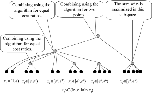
Figure 1: Schematic description of Combined.

We next describe a new algorithm, called Combined, defined on a UMTS $U=(\mathcal{U}^{d}_{b};r_{1},\dots,r_{b};s)$. This algorithm is inspired by Strategy 3 [3]. Like Strategy 3, Combined combines OddExponent and TwoStable on subspaces of $\mathcal{U}^{d}_{b}$, however, it does so in a more sophisticated way that is impossible using the combining technique of [3]. Fig. 1 presents the scheme of the combining process.

Algorithm Combined  As discussed in Observation 2.2, we may assume that $s=1$. Let $x_{i}$ be the minimal real number such that $r_{i}\leq 100\ln x_{i}\ln\ln x_{i}$ and $x_{i}\geq e^{e^{6}+1}$, and let $x$ denote $\sum_{i}x_{i}$. For a set $S\subset M^{d}_{b}$ let $U(S)$ denote the UMTS induced by $U$ on $S$.

Let $\mathcal{U}^{d}_{b}=\{v_{1},\ldots,v_{b}\}$, where $v_{i}$ has cost ratio $r_{i}$. We partition the points of $\mathcal{U}^{d}_{b}$ as follows: let $Q_{\ell}=\{v_{i}:\;e^{\ell-1}\leq x_{i}<e^{\ell}\}$. Let $P=\{Q_{\ell}:|Q_{\ell}|\geq\ln x\}\cup\{\{v\}:v\in Q_{\ell}\text{ and }|Q_{\ell}|<\ln x\}$, $P$ is a partition of $\mathcal{U}^{d}_{b}$. For $S\in P$ let $x(S)=\sum_{v_{i}\in S}x_{i}$. Without loss of generality we assume $P=\{S_{1},S_{2},\ldots,S_{b^{\prime}}\}$ where $b^{\prime}=|P|$ and $x(S_{j})\geq x(S_{j+1})$, $1\leq j\leq b^{\prime}-1$.

We associate with every set $S_{i}$ an algorithm $A(S_{i})$ on the UMTS $U(S_{i})$. If $|S_{i}|\geq\ln x$ we choose $A(S_{i})$ to be the $(1/10)$-variant of OddExponent. If $|S_{i}|<\ln x$ then $|S_{i}|=1$ and we choose $A(S_{i})$ to be the trivial algorithm on one point, this algorithm has a competitive ratio equal to the cost ratio, and it is $(0,0)$-constrained. Let $r(S_{i})$ denote the competitive ratio of $A(S_{i})$ on $U(S_{i})$.

If $b^{\prime}=1$ we choose Combined to be $A(S_{1})$ and we are done. If $b^{\prime}\geq 2$, let $\tilde{M}=\cup_{i=2}^{b^{\prime}}S_{i}$. We want to construct an algorithm, $A(\tilde{M})$, for $U(\tilde{M})$. If $b^{\prime}=2$, we choose $A(\tilde{M})$ to be $A(S_{2})$. Otherwise, we apply Theorem 3.1 on $\tilde{M}$ with the partition $\{S_{2},\ldots,S_{b^{\prime}}\}$. We define $\hat{M}$ from Theorem 3.1 to be $\mathcal{U}^{d}_{b^{\prime}-1}$. Likewise, $\hat{A}$ from Theorem 3.1 is the application of the $(1/5)$-variant of OddExponent on $\hat{U}=(\mathcal{U}^{d}_{b^{\prime}-1};r(S_{2}),\ldots,r(S_{b^{\prime}}))$. Let $r(\tilde{M})$ denote the competitive ratio of $\hat{A}$.

Next, we choose the partition $\{S_{1},\tilde{M}\}$ of $\mathcal{U}^{d}_{b}$. We combine the two algorithms $A(S_{1})$ and $A(\tilde{M})$ using the $(1/10)$ variant of TwoStable (this is the $\hat{A}$ required in Theorem 3.1) on the UMTS $(\mathcal{U}^{d}_{2};r(S_{1}),r(\tilde{M}))$ (the UMTS $\hat{U}$ of Theorem 3.1). We denote the competitive ratio of $\hat{A}$ by $r$. The resulting combined algorithm, $A(M)$, is our final algorithm, Combined.

Lemma 4.4.

Given that $x=\sum_{i}x_{i}$, $r_{i}\leq 100s\ln x_{i}\ln\ln x_{i}$, and $x_{i}\geq e^{e^{6}+1}$, algorithm Combined for the UMTS $U=(\mathcal{U}^{d}_{b};r_{1},$ $\ldots,r_{b};s)$ is $(1,1/2)$-constrained and $r$-competitive, where $r\leq 100s\ln x\ln\ln x$.

Proof.

As before, without loss of generality, we assume $s=1$. First we calculate the constraints of the algorithm.

From Lemma 4.1 and Lemma 3.11, $A(S_{i})$ is $(1/10,1/10)$-constrained, for every $1\leq i\leq b^{\prime}$. We would like to show that $A(\tilde{M})$ is $(1/2,3/10)$-constrained. If $b^{\prime}=2$ then it obviously $(1/10,1/10)$-constrained. Otherwise, ($b^{\prime}>2$), the combining algorithm for $\tilde{M}$ is the $(1/5)$-variant of OddExponent which is $(1/5,1/5)$-constrained. Hence, from (5), $\beta\leq 1/5+1/10+1/10+1/10=1/2$, and from (6), $\eta\leq 1/5+1/10=3/10$. From Corollary 3.2, $A(\tilde{M})$ is $r(\tilde{M})$ competitive.

The $(\beta,\eta)$-constraints of algorithm Combined are calculated as follows: The $(1/10)$-variant of TwoStable is $(1/10,2/10)$ constrained, therefore $\beta=1/10+1/10+1/2+3/10=1$ and $\eta=2/10+3/10=1/2$. From Corollary 3.2, $A(M)$ is $r$-competitive.

To summarize, Combined is $(1,1/2)$-constrained and $r$-competitive algorithm for the UMTS $U$.

It remains to prove the bound on $r$. First we show that $r(S_{j})\leq 100s\ln x(S_{j})\ln\ln x(S_{j})$ for all $1\leq j\leq b^{\prime}$. If $|S_{j}|=1$, we are done. Otherwise, $|S_{j}|\geq\ln x$, and $S_{j}=Q_{\ell}$ for some $\ell$.

$$r(S_{j}) \leq 100\ln e^{\ell}\ln\ln e^{\ell}+6\cdot 10\ln|S_{j}|$$ (20)

$$\leq 100\bigl{(}\ln e^{\ell-1}\ln\ln e^{\ell-1}+\ln\ell+\tfrac{1}{\ell-1}\ln e^{\ell-1}\bigr{)}+60\ln|S_{j}|$$

$$\leq 100\bigl{(}\ln e^{\ell-1}\ln\ln e^{\ell-1}+\ln\ln x+\tfrac{60}{100}\ln|S_{j}|+1\bigr{)}$$ (21)

$$\leq 100\bigl{(}\ln e^{\ell-1}\ln\ln e^{\ell-1}+2\ln|S_{j}|\bigr{)}$$ (22)

$$\leq 100\ln(|S_{j}|e^{\ell-1})\ln\ln(|S_{j}|e^{\ell-1})$$

$$\leq 100\ln x(S_{j})\ln\ln x(S_{j}).$$ (23)

Inequality (20) is derived as follows. Since $S_{j}=Q_{\ell}$, it follows that $r_{i}\leq 100s\ln e^{\ell}\ln\ln e^{\ell}$ for all $v_{i}\in S_{j}$. By the bound on the competitive ratio of the $(1/10)$ variant of OddExponent (See Lemma 4.1 and Lemma 3.11) we obtain (20). Inequality (21) follows since $\ell\leq\ln x$. Inequality (22) follows because $\ln|S_{j}|\geq\ln\ln x$, and $\ln\ln x\geq 6$. The last inequality follows because $e^{\ell-1}$ is a lower bound on $x_{i}$ for $v_{i}\in S_{j}$ and thus $|S_{j}|e^{\ell-1}\leq x(S_{j})$.

Observe that $b^{\prime}\leq\ln^{2}x$ as there are at most $\ln x$ sets $Q_{i}$, and each such set contributes at most $\ln x$ sets $S_{i}$ to $P$. We next derive a bound on $r(\tilde{M})$.

$$r(\tilde{M}) \leq \max_{2\leq i\leq b^{\prime}}r(S_{i})+6\cdot 5\cdot\ln(b^{\prime}-1)$$ (24)

$$\leq 100\cdot\ln x(S_{2})\ln\ln x+30\cdot(2\ln\ln x)$$

$$= 100(\ln x(S_{2})+0.6)\ln\ln x.$$

Inequality (24) follows since the algorithm used is a $(1/5)$ variant of OddExponent. Inequality (4) follows by using the previously derived bound on $r(S_{i})$ and noting that $x(S_{2})$ is maximal amongst $x(S_{2}),\ldots,x(S_{b^{\prime}})$ and that $x(S_{i})\leq x$.

From Lemma 3.11 we know that the competitive ratio of the $(1/10)$-variant of TwoStable is $f(10,r(S_{1}),r(\tilde{M}))$ where $f$ is the function as given in Proposition 4.3. We give an upper bound on $f(10,r(S_{1}),r(\tilde{M}))$ using Proposition 4.3. To do this we need to find values $y_{1}$ and $y_{2}$ such that

$$r(S_{1})\leq 100\ln x(S_{1})\ln\ln x =2\cdot 10(\ln y_{1}+1)$$

$$r(\tilde{M})\leq 100(\ln x(\tilde{M})+0.6)\ln\ln x =2\cdot 10(\ln y_{2}+1).$$

Indeed, the following values satisfy the conditions above: $y_{1}=x(S_{1})^{5\ln\ln x}/e$ and $y_{2}=(e^{0.6}x(\tilde{M}))^{5\ln\ln x}/e$. Using Proposition 4.3 we get a bound on $r$ as follows

$$r \leq 2\cdot 10(\ln(y_{1}+y_{2})+1)$$ (26)

$$\leq 20\ln\bigl{(}x(S_{1})^{5\ln\ln x}+(e^{0.6}x(\tilde{M}))^{5\ln\ln x}\bigr{)}$$

$$\leq 20\ln\bigl{(}x(S_{1})^{5\ln\ln x}+(2^{5\ln\ln x}-1)x(\tilde{M})^{5\ln\ln x}\bigr{)}$$ (27)

$$\leq 20\ln\bigl{(}(x(S_{1})+x(\tilde{M}))^{5\ln\ln x}\bigr{)}$$ (28)

$$\leq 100\ln x\ln\ln x.$$

Inequality (26) follows from Proposition 4.3. Inequality (27) follows because $\ln\ln x\geq 6$. Inequality (28) follows since, in general, for $a\geq b>0$ and $z\geq 1$, $a^{z}+(2^{z}-1)b^{z}\leq(a+b)^{z}$. This is because for $a=b$ it is an equality, and the derivative with respect to $a$ of the RHS is clearly larger than the derivative with respect to $a$ of the LHS. ∎

Next, we present a better algorithm when all the cost ratios but one are equal.

Lemma 4.5.

Given a UMTS $U=(\mathcal{U}^{d}_{b};r_{1},r_{2},\ldots,r_{b})$ with $r_{2}=r_{3}=\cdots=r_{b}$, there exists a $(1,3/5)$-constrained and $r$-competitive online algorithm, WCombined, where

$$r=30\Bigl{(}\ln\bigl{(}e^{\frac{r_{1}}{30}-\frac{1}{3}}+(b-1)e^{\frac{r_{2}}{30}-\frac{1}{3}}\bigr{)}+\tfrac{1}{3}\Bigr{)}.$$

Proof.

The proof is a simplified version of the proof of Lemma 4.4, and we only sketch it here. We define $x_{1}$, $x_{2}$, such that

$$r_{1} =30(\ln x_{1}+\tfrac{1}{3})=2\cdot 5\cdot(\ln x_{1}^{3}+1), r_{2} =30(\ln x_{2}+\tfrac{1}{3})=2\cdot 5\cdot(\ln x_{2}^{3}+1).$$

Let $\tilde{M}=\{v_{2},\ldots v_{b}\}$. We use a $(1/5)$ variant of OddExponent on the UMTS $U(\tilde{M})$. The competitive ratio of this algorithm is at most

$$r(\tilde{M})\leq r_{2}+30\ln(b-1)\leq 30\bigl{(}\ln((b-1)x_{2})+\tfrac{1}{3}\bigr{)}=10\bigl{(}\ln((b-1)x_{2})^{3}+1\bigr{)}$$

and it is $(1/5,1/5)$ constrained. We combine it with the trivial algorithm for $U(\{v_{1}\})$ using a $(1/5)$ variant of algorithm TwoStable, the resulting algorithm is $(1,3/5)$ constrained, and by Proposition 4.3 we have

$$r\leq 10(\ln(x_{1}^{3}+((b-1)x_{2})^{3}+1)\leq 10(\ln(x_{1}+(b-1)x_{2})^{3}+1)=30(\ln(x_{1}+(b-1)x_{2})+\tfrac{1}{3}).$$

Substituting for $x_{i}$ gives the required bound. ∎

5 Applications

5.1 An ${O((\log n\log\log n)^{2})}$ Competitive algorithm for MTSs

Bartal [1] defines a class of decomposable spaces called hierarchically well separated trees (HST).

Definition 5.1.

For $k\geq 1$, a $k$-hierarchically well-separated tree ($k$-HST) is a metric space defined on the leaves of a rooted tree $T$. Associated with each vertex $u\in T$ is a real valued label $\Delta(u)\geq 0$, and $\Delta(u)=0$ if and only if $u$ is a leaf of $T$. The labels obey the rule that for every vertex $v$, a child of $u$, $\Delta(v)\leq\Delta(u)/k$. The distance between two leaves $x,y\in T$ is defined as $\Delta(\operatorname{lca}(x,y))$, where $\operatorname{lca}(x,y)$ is the least common ancestor of $x$ and $y$ in $T$. Clearly, this is a metric.

Bartal [1, 2] shows how to approximate any metric space using an efficiently constructible probability distribution over a set of $k$-HSTs . His result allows to reduce a MTS problem on an arbitrary metric space to MTS problems on HSTs. Formally, he proves the following theorem.

Theorem 5.2 ([2]).

Suppose there is a $r$-competitive algorithm for any $n$-point $k$-HST metric space. Then there exists an $O(rk\log n\log\log n)$-competitive randomized algorithm for any $n$-point metric space.

Thus, it is sufficient to construct an online algorithm for a metrical task system where the underlying metric space is a $k$-HST. Following [3] we use the unfair MTS model to obtain an online algorithm for a MTS over a $k$-HST metric space.

Algorithm Rhst.  We define the algorithm Rhst($T$) on the metric space $M(T)$, where $T$ is a $k$-HST with $k\geq 5$. Algorithm Rhst($T$) is defined inductively on the size of the underlying HST, $T$.

When $|M(T)|=1$, Rhst($T$) serves all task sequences optimally. It is $(0,0)$-constrained. Otherwise, let the children of the root of $T$ be $v_{1},\ldots,v_{b}$, and let $T_{i}$ be the subtree rooted at $v_{i}$. Denote $d=\Delta(T)$, and so $\operatorname{diam}(T_{i})\leq d/k$. Every algorithm Rhst($T_{i}$) is an algorithm for the UMTS $U_{i}=(M(T_{i});1,\ldots,1;1)$.

We construct a metric space $\hat{M}=\mathcal{U}^{d}_{b}$, and define cost ratios $r_{1},\ldots,r_{b}$ where $r_{i}=r(T_{i})$ is the competitive ratio of Rhst($T_{i}$). We now use Theorem 3.1 to combine algorithms Rhst($T_{i}$). The role of $\hat{A}$ is played by the $(1/2)$ variant of Combined on the unfair metrical task system $\hat{U}=(\hat{M};r_{1},\ldots,r_{b};1)$. The combined algorithm is a Rhst($T$) on the UMTS $(M(T);1,\ldots,1;1)$.

We remark that the application of Theorem 3.1 requires that the algorithms will be constrained. We show that this is true in the following lemma.

Lemma 5.3.

The algorithm Rhst($T$) is $O(\ln n\ln\ln n)$, where $n=|M(T)|$.

Proof.

Let $n^{\prime}=e^{e^{6}+1}n$. We prove by induction on the depth of the tree that Rhst($T$) is $(1,1)$-constrained and $200\ln n^{\prime}\ln\ln n^{\prime}$-competitive.

When $|M(T)|=1$, it is obvious. Otherwise, let $n_{i}=|M(T_{i})|$, $n^{\prime}_{i}=e^{e^{6}+1}n_{i}$, and $n^{\prime}=\sum_{i}n^{\prime}_{i}$. We assume inductively that each of the Rhst($T_{i}$) algorithms is $(1,1)$-constrained and $200\ln n^{\prime}_{i}\ln\ln n^{\prime}_{i}$ competitive on $M(T_{i})$. The combined algorithm, Rhst($T$), is $(\beta,\eta)$-constrained. From (5), and given that $k\geq 5$, we get that

$$\beta\leq\max\{1,\tfrac{1}{2}+\tfrac{1}{k}+\tfrac{1}{k}+\tfrac{1}{2k}\}\leq\max\{1,1\}=1.$$

From (6) we obtain that $\eta\leq\tfrac{1}{2}+\tfrac{1}{k}\leq 1$, for $k\geq 5$. This proves that the algorithm is well defined and $(1,1)$ constrained.

We next bound the competitive ratio using Lemma 4.4. Lemma 3.11 implies that the competitive ratio obtained by the $(1/2)$ variant of Combined on $(\hat{M};r_{1},\ldots,r_{b})$ is the same as the competitive ratio attained by Combined on $(\hat{M};r_{1},\ldots,r_{b};2)$. The values $(x_{i})_{i}$ computed by Combined are at most $(n^{\prime}_{i})_{i}$, respectively. Hence it follows from Lemma 4.4 that the competitive ratio of Rhst($T$) is at most $100\cdot 2\ln x\ln\ln x\leq 200\ln n^{\prime}\ln\ln n^{\prime}$, since $x=\sum_{i}x_{i}$. ∎

Since every HST $T$ can be $5$-approximated by a 5-HST $T^{\prime}$ (see [2]), the bound we have just proved holds for any HST.

Combining Theorem 5.2 with Lemma 5.3, it follows that

Theorem 5.4.

For any MTS over an $n$-point metric space, the randomized competitive ratio is $O((\log n\log\log n)^{2})$.

5.2 $K$-Weighted Caching on $K+1$ Points

Weighted caching is a generalized paging problem where there is a different cost to fetch different pages. This problem is equivalent to the $K$-server problem on a star metric space [21, 9]. A star metric space is derived from a depth one tree with distances on the edges, the points of the metric space are the leaves of the tree and the distance between a pair of points is the length of the (2 edge) path between them. This is so, since we can assign any edge $(r,u)$ in the tree a weight of half the fetch cost of $u$. Together, an entrance of a server into a leaf from the star’s middle-point (page in) and leaving the leaf to the star’s middle point (page out) have the same cost of fetching the page.

The $K$-server problem on a metric space of $K+1$ points is a special case of the metrical task system problem on the same metric space, and hence any upper bound for the metrical task system translates to an upper bound for the corresponding $K$-server problem.

Given a star metric space $M$, we $12$-approximates it with a $6$-HST $T$. $T$ has the special structure that for every internal vertex, all children except perhaps one, are leaves. It is not hard to see that one can find such a tree $T$ such that for any $u,v\in M$, $\operatorname{d}_{M}(u,v)\leq\operatorname{d}_{T}(u,v)\leq 12\cdot\operatorname{d}_{M}(u,v).$ Essentially, the vertices furthest away from the root (up to a factor of 6) in the star are children of the root of $T$ and the last child of the root is a recursive construction for the rest of the points.

We now follow the construction of Rhst given in the previous section, on an 6-HST $T$, except that we make use of $(1/2)$-variant of WCombined rather than $(1/2)$-variant of Combined. The special structure of $T$ implies that all the children of an inner vertex, except perhaps one, are leaves and therefore have a trivial $1$-competitive algorithm on their “subspaces”. Hence we can apply WCombined. Using Lemma 4.5 with induction on the depth of the tree, it is easy to bound the competitive ratio on $K+1$ leaves tree to be at most $60(\ln(K+1)+1/3)$.

Combining the above with the lower bound of [9] we obtain:

Theorem 5.5.

The competitive ratio for the $K$-weighted caching problem on $K+1$ points is $\Theta(\log K)$.

5.3 A MTS on Equally Spaced Points on the Line

The metric space of $n$ equally spaced points on the line is considered important because of its simplicity, and the practical significance of the $k$-server on the line (for which this problem is a special case). The best lower bound currently known on the competitive ratio is $\Omega(\log n/\log\log n)$ [10]. Previously, the best upper bound known was $O(\log^{3}n/\log\log n)$ due to [3].

We are able to slightly improves the upper bound on the competitive ratio from Section 5.1 to $O(\log^{2}n)$. Bartal [1] proves that $n$ equally spaced points on the line can be $O(\log n)$ probabilistically embedded into a set of binary $4$-HSTs. We present an $O(\log n)$ competitive randomized algorithm for binary $4$-HST, similar to Rhst except that we make use of $(1/4)$-variant of TwoStable instead of $(1/2)$-variant of Combined. Similar arguments show that this algorithm is $(1,1)$-constrained, and using Proposition 4.3 we conclude that the algorithm is $8\ln n$ competitive. Combining the probabilistic embedding into binary $4$-HST with the algorithm for binary $4$-HST we obtain

Theorem 5.6.

The competitive ratio of the MTS problem on metric space of $n$ equally spaced points on the line is $O(\log^{2}n)$.

6 Concluding Remarks

This paper present algorithms for MTS problem and related problems with significantly improved competitive ratios. An obvious avenue of research is to further improve the upper bound on the competitive ratio for the MTS problem. A slight improvement to the competitive ratio of the algorithm for arbitrary $n$-point metric spaces is reported in [6]. The resulting competitive ratio there is $O(\log^{2}n\log\log n\log\log\log n)$ and the improvement is achieved by refining the reduction from arbitrary metric spaces to HST spaces (i.e., that improvement is orthogonal to the improvement presented in this paper). However, in order to break the $O(\log^{2}n)$ bound, it seems that one needs to deviate from the black box usage of Theorem 5.2. Maybe the easiest special case to start with is the metric space of equally spaced points on the line.

Another interesting line of research would be an attempt to apply the techniques of this and previous papers to the randomized $k$-server problem, or even for a special case such as the randomized weighted caching on $k$ pages problem; see also [8, 19].

Acknowledgments

We would like to thank Yair Bartal, Avrim Blum and Steve Seiden for helpful discussions.

References

- [1] Y. Bartal, Probabilistic approximation of metric space and its algorithmic application, in 37th Annual Symposium on Foundations of Computer Science, Oct. 1996, pp. 183–193.
- [2] , On approximating arbitrary metrics by tree metrics, in Proceedings of the 30th Annual ACM Symposium on Theory of Computing, 1998, pp. 183–193.
- [3] Y. Bartal, A. Blum, C. Burch, and A. Tomkins, A polylog()-competitive algorithm for metrical task systems, in Proceedings of the 29th Annual ACM Symposium on Theory of Computing, May 1997, pp. 711–719.
- [4] Y. Bartal, B. Bollobás, and M. Mendel, A ramsey-type theorem for metric spaces and its application for metrical task systems and related problems, in Proceedings of the 42nd Annual Symposium on Foundations of Comptuer Science, Las Vegas, Nevada, 2001.
- [5] Y. Bartal, N. Linial, M. Mendel, and A. Naor, On metric ramsey-type phenomena, in Proc. 35th ACM Symposium on the Theory of Computing, 2003.
- [6] Y. Bartal and M. Mendel, Multi-embeddings and path-approximation of metric spaces, in 14th Ann. ACM-SIAM Symposium on Discrete Algorithms, 2003.
- [7] S. Ben-David, A. Borodin, R. Karp, G. Tardos, and A. Wigderson, On the power of randomization in on-line algorithms, Algorithmica, 11 (1994), pp. 2–14.
- [8] A. Blum, C. Burch, and A. Kalai, Finely-competitive paging, in 40th IEEE Symposium on Foundations of Computer Science, 1999.
- [9] A. Blum, M. L. Furst, and A. Tomkins, What to do with your free time: algorithms for infrequent requests and randomized weighted caching. manuscript, Apr. 1996.
- [10] A. Blum, H. Karloff, Y. Rabani, and M. Saks, A decomposition theorem and lower bounds for randomized server problems, SIAM J. Comput., 30 (2000), pp. 1624–1661.
- [11] A. Borodin, N. Linial, and M. Saks, An optimal online algorithm for metrical task systems, J. Assoc. Comput. Mach., 39 (1992), pp. 745–763.
- [12] M. Chrobak, H. Karloff, T. Payne, and S. Vishwanathan, New results on server problems, in 1st Annual ACM-SIAM Symposium on Discrete Algorithms, 1990, pp. 291–300.
- [13] M. Chrobak and L. L. Larmore, The server problem and on-line games, in On-line Algorithms, L. A. McGeoch and D. D. Sleator, eds., vol. 7 of DIMACS Series in Discrete Mathematics and Theoretical Computer Science, Feb. 1991, pp. 11–64.
- [14] S. Irani and S. Seiden, Randomized algorithms for metrical task systems, Theoretical Computer Science, 194 (1998), pp. 163–182.
- [15] A. Karlin, M. Manasse, L. Rudolph, and D. D. Sleator, Competitive snoopy caching, Algorithmica, 3 (1988), pp. 79–119.
- [16] H. Karloff, Y. Rabani, and Y. Ravid, Lower bounds for randomized -server and motion-planning algorithms, SIAM Journal on Computing, 23 (1994), pp. 293–312.
- [17] M. Manasse, L. A. McGeoch, and D. Sleator, Competitive algorithms for server problems, Journal of Algorithms, 11 (1990), pp. 208–230.
- [18] S. Seiden, Unfair problems and randomized algorithms for metrical task systems, Information and Computation, 148 (1999), pp. 219–240.
- [19] , A general decomposition theorem for the -server problem, in 9th Annual European Symposium on Algorithms, vol. 2161 of LNCS, Springer, 2001, pp. 86–97.
- [20] D. D. Sleator and R. E. Tarjan, Amortized efficiency of list update and paging rules, Communication of the ACM, 28 (1985), pp. 202–208.
- [21] N. E. Young, The k-server dual and loose competitiveness for paging, Algorithmica, 11 (1994), pp. 525–541.