*

Abstract

We discuss online strategies for visibility-based searching for an object hidden behind a corner, using Kurt3D, a real autonomous mobile robot. This task is closely related to a number of well-studied problems. Our robot uses a three-dimensional laser scanner in a stop, scan, plan, go fashion for building a virtual three-dimensional environment. Besides planning trajectories and avoiding obstacles, Kurt3D is capable of identifying objects like a chair. We derive a practically useful and asymptotically optimal strategy that guarantees a competitive ratio of 2, which differs remarkably from the well-studied scenario without the need of stopping for surveying the environment. Our strategy is used by Kurt3D, documented in a separate video.

Keywords: Searching, visibility problems, watchman problems, online searching, competitive strategies, autonomous mobile robots, three-dimensional laser scanning, Kurt3D.

1 Introduction

Visibility Problems. Visibility-based problems of surveying, guarding, or searching have a long-standing tradition in the area of computational optimization; they may very well be considered a field of their own. Using stationary positions for guarding a region is the well-known art gallery problem [o-agta-87]. The watchman problem [thi-iacsw-93, thi-ciacs-99, cjn-fswrsp-99] asks for a short tour along which one mobile guard can see the entire region. If the region is unknown in advance, we are faced with the online watchman problem. For a simple polygon, Hoffmann et al.[hikk-pep-01] achieve a constant competitive ratio of 26.5, while Albers et al. [aks-eueo-99] show that no constant competitive factor exists for a region with holes, and unbounded aspect ratio. Kalyanasundaram and Pruhs [kp-cctli-94] consider the problem in graphs and give a competitive factor of 18.

In the context of geometric searching, a crucial issue is the question of how to look around a corner: Given a starting position, and a known distance to a corner, how should one move in order to see a hidden object (or the other part of the wall) as quickly as possible? This problem was solved by Icking et al.[ikm-hlac-93, ikm-ocsla-94] who show that an optimal strategy can be characterized by a differential equation that yields a competitive factor of 1.2121…, which is optimal. It should be noted that actually using this solution requires numerical evaluation.

An Autonomous Mobile Robot. From the practical side, our work is motivated by an actual application in robotics: The Fraunhofer Institute for Autonomous Intelligent Systems (AIS) has developed autonomous mobile robots that can survey their environment by virtue of a high-resolution, 3D laser scanner [RAAS2003]. By merging several 3D scans acquired in a stop, scan, plan, go fashion, the robot Kurt3D builds a virtual 3D environment that allows it to navigate, avoid obstacles, and detect objects[IAS2004]. This makes the visibility problems described above quite practical, as actually using good trajectories is now possible and desirable.

However, while human mobile guards are generally assumed to have full vision at all times, our autonomous robot has to stop and take some time for taking a survey of its environment. This makes the objective function (minimize total time to locate an object or explore a region) a sum of travel time and scan time; a somewhat related problem is searching for an object on a line in the presence of turn cost [dfg-ostc-04], which turns out to be a generalization of the classical linear search problem. Somewhat surprisingly, scan cost (however small it may be) causes a crucial difference to the well-studied case without scan cost, even in the limit of infinitesimally small scan times.

Other Related Work. Visbility-based navigation of robots involves a variety of different aspects. For example, Efrat et al. [egkp-ostcpt-03] study the task of developing strategies for tracking and capturing a visible target with known trajectory, while maintaining line-of-sight among obstacles. Kutulakos et al. [kdl-psvgetd-94] consider the task of vision-guided exploration, where the robot is assumed to move about freely in three dimensions, among various obstacles.

Our Results. The main objective of this paper is to demonstrate that technology has reached the stage of actually applying previous theoretical studies, at the same time triggering new algorithmic research. We hope that this will highlight the need for and the opportunities of closer interaction between theoreticians and practitioners. In particular, we describe the problem of online searching by a real autonomous robot, for an object (a chair) hidden behind a corner, which is at distance $d$ from the robot’s starting position. Our mathematical results are as follows:

• We show that for an initial distance of at least $d\geq 1/\delta$ from the corner, a competitive ratio of $2-\delta$ cannot be achieved. This implies a lower bound of 2 on the competitive ratio by any one strategy, and proves that there is an important distinction from the case without scan cost.

• We describe a heuristic strategy that is fast to evaluate and easy to implement in real life.

• We show that this strategy is asymptotically optimal by proving that for large distances, the competitive ratio converges to 2, matching the lower bound.

• We give additional numerical evidence showing that the performance of our strategy is within about 2% of the optimum.

• Most importantly, we describe how our strategy can actually be used by Kurt3D, a real mobile autonomous robot.

Further documentation of our work is provided by a video [fkn-sarv-04] that is available at the authors’ web address.

The rest of this paper is organized as follows. In Section 2, we describe the technical details, properties, and capabilities of Kurt3D, an autonomous mobile robot that was used in our experiments. Section 3 provides mathematical results on the problem arising from Kurt searching for a hidden object. Section 4 gives a description of how our results are used in practice. The final Section 5 provides some directions for future research.

2 The Autonomous Mobile Robot

2.1 The Kurt3D Robot Platform

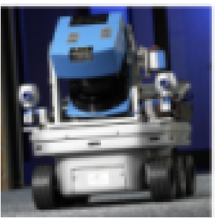
Kurt3D (Figure 1, top left) is a mobile robot platform with a size of 45 cm (length) $\times$ 33 cm (width) $\times$ 26 cm (height) and a weight of 15.6 kg. Equipped with the 3D laser range finder the height increases to 47 cm and the weight to 22.6 kg. Kurt3D’s maximum velocity is 5.2 m/s (autonomously controlled 4.0 m/s). Two 90 W motors are used to power the 6 wheels, where the front and rear wheels have no tread pattern to enhance rotating. Kurt3D operates for about 4 hours with one battery (28 NiMH cells, capacity: 4500 mAh) charge. The core of the robot is a Pentium-III-600 MHz with 384 MB RAM. An embedded 16-Bit CMOS microcontroller is used to control the motor.

2.2 The AIS 3D Laser Range Finder

The AIS 3D laser range finder (Figure 1, top right) [RAAS2003, ISR2001] is built on the basis of a 2D range finder by extension with a mount and a standard servo motor. The 2D laser range finder is attached in the center of rotation to the mount for achieving a controlled pitch motion. The servo is connected on the left side (Figure 1, top middle). The 3D laser scanner operates up to 5h (Scanner: 17 W, 20 NiMH cells with a capacity of 4500 mAh, Servo: 0.85 W, 4.5 V with batteries of 4500 mAh) on one battery pack.

Figure 1: Top left: The autonomous mobile robot Kurt3D equipped with the 3D scanner. Top right: The AIS 3D laser range finder. Its technical basis is a SICK 2D laser range finder (LMS-200). Bottom row, left: A scanned scene as depth image. Middle and right: Scanned scenes as point cloud viewed with a camera orientation towards the door.

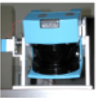
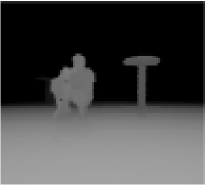
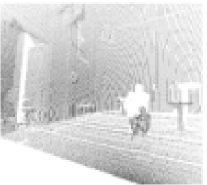
The area of $180^{\circ}\mbox{(h)}\times 120^{\circ}\mbox{(v)}$ is scanned with different horizontal (181, 361, 721 pts.) and vertical (210, 420 pts.) resolutions. A plane with 181 data points is scanned in 13 ms by the 2D laser range finder (rotating mirror device). Planes with more data points, e.g., 361, 721, duplicate or quadruplicate this time. Thus, a scan with 181 $\times$ 210 data points needs 2.8 seconds. In addition to the distance measurement, the 3D laser range finder is capable of quantifying the amount of light returning to the scanner, i.e., reflectance data [IAS2004]. Figure 1 (bottom left) shows a scanned scene as depth image, created by off-screen rendering from the 3D data points (Figure 1, bottom middle) by an OpenGL-based drawing module.

2.3 Basic 3D Scanner Software

The basis of the scan matching algorithms and the reliable robot control are algorithms for reducing points, line detection, surface extraction and object segmentation. Next we give a brief description of these algorithms. Details can be found in [ISR2001].

The scanner emits the laser beams in a spherical way, such that the data points close to the source are more dense. The first step is to reduce the data. Therefore, data points located close together are joined into one point. The number of these so-called reduced points is one order of magnitude smaller than the original one.

Second, a simple length comparison is used as a line detection algorithm. Given that the counterclockwise ordered data of the laser range finder (points $a_{0},a_{1},\ldots,a_{n}$) are located on a line, the algorithm has to check for $a_{j+1}$ if $\|a_{i},a_{j+1}\|\ /\ \sum^{j}_{t=i}\|a_{t},a_{t+1}\|<\epsilon(j)$ in order to determine if $a_{j+1}$ is on line with $a_{j}$. (Figure 2, left)

The third step is surface detection. Scanning a plane surface, line detection returns a sequence of lines in successive scanned 2D planes approximating the shape of surfaces. Thus a plain surface consists of a set of lines. Surfaces are detected by merging similar oriented and nearby lines. (Figure 2, middle)

The fourth and final step computes occupied space. For this purpose, conglomerations of surfaces and polygons are merged sequentially into objects. Two steps are necessary to find bounding boxes around objects. First a bounding box is placed around each large surface. In the second step objects close to each other are merged together, e.g., one should merge objects closer than the size of the robot, since the robot cannot pass between such objects (Figure 2, right). These bounding boxes are used for avoiding obstacles.

Data reduction, line, surface and object detection are real-time capable and run in parallel to the 3D scanning process.

Figure 2: Left: Line detection in every scan slice. Middle: Surface segmentation. Right: Bounding boxes of objects superimposing the surfaces

2.4 3D Scan Matching

To create a correct and consistent representation of the environment, the acquired 3D scans have to be merged in one coordinate system. This process is called registration. Due to the robot’s sensors, the self-localization is usually erroneous and imprecise, so the geometric structure of overlapping 3D scans has to be considered for registration. The odometry-based robot pose serves as a first estimate and is corrected and updated by the registration process. We use the well-known Iterative Closest Points (ICP) algorithm [Besl_1992] to compute the transformation, consisting of a rotation $\mathbf{R}\in\mathbbm{R}^{3\times 3}$ and a translation $\mathbf{t}\in\mathbbm{R}^{3}$. The ICP algorithm computes this transformation in an iterative fashion. In each iteration the algorithm selects the closest points as correspondences and computes the transformation ($\mathbf{R},\mathbf{t}$) for minimizing

$$E(\mathbf{R},\mathbf{t})\!=\!\sum_{i=1}^{N_{m}}\sum_{j=1}^{N_{d}}w_{i,j}\left|\left|\mathbf{m}_{i}-(\mathbf{R}\mathbf{d}_{j}+\mathbf{t})\right|\right|^{2},$$

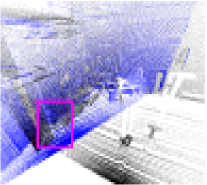
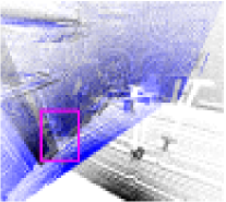
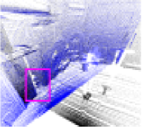
where $N_{m}$ and $N_{d}$ are the number of points in the model set $M$, i.e., first 3D scan, or data set $D$, second 3D scan, respectively, and $w_{ji}$ are the weights for a point match. The weights are assigned as follows: $w_{ji}=1$, if $\mathbf{m}_{i}$ is the closest point to $\mathbf{d}_{j}$ within a close limit, $w_{ji}=0$ otherwise. It is shown in [Besl_1992] that the iteration terminates in a minimum. The assumption is that in the last iteration the point correspondences are correct. In each iteration the transformation is computed in a fast closed-form manner by the quaternion-based method of Horn [Horn_1987]. In addition, point reduction and $k$D.trees speed up the computation of the point pairs, such that only the time required for scan matching is reduced to roughly one second [RAAS2003]. Figure 3 shows three iteration steps for 3D scan alignment.

Figure 3: Three iteration steps of scan alignment process for the two 3D scans presented in Figure 1 (bottom, middle, right).

2.5 3D Object Detection

[0,r, ,Object detection in range images.] Automatic, fast and reliable object detection algorithms are essential for mobile robots used in searching tasks. To perceive objects, we use the 3D laser range and reflectance data. The 3D data is transformed into images by off-screen rendering. To detect objects, a cascade of classifiers, i.e., a linear decision tree, is used. Following the ideas of Viola and Jones, we compose each classifier from several simple classifiers, which in turn contain an edge, line or center surround feature [Viola_2001]. There exists an effective method for the fast computation of these features using an intermediate representation, namely, integral image. For learning of the object classes, a boosting technique, namely, Ada Boost, is used [Viola_2001]. The resulting approach for object classification is reliable and real-time capable and combines recent results in computer vision with the emerging technology of 3D laser scanners. For a detailed discussion of object detection in 3D laser range data, refer to [IAS2004]. Figure 2.5 shows an office chair detected by a cascade of classifiers.

3 Algorithmic Approach

When trying to develop a good search strategy, we have to balance theoretical quality with practical applicability. More precisely, we have to keep a close eye on the trade-off between these objectives: An increase in theoretical quality may come at the expense of higher mathematical difficulty, possibly requiring more complicated tools. In an online context, the use of such tools may cause both theoretical and practical difficulties: Complicated solutions may cause computational overhead that can change the solution itself by causing extra delay; on the practical side, actually applying such a solution may be difficult (due to limited accuracy of the robot’s motion) and without significant use. To put relevant error bounds into perspective: The largest room available to us is the great hall of Schloss Birlinghoven; even there, the size of Kurt and the object is still in the order of 2% of the room diameter.

On the mathematical side, it should be noted that even in the theoretical paper [hikk-pep-01], semi-circles are considered instead of the solution to the differential equation, in order to allow analysis of the resulting trajectories.

In the following, we will start by giving some basic mathematical observations and properties (Section 3.1); this is followed by a discussion of globally optimal strategies (Section 3.2). Section  3.3 describes a natural heuristic solution that is both easy to describe and fast to evaluate; we give a number of computational and empirical results that suggest our heuristic is within 2% of an optimal strategy. Finally, Section  3.4 provides a number of mathematical results, showing that our fast and easy heuristic is asymptotically optimal.

3.1 Basic Observations

First, we introduce some notation that will be used throughout this section.

Let us assume that the corner that hides the object is at distance $d$ from the start. Let $x_{i}$ denote the distance the robot travels in the $i-$th step, i.e., on its way from position $i-1$ to position $i$, from which the $i-$th scan will be taken. If the object was hidden infinitesimally behind position $i$, the optimal solution would go perpendicularly to the line $L_{i}$ that runs from the corner through position $i$, and then take one scan from there. Let $d_{i}$ denote the length of this line segment (observe that it meets $L_{i}$ at a point that lies on the semi-circle spanned by the start and the corner). Then the optimum cost to detect the object would be $1+d_{i}$, whereas the robot would only see the object at position $i+1$, having accumulated a cost of

$$i+1+\sum_{j=1}^{i+1}x_{j}.$$

Now suppose that $c$ is the smallest competitive ratio that can be achieved in this setting. By local optimality, for any scan position, the ratio of the solution achieved and the optimal solution must be equal to $c$. Therefore,

$$x_{i+1}=c(1+d_{i})-(i+1)-\sum_{j=1}^{i}x_{j}$$ (1)

must hold for $i=1,2,\ldots$ In particular, we have $x_{1}=c-1$ for the first step.

3.2 Globally Optimal Strategies

The above recursion can be used for proving a lower bound.

Theorem 3.1.

There is no global $c$-competitive strategy with $c<2$.

Proof 3.2.

Assume the claim was false, and there was a $c$-competitive strategy for $c=2-\delta$. We show that $x_{i}\leq(1-\delta)^{i}$ holds, making it impossible for the robot to get further than a distance of $1/\delta$ away from the start, a contradiction. Clearly, we have $x_{1}=1-\delta$ for step 1. Moreover,

$$d_{i}\leq\sum_{j=1}^{i}x_{j}$$

holds, because $d_{i}$ is the shortest path from the start to line $L_{i}$, whereas the sum denotes the length of the robot’s path. Plugging this into our recursion yields

$$x_{i+1}\leq(1-\delta)(1+\sum_{j=1}^{i}x_{j})-i.$$

By induction, we have $x_{j}\leq(1-\delta)^{j}$, hence

$$x_{i+1}\leq(1-\delta)\frac{1-(1-\delta)^{i+1}}{\delta}-i\leq(1-\delta)^{i+1},$$

using the Bernoulli inequality $1-(1+i)\delta\leq(1-\delta)^{i+1}$. ∎

Instead of increasing the distance $d$ we could as well consider a situation where start and corner are a distance 1 apart, but the scan cost is only $1/d$. Now Theorem 3.1 shows a remarkable discontinuity: Even for a scan cost arbitrarily small, a lower bound of 2 cannot be beaten, whereas for zero scan cost, a factor of $1.212\dots$ can be obtained [ikm-hlac-93].

On the positive side, for $n$ intermediate scan points, Equation (1) provides $n$ optimality conditions. As there are $2n$ degrees of freedom (the coordinates of intermediate scan points), we get an underdetermined nonlinear optimization problem for any given distance $d$, provided that we know the number of scan points. For $d=1$, this can be used to derive an optimal competitive factor of 1.808201…, achieved with one intermediate scan point. For larger $d$ (and hence, larger $n$) one could derive additional geometric optimality conditions and use them in combination with more complex numerical methods. However, this approach appears impractical for real applications, for reasons stated above. As we will see in the following, there is a better approach.

3.3 A Simple Heuristic Strategy

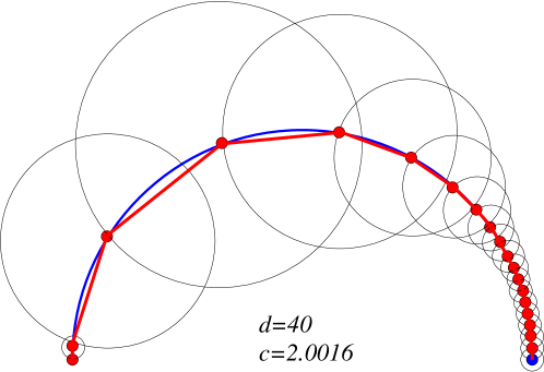
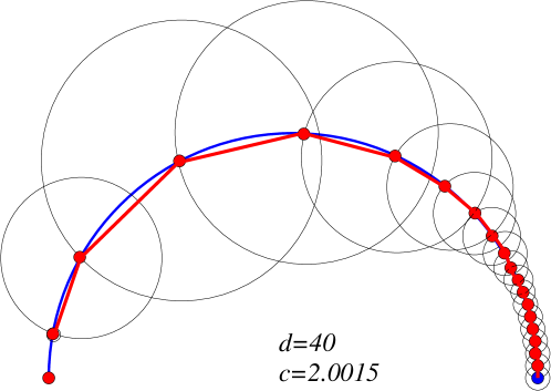
Now we describe a simple strategy for the searching problem that uses trajectories inscribed into a circle. This reduces the degrees of freedom to the point where evaluation is fast and easy. What is more, it works very well in realistic settings, and it is asymptotically optimal for decreasing cost of scanning, or growing size of the environment.

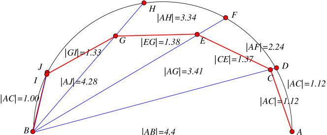
The robot simply follows a polygonal path inscribed into the semi-circle of diameter $d$, spanned by start and corner. It remains to determine those points where it stops for scanning its environment. This is done by applying the optimality condition derived in Section 3.1. In step $j$, the robot moves along a chord of length $x_{j}$. From the corner, this chord is visible under an angle of $\varphi_{j}=\arcsin(x_{j}/d)$. The chord connecting the start to position $i$ is of length

$$d_{i}=d\ \sin(\sum_{j=1}^{i}\varphi_{j}),$$

so that the recursion (1) obtained in Section 3.1 turns into

$$x_{i+1} = c\left(1+d\ \sin\left(\sum_{j=1}^{i}\arcsin\left(\frac{x_{j}}{d}\right)\right)\right)-(i+1)-\sum_{j=1}^{i}x_{j}.$$

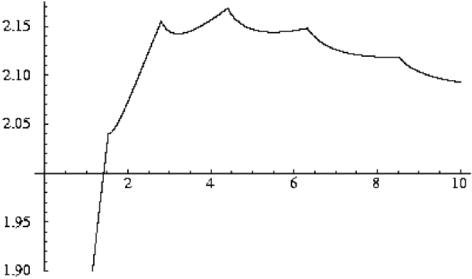
Given any $c>1$, we can tentatively compute steps of length $x_{i}$ by this formula, starting with $x_{1}=c-1$. If the resulting sequence reaches the corner, the ratio of $c$ can indeed be achieved. If it collapses prematurely (by returning negative values) $c$ was too small. (For example, $c=2.001525...$ is optimal for $d=40$; see Figure 4 for an illustration of upper and lower bounds on this value.)

Figure 4: An example for $d=40$: (top) For $c=2.0016$, the circle sequence reaches the corner, showing that the chosen $c$ can be achieved. (bottom) For $c=2.0015$, the sequence collapses before reaching the corner, showing that the chosen $c$ cannot be achieved. The actual optimum is about 2.001525…

By performing a binary search, the optimal ratio and the necessary step lengths can be computed extremely fast. Moreover, an analysis of the optimal ratio as a function of $d$ shows that a maximum is reached for $d=4.400875...$ which is precisely at the threshold between three and four necessary scans, with a competitive ratio of 2.168544. (See Table 1 for an overview of the critical values for which the number of scans increases, and Figure 6 for the achievable ratios as a function of the distance.) This is still within about 2% of the global optimum, which appears to be at about 2.12 (see Figure 5.) Moreover, numerical evidence shows that the ratio approaches 2 quite rapidly as $d$ tends to infinity. This is all the more surprising, as the resulting initial step length converges to 1, while a constant step length of 1 yields a competitive ratio of $\pi$. In the following Section 3.4 we give a mathematical proof of this observation.

Number	Maximal	$c$ at
of scans	$d$	upper bound
0	0.618034	1.618034
1	1.530414	2.040287
2	2.799395	2.155363
3	4.400876	2.168544
4	6.316892	2.147994
5	8.514200	2.118498

Table 1: Threshold values for small numbers of scans, rounded to six digits.

Figure 5: A solution for $d=4.4$ that achieves competitive ratio 2.12: The starting position is at $A$, the corner at $B$.

Figure 6: The competitive ratio as a function of $d$: (top) for small values of $d$; (bottom) for larger values of $d$; note the cusps at threshold values, the sharp peak at about (4.4,2.17), and the clear asymptotic behavior. The first step length, $x_{1}$ is given by $c-1$.

3.4 Asymptotics

As we have seen in Theorem 3.1, there is a lower bound of 2 on the competitive ratio for all strategies and large $d$. In the following we will show that for large $d$, there is a matching upper bound on our circle strategy presented in Section 3.3, proving it to be asymptotically optimal. For limited physical distances, it shows that even for arbitrarily small scan times, there is a relatively simple strategy that achieves the optimal ratio of 2.

Our proof of the upper bound proceeds as follows. Let us assume that we are given some fixed $\varepsilon>0$. We then proceed to show that for $c=2+\varepsilon$, the recursion presented in Section 3.3 does not collapse before the corner is reached, if the diameter $d$ of the semi-circle is large enough.

In proving the lower bound stated in Theorem 3.1, we have used the obvious fact that the length $d_{n}$ of the optimal path cannot exceed the length of the robot’s path. Now we are turning this argument around: The robot’s path to position $n$ does not exceed the length of the circular arc leading from the start to position $n$. As this arc is not much longer than $d_{n}$, the length of the chord from the start to $n$, if the diameter $d$ of the circle is large enough. More precisely, we use the following.

Lemma 3.3.

(i) There is an upper bound on the total length of the first $n$ steps of the circle strategy that does only depend on $n$ and $\varepsilon$, but not on $d$.
(ii) Given any $A>0$, we can find $d_{0}$ such that each arc of length $\leq A$ in a circle of diameter $\geq d_{0}$ exceeds the length of its chord by at most $\varepsilon^{2}$.