Elements for Response Time Statistics in ERP Transaction Systems

Abstract

The aim of this work is provide some insight into the response time statistics of enterprise resource planning systems. We propose a simple mean-field model for the response-time distribution in such systems. This model yields a log-normal distribution of response times. We present data from performance measurements to support the result. The data show that the response-time distribution of a given transaction in a given system is generically a log-normal distribution or, in some situations, a sum of two or more log-normal distributions. Deviations of the log-normal form can often be traced back to performance problems in the system. Consequences for the interpretation of response time data and for service level agreements are discussed.

I Introduction

Nearly every large enterprise runs several, sometimes more than 100 ERP (Enterprise Resource Planning) systems like SAP R/3. These systems are used to electronically support any kind of business process. The cost of operation of the ERP system landscape in an enterprise lies typically between 1% and 4% of the total revenue of the enterprise, depending on the type of industry. A good quality of such systems is important, since essential business processes (production, delivery, material management, sales and distribution, etc.) depend on these systems. Lack of quality of an ERP system often produces high cost.

Performance, availability, and security are the most important criteria for the quality of an ERP transaction system. Whereas availability and security of such systems are often controlled in detail by service level agreements, agreed upon performance data are less sophisticated. Typically one fixes a value for the mean response time, either for all transactions or for a certain class of transactions. Sometimes but rarely one finds statements where a certain quantile of the response-time distribution of all transactions is fixed, e.g. “80% of all transactions should have a mean response time less than one second”. But it remains completely unclear whether such a statement is better. What are the relevant performance measures of an ERP system? The answer to this question requires a detailed knowledge of the response time statistics of transactions.

The ERP system landscape in an enterprise is highly dynamical. The behaviour of users change, new users are working with the system, systems are consolidated, new systems are introduced, new functionality is needed, etc. Therefore, a proactive performance management would be desirable. But unfortunately, a detailed knowledge of relevant statistical properties of performance data in such systems is still lacking. The aim of the present work is to gain some insight into the response time statistics of ERP systems.

I.1 Relation to performance studies for other systems

Unfortunately, a realistic theory of the response-time distribution in transaction systems like R/3 does not exist. To some extent one may compare such a system with a soft real time system. Trivedi et al. Trivedi03 recently published a comprehensive review of models for response-time distributions in real time systems. The analytical modeling frameworks for such systems are Markov models and stochastic petri nets. Computing the response-time distribution in these frameworks is difficult. Closed-form expressions are available only for simple queuing systems. For networks of queues, a numerical solution using Markov chains appears to be the only possible method. Recently, AuYeung et al. Au-Yeung2004 proposed the use of generalized lambda distributions to obtain an approximation of the response-time distribution. They applied this approximation to different models and were able to show that the approximation yields excellent results.

But the contribution of the queue-time or the wait time to the response time in an R/3 system is marginal, the relevant contributions to the response-time distribution of a given transaction are given by the variation of the DB request time and processing time Schneider02 . The design of a transaction system like SAP R/3 tries to avoid long queue-times and long wait times using several work-processes for dialog steps and separate update-, enqueue and spool processes. Long queue-times or long wait times are considered as a performance problem. We will come back to this point later.

To some extent one can compare performance issues in ERP systems to web services. Paxson Paxson94 showed that log-normal distributions describe the statistics of relevant performance data for simple services like telnet, nntp, smtp, ftp very well. It has been argued that at least the body of the actual distributions are close to log-normal, whereas the (heavy) tails of the distributions are described by power laws Crovella95 due to self similarity and fractality Willinger98 ; Sole01 . Compared to the Internet, the structure of an ERP system is less complicated. There is no self similarity or fractality in ERP systems, and one should not expect data size distributions with heavy tails. Therefore, we may expect a log-normal distribution for response times, but no heavy tails. In fact, heavy tails in the response-time distribution of a given transaction would be considered as a performance problem in such systems.

A better system to compare with is a web based shopping system Arlitt01 . The structure of a shopping system is similar to that of an ERP system. It has a multi tier structure with a database server, several application servers, web servers and clients. The difference to an ERP system lies in the usage: The main problem in a shopping system is the lack of control over how many users may arive, whereas in an ERP system the total number of users is known, their behaviour is predictable, and the number of concurrent users varies only on time scales long compared to typical response times. As a consequence we should expect somewhat broader response-time distributions for the web based shopping system.

I.2 Outline of the paper

From the analogies to Web services or web based shopping systems one might guess that response time statistics in ERP systems can be described by log-normal distribributions and that there are no heavy tails. The aim of this paper is to support that guess. In the next section we describe in some detail what are the main contributions to the response time of a transaction in an ERP system. Furthermore we indicate how these data are measured. We present a simple mean-field model for the response-time distribution and discuss the validity of that model.

In Sect. 3 we present measured data for different transactions in different ERP systems. The data agree well with the assumption of a log-normal distribution. Deviations of the log-normal form occur and often indicate a performance problem.

In Sect. 4 we discuss the results and Sect. 5 contains some conclusions. The two main consequences are:

1. Since deviations of the log-normal distribution indicate a performance problem, one can try to use response-time distributions to locate performance problems. Since the number of possible reasons for performance problems in ERP systems is enormous, we discuss some typical examples in Sect. 4.

2. The result has some interesting consequences for agreements on the performance of R/3 systems. The log-normal distribution is skew and has a tail for longer response times. This means that agreements on mean values are not suitable in concrete situations. We discuss this point in some detail in Sect. 5.

II Response times in ERP systems

II.1 Characteristic times in ERP systems

Let us start with some remarks on how transactions are executed in ERP transaction systems. Roughly, the following steps are executed

1. A user starts a transaction, the request is sent to the dispatcher processes.

2. The dispatcher sends the request to a free work process.

3. The work process executes the transaction.

4. During the execution, the work process connects to the database to read or write data.

5. Data are sent back to the user.

6. Data are sent to the update process, which writes data to the database if necessary.

The steps 3 and 4 (exectution, reading and writing data) may be repeated several times before step 5 follows. The response time is the time that is needed for the steps 1 to 5. It consists of the following components:

network time:

The time that is needed to send data from the user to the system and back.

wait time:

The time the dispatcher needs to find a free work process.

load time:

The time that is needed to load the program into the work process.

processing time:

The cpu-time of the work process.

DB request time:

The time needed to execute database requests.

enqueue time:

The time the process has to wait due to queueing.

gui time:

The time the client needs to build up the graphical user interface and to show the results.

The amount of data transfered from the user to the system and back is typically small. Therefore, in modern architectures, the network time is typically short. This is true for the gui time as well. Todays clients are powerful and therefore the gui time is short.

Programs are usually kept in the program buffer, so that the load time should be small.

The hardware architecture of ERP systems typically consists of a database server and serveral application servers. Logically, the ERP system is organized as an ensemble of processes. The number of transactions that can be executed at the same time is determined by the number of work processes. The number of work processes is typically chosen to be some multiple of the number of cpus of all application servers. One usually tries to size the system so that practically no wait time occurs.

Different users working at the same time on the system typically use different transactions or use different data. Therefore it rarely happens that a transaction has to wait until the data of another transaction are written to the database. This means that the queue time is typically short compared to the response time. Furthermore, different modi for the dispatcher can be chosen to reduce queueing.

This design of a typical ERP system has the consequence that the main contribution to the response time are the process time and the database request time.

II.2 Performance measurements in ERP systems

Since the performance of an ERP system is an important issue for enterprises running such systems, ERP systems have builtin performance measurement tools. For SAP systems, the builtin performance measurement tool is highly sophisticated and yields detailed performance data for single transactions or sets of transactions. Therefore we restrict the measurements presented in this paper to SAP systems (SAP is the market leader with a market share above 50%). In SAP systems the set of tools is called CCMS (Computing Center Management System). The CCMS contains a huge set of performance data for each transaction: response time, cpu time, wait time, queue time, network time, gui time, times for direct read requests, for sequential read requests, for change requests, etc. The data are available for single transactions but the system agregates the data so that after some time (an hour, a day, a week, a month) only sums of such data over a time interval are available. Therefore we wrote a small program for SAP systems that regularly collects the data. This program is used to obtain precise performance data of SAP systems over a long period of time. In total we performed such performance measurements for more than 250 SAP systems running in many different enterprises from different industries. The smallest system has 20 users, the largest more than 30,000. The data we show in this paper are taken from these performance measurements.

Since there are differences between different releases of SAP R/3, we restrict ourselves to newer releases (the kernel release should be 4.6D or higher). For older releases, the network time and the gui time were not included in the response time and therefore one is not able to obtain a complete picture from response time measurements in systems with older releases. Nevertheless, since the architecture of the software has not been changed, we expect that our results apply to older releases as well.

The clear advantage of the type of measurement we used is that it allows for performance measurements in a large number of production systems without having an impact on the performance of these systems. The disadvantage is that one is limited to the data provided by the CCMS.

Although the CCMS allows for detailed performance measurements, it is often impossible to identify a performance problem proactively. Tools for an automatic real-time analysis of the data do not exist. Therefore, in a typical situation, a system administrator uses the CCMS to find a possible reason for a performance problem that has been reported by a user. One goal of the present work is to show how performance problems can be found proactively by a statistical analysis of the data.

Although we restrict ourselves to measurements in SAP R/3, we expect the results to be valid for any ERP system. The (hardware and software) architecture of other products is similar to SAP R/3.

II.3 Heuristic rules

In the literature one often finds heuristic rules which help to evalute measurements of average response times, see e.g. Schneider02 , p. 134ff. These rules are used by system administrators. Severe violations of such rules indicate a performance problem, and depending on the specific rule that is violated one can conclude what has to be done. Typical rules for response times of dialog steps in SAP systems are (a simplified version of the table in Schneider02 , p. 134f., Schneider correctly distinguishes between the CPU time and the processing time):

Performance data	Time
Average response time	$\propto$1 second
Average CPU time	$\approx$40% of the average response time
Average wait time	$<$1% of the average response time
Average queue time	$<$1% of the average response time
Average load time	$<$10% of the average response time
Average DB request time	$\approx$40% of the average response time

None of these rules represents a clear quantitative statement, but only an order of magnitude for a given quantity. The first rule, stating that the average response time for a given transaction for instance is of the order of a second, means that it may be 300 ms or less, it may be 3 seconds for more complex transactions, and it depends clearly on details of the system like the server hardware, storage, database. Following Schneider02 , a violation of one of the heuristic rules may be an indication of a performance problem.

The main problem is that statements on averages may help if one has a permanent performance problem. Temporary, casual or periodic performance problems cannot be found using these rules. On the other hand, the rules provide an estimate of the different contributions and show that in a performant system wait time, queue time and load time play only a minor role.

II.4 Simple models

A single transaction in an ERP system runs in a stochastic environment. Since the system executes many transactions at the same time, resources are shared between many transactions. In a detailed model, one could describe a single transaction by a state variable $\xi(t)$ and the dynamic behaviour of that state variable by a stochastic differential equation. One can choose $\xi(t)$ so that the transaction starts at $\xi(t)=0$ and terminates at $\xi(t)=1$. We assume that $\xi(t)$ is a monotonously increasing stochastic Markov process. The probability distribution $\rho(x,t)$ for that variable $\xi(t)$ can be described by a Fokker-Planck like equation $\frac{\partial\rho}{\partial t}=L_{FP}\rho$. The response time $\tau$ for the transaction is the first passage time for $\xi(t)$ with a starting point 0 and a final point 1. The response-time distribution $p(\tau)$ is given by $p(\tau)=-\frac{d}{d\tau}\int_{0}^{1}dx\,\rho(x,\tau)$ Risken .

To our knowledge, such a detailed model does not exist. Furthermore, it would be very difficult to verify such a model, since it is practically impossible to measure the progress of a transaction without a significant impact on the performance of the system. To simplify the situation, let us make some plausible assumptions on an ideal ERP system:

1. All transactions can be executed at any time without delay. In other words: necessary data are available and the system has enough resources.

2. Peripheral processes (waiting in the queue, roll-in, etc.) can be neglected.

3. The state of the system can be described by a set of external parameters (e.g., the cpu load of the servers). The variation of these parameters affects all transactions in a similar way.

4. The transaction can be described by a set of internal parameters (like e.g. the number of data read).

5. The time scale on which the state of the system varies is long compared to typical response times.

The first and the second condition are idealized consequences of the heuristic rules and reflect the design of a transaction system like SAP R/3. In SAP systems, one tries to realize the second condition using a sufficient number of work processes.

The last condition simply means that a given transaction running in the system “sees” a static environment. Changes of that evironment are slow. Thus, a theory of response times becomes a static theory: The response time for a single dialog step depends on quasi static external parameters describing the system and on internal parameters describing the transaction.

With these assumptions we can describe the response time as a function of the internal and external parameters, $\tau=\tau(\mathbf{a})$. $\mathbf{a}=(a_{1},\ldots,a_{n})$ denotes the parameters. If one knows the distribution $P(\mathbf{a})$ of the parameters, the response-time distribution can be written as

$$p(\tau)=\int dP(\mathbf{a})\delta(\tau-\tau(\mathbf{a}))$$ (1)

where $\delta(.)$ denotes the Dirac delta distribution. Such a description can be understood as a mean field approximation of the detailed dynamic model sketched above.

In a next step we will make a scaling assumption for $\tau(\mathbf{a})$. Suppose that one of the parameters is multiplied by a factor $\lambda.$Then we assume that

$$\tau(a_{0}\ldots a_{i-1},\lambda a_{i},a_{i+1}\ldots a_{n})=\lambda^{s_{i}}\tau(\mathbf{a})$$ (2)

with some exponent $s_{i}$. Let us motivate this assumption by some simple examples. Suppose that the resource demands such as CPU time or disk operations on the system are doubled, which means $\lambda=2$ for one of the parameters. Then we would expect that the response time doubles as well so that the corresponding exponent $s$ would be 1. Suppose that the amount of data read from the database is doubled. Then, depending on what is actually done with the data, we would expect that the DB request time and the processing time become at least twice as long, and therefore the response time becomes at least twice as long. The corresponding exponent is therefore 1 or larger.

This scaling assumption is the main ingredient to our mean-field theory. It is clear that some of the smaller contributions to the response time like the wait time and the load time do not depend on all the parameters mentioned above. Therefore it is crucial that these contributions are really small and can be neglected. Otherwise, (2) would not be true.

A direct consequence of (2) is

$$\tau(\mathbf{a})=\tau_{0}\prod_{i}\left(\frac{a_{i}}{a_{i0}}\right)^{s_{i}}$$ (3)

and therefore

$$\ln(\frac{\tau(\mathbf{a})}{\tau_{0}})=\sum_{i}s_{i}\ln(\frac{a_{i}}{a_{i0}})$$ (4)

If we now assume that correlations between the parameters $a_{i}$ are unimportant, the right hand side of (4) is a sum of many independent stochastic variables and the central limit theorem applies. As a consequence, the distribution of $\ln\tau$ is a normal distribution and

$$p(\tau)d\tau=\frac{1}{\tau\sigma\sqrt{2\pi}}\exp\left(-\frac{1}{2\sigma^{2}}(\ln(\frac{\tau}{\tau_{m}}))^{2}\right)d\tau$$ (5)

Here, $\tau_{m}$ is the median, the mean value is $\tau_{av}=\tau_{m}\exp(\sigma/2)$ and the variance is $\tau_{av}^{2}(\exp(\sigma^{2})-1)$.

To sumarize, variations in the internal and external parameters can be described by multiplicative noise. Generically, multiplicative effects of noise yield a log-normal distribution.

II.5 Deviations from the ideal system

The assumption of an ideal system, as made above, are often violated. Let us comment on some of the more important violations.

• The scaling hypotheses for $\tau$ in (2) excludes contributions to $\tau$ like the wait time, the gui time, the load time. Such contributions would give an additive contribution to $\tau$. We argued above that in a real system these contributions are small so that they lead to small corrections to (5). A large value of one of these contributions would be considered as a performance problem.

• In a real ERP system a single contribution to the sum in (4) can be much larger than any other contribution. This happens, e.g., if a bottle neck exists, which is clearly a performance problem. In fact, the heuristic rules mentioned above suggest that such a domination should be considered as a performance problem.

• In a real system the parameters $a_{i}$ will be correlated. Correlations can be minimized by searching for a suitable set of parameters. In fact, we have some freedom in the coice of the parameter set. We only have to make sure that a given set describes the state of the system and of the transaction sufficiently well. But we cannot expect that correlations vanish entirely. We can expect that weak correlations alter the log-normal distribution not too much. We come back to the discussion of correlations later.

Any deviation from an ideal system can yield a performance problem. And generically, such a deviation causes a violation of our scaling hypotheses or introduces strong correlations. Therefore, a deviation from an ideal system generically yields a deviation from the log-normal distribution for the response times. We will present some examples below.

III Measured response-time distributions

III.1 Systems and transactions

We measured performance data for transactions in 258 systems. In this section we show representative examples for the response-time distributions for some transactions in three different systems. Some characteristic data for these systems are:

	# user	# dialog steps
System 1	620	21,000 steps/hour
System 2	3,370	63,000 steps/hour
System 3	1,140	124,000 steps/hour

The number of users shown here is the average number of users that are active during one month. From the point of view of performance, users in an R/3 system are often classified as occasional users (less than 100 dialog steps per day), active users (between 100 and 1,000 dialog steps per day), and power users (more than 1,000 dialog steps per day). System 2 has a high portion of occasional users ($\approx$ 68%), system 3 has many power users ($\approx$ 11%). The usage intensity in these three systems is quite different. We performed response time measurements as described above over a representative time interval of at least two months.

The number of possible transactions in an SAP system is very large. For a given system, many transactions are rarely used and it is difficult to obtain good data. For the three systems we show response time data for the three transactions VA01 (Create Sales Order), VA02 (Change Sales Order) and SESSION_MANAGER. These transactions are among the most strongly used transactions in the systems 1-3.

III.2 Examples with a good performance

Let us first show results of performance measurements in situations where the performance was good.

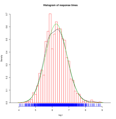
Figure 1: Transaction VA01, System 1: The figure shows the data points (logarithm of the response time in units of 1 ms, blue), a histogram (red), the density distribution (black) and the normal distribution with the same mean and variance. $\ln\,t=6$ corresponds to a response time $t\approx 400$ms, $\ln\,t=8$ corresponds to $t\approx 3000$ms. The basis are 324,000 data points.

Figure 1 shows results for VA01 in system 1. The distribution agrees quite well with a log-normal distribution, with a small deviation for $\tau\approx\tau_{m}$. The log-normal distribution has been calculated from the mean and variance of the actual data, no parameters have been adjusted. The data for VA02 and SESSION_MANAGER in system 1 and for SESSION_MANAGER in system 2 show a similar behaviour. Figs. 1 to 4 show an impressive agreement of the actual data with a log-normal distribution.

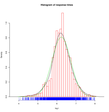
Figure 2: Transaction VA02, System 1: For details see Fig. 1. Basis: 419,000 data points.

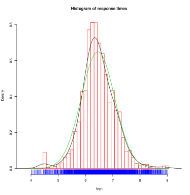
Figure 3: SESSION_MANAGER, System 1: For details see Fig. 1. The basis are 296,000 data points.

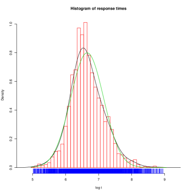
Figure 4: SESSION_MANAGER, System 2: For details see Fig. 1. Basis: 1,095,000 data points.

The agreement with the log-normal form does not only hold for the body of the response-time distributions, but, as far as we can judge from the data, also for the tails. The data show no hint of heavy tails.

III.3 Examples with a performance problem

It is interesting to study some examples where the response-time distribution differs from the log-normal form.

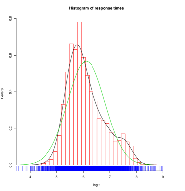
Figure 5: VA01, System 2: For details see Fig. 1. Basis are 143,000 data points.

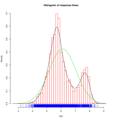
Figure 6: VA02, System 3: For details see Fig. 1. Basis: 281,000 data points.

The next two examples, VA01 in system 2 (Fig. 5) and VA02 in system 3 (Fig. 6) differ from a log-normal distribution. Esp. Fig. 6 shows a clear deviation from the log-normal distribution, the density curve has a bimodal form. This happens for instance if the transaction runs in two (or more) distinct situations with clearly different sets of parameters so that the distribution becomes a sum of two (or more) log-normal distributions. A similar, but less clear deviation can be observed in Fig. 5. For both cases one can show that the set of original data can be decomposed into two subsets, belonging to different parameter regimes. In both cases, the system was afflicted with a bottleneck during the period of measurement. The deviation from the log-normal form indicates a performance problem in the system.

A bimodal density curve as shown in the two examples is an indication of a performace problem. But the form of the density curve is not sufficient to find out, what kind of performance problem it is and how it can be cured. As mentioned above, we use the CCMS of the SAP system to collect many performance data, not only the response time. In a case like VA01 in system 2 (Fig. 5) one has to analyse these data: Does the problem occur generically, periodically or occasionally, does it occur for all users or for a special class of users, which contribution to the response time is responsible for the problem, etc. In the example VA01 in system 2 it turned out, that the problem occured for a special class of users, it could finally be traced back to a long time for sequential reads on a certain table of the database. After having solved the problem, the density curve had a log-normal form.

There are many different situations which yield a bimodal distribution curve. A simple example is a real bimodal situation, where the system runs on several, non-equivalent application servers. Another example is a system where, from time to time, periodically or casually, a bottleneck occurs. The actual reason for such a behaviour cannot be deduced from the response time data alone, but one needs a more complete set of performance data.

From a more general point of view the problem is that the response time for a given transaction as a function of its starting time may show correlations. Correlations occur because some of the external parameters (like CPU load or database load) vary in time, but on a time scale that is long compared to a typical response time. Correlations may be periodic in time because of a periodic usage of the system. Deviations from a log-normal distribution may occur due to such a periodic usage, as was the case in Fig. 6: This is a typical case for a periodic performance problem in a system. A similar form of the distribution can be observed if only a special class of users is affected by a performance problem, if the performance problem occurs due to a bottle neck in only one of several application servers, or in similar situations. In all of these cases the response time data are correlated.

Up to now we have shown results for transactions that are often used. But the overall result remains true even if a transaction is rarely used. As an example we finally show results for a proprietary transaction in system 1. The response-time distribution (Fig. 7) is again well described by a log-normal distribution; due to the smaller number of data points the fluctuations are larger. Furthermore the typical response time is longer, the median is $\tau_{m}\approx$3000 ms.

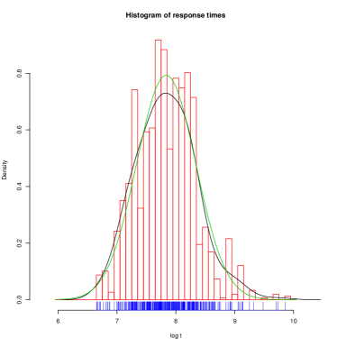
Figure 7: Transaction ZXXX, System 1: For details see Fig. 1. Basis: 1,722 data points.

III.4 General discussion of the log-normal form.

The above distributions of $\ln\tau$ are representative examples. Similar calculations can be done for many other transactions and for other systems. We made of performance measuremens in many SAP R/3 systems to identify and solve performance problems. For each case one can calculate how much the actual distribution of $\ln\tau$ differs from a normal distribution.

The difference of a distribution from the normal form can be described quantitatively by the higher cumulants $\kappa_{n}$, $n\geq 3$. Using the characteristic function

$$\phi(t)=\int dx\,p(x)\exp(itx)$$ (6)

of a distribution function $p(x)$ one defines the cumulants as the coefficients of the series

$$\ln\phi(t)=\sum_{n=0}^{\infty}\kappa_{n}\frac{(it)^{n}}{n!}$$ (7)

(see Abramowitz , number 26.1.12). The third and all higher cumulants vanish for a normal distribution, since the Fourier transform of a Gaussian is a Gaussian. Instead of the cumulants we calculate normalized cumulants $c_{n}=\kappa_{n}/\kappa_{2}^{n/2}$. $c_{3}$ is often called skewness, $c_{4}$ is the excess (or excess kurtosis) of the distribution. In Fig. 8 we show a $c_{3}$ vs. $c_{4}$ plot for measured distributions of $x=\ln\tau$ for various systems and transactions. For a log-normal distribution of $\tau$, i.e. a normal distribution of $x$, one would have $c_{3}=c_{4}=0$. For a majority of distributions the skewness is small ($|c_{3}|\lesssim 1)$ and the excess is small as well ($0\lesssim c_{4}\lesssim 1.5)$. On the other hand, the figure shows that larger deviations from the normal form occur. A negative value of $c_{4}$ often occurs in a situation with two or more maxima (e.g. in Fig 6). Furthermore, there is a clear tendency towards a positive skewness, which means that the statistical weight in the tail of the response-time distribution at long response times is even under-estimated by a log-normal distribution. In most of the cases shown in Fig. 8 a strong deviation from the log-normal form can be traced back to a performance problem in the system, where one of the heuristic rules mentioned above is violated.

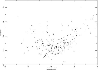
Figure 8: skewness vs. excess for 232 response-time distributions from 21 different SAP R/3 systems.

Although the data in Fig. 8 indicate that for a large subset the distribution function is close to a log-normal form, deviations occur. We may ask, whether a different form of the distribution function would give a better fit for these cases. A good candidate is certainly the generalized lambda distribution (GLD) discussed in Karian2000 ; Au-Yeung2004 . The GLD is a four parameter distribution. It has the ability to assume a wide variety of shapes. Whereas we used the first and the second moment to obtain the log-normal distribution shown in the previous examples, Au-Yeung et al. Au-Yeung2004 take the skewness $c_{3}$ and the excess $c_{4}$ to determine the two additional parameters. A point that has to be taken into account is that in Fig. 8 we plotted the skewness $c_{3}$ and the excess $c_{4}$ of the distribution of $\ln\tau$, whereas for the calculation of the GLD as described in Au-Yeung2004 we need the skewness $c_{3}$ and the excess $c_{4}$ of the distribution of $\tau$.

Let us briefly mention the main conclusion of our efforts using the GLD. As described in Au-Yeung2004 this distribution yields quite good results in situations with heavy tails, where the log-normal distribution is not applicable. But a heavy tail in the distribution would be considered as a performance problem and should not occur in a performant ERP system. On the other hand, the problem is that the GLD never describes a bimodal density curve. This means that the examples in section 3.3 cannot be described by a GLD. The same is true for most of the distribution functions represented by the points in Fig. 8. In most cases, where the probability distribution is not close to a log-normal form, the GLD fit of the probability distribution functions looks equally poor.

IV Discussion of the model

The simple model we introduced is a mean-field model. It is based on a set of assumptions expected to hold for an ideal system. The main ingredient is that $\ln\tau$ can be written as a sum of many contributions (4) and that correlations between the different contributions can be neglected.

The time for the central processes (reading, writing, processing data) yields the main contribution to the response time. Therefore one would naively expect that the corresponding time distributions are connected to the response-time distribution in a similar manner. A first idea could be to study the DB request time and the CPU time independently and to neglect any other contribution. But such an idea is misleading: Even if one could write the CPU time and the DB request time in a similar form as the response time in (4), the number of terms in the sum would be smaller and therefore the central limit theorem cannot be applied as well. To illustrate that such an idea is misleading, let us show the CPU time distribution and the DB request time distribution for the transaction VA01 in system 1. Whereas the response-time distribution in Fig. 1 is close to a log-normal form, the CPU time distribution (Fig. 9) and the DB request time distribution (Fig. 10) look quite different. The CPU time distribution shows clear deviations from a log-normal form. On the logarithmic time scale the distribution is skew. The DB request time distribution shows two maxima at 90 ms and at 1000 ms. The flanks are much steeper than for a log-normal distribution.

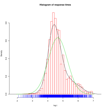
Figure 9: Transaction VA01, System 1: The figure shows the data points (logarithm of the response time in units of 1 ms, blue), a histogram (red), the density distribution (black) for the CPU time. The basis are 324,000 data points similar to Fig. 11.

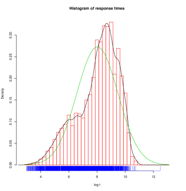
Figure 10: Transaction VA01, System 1: The figure shows the data points (logarithm of the response time in units of 1 ms, blue), a histogram (red), the density distribution (black) for the DB request times. The basis are 324,000 data points, similar to Fig. 11

Furthermore, the DB request time and the CPU time are correlated. The reason is that a transaction reads a certain amount of data from the database, performs operations on these data and eventually writes data to the database. Both, the CPU time (perfoming operations) and the DB request time (reading and writing data) depend on the same data.

Figure 11: Transaction VA01, System 1: The plot shows CPU time vs. DB request time.

The plot of the CPU time vs. DB request time for VA01 in system 1, Fig. 11, shows two cleary distinct regions, one where the CPU time is longer, the other where the DB request time is longer. Clearly the two maxima in Fig. 10 correspond to the two regions in Fig. 11.

In different systems or for different transactions the form of the distribution of the CPU time or the DB request time differ from the examples shown here. In most cases one learns more about the correlations in a suitable visulation of the data, as shown above, than using a sophisticated statistical method. There seems to be no universal form for the distribution of the CPU time or the DB request time. In contrast, our analysis indicates that the response-time distribution has a universal form, as long as we restrict ourselves to a “normal” situation without performance problems or other specialities.

Due to the correlations between the CPU time and the DB request time the joint distribution of these two quantities is not simply the product of the two distributions shown in Figs. 9 and 10. This means that the knowledge of these two distributions does not help if one wants to calculate the response-time distribution. In other words: In a complete theory correlations between CPU time and DB request time will play an essential role.

V Conclusions and Outlook

V.1 General remarks

The main result of this work is that the typical response-time distribution of transactions in an R/3 system has a log-normal form. This observation has several consequences for the interpretation of response time patterns in R/3 systems. The main point is that a log-normal distribution is skew and has a long tail for longer response times. As a consequence, the mean response time alone is not a good performance criterion. If the shape parameter $\sigma$ of the distribution, i.e., the variance of the normal distribution of $\ln\tau$, is large, long response times (twice or three times the mean response time) occur quite often. Without additional information about the distribution, e.g. the variance, one is not able to say whether or not the performance of the system is sufficiently good.

But the situation is even worse: Often one does not look at the response-time distribution of a single transaction, but at the response-time distribution of all dialog steps of a given group of transactions or reports, e.g., of all transactions and reports of a given module. If one observes for such a group of transactions a larger portion with longer response times, one often argues that this is due to batch-like reports running in dialog mode. This may of course be true, but another explanation may be the long tail of the log-normal distribution. This is a main difference: Whereas a user often knows that a certain report has a long run-time, he does not expect long response times for typical dialog transactions. Since the expectation of the user is different, the user satisfaction will be different as well.

In Sect. 2 we mentioned heuristic rules for the interpretation of response times. Although these rules help a lot in performance optimisation of R/3 systems, they have a severe drawback. This becomes clear when one looks at a distribution like the one shown in Fig. 6. The second, smaller peak may be a hint to a performance problem. The maximum of this peak occurs at $\tau\approx$2.5 s. But the weight of this peak is less than 10%, so that it will never be observed in averages. On the other hand, although there are correlations among the different contributions to the response time, the heuristic rules hold only for averages.

Deviations of the response-time distribution from a log-normal form may occur. A measure for the deviation is the skewness and the excess of the distribution of $\ln\tau$. Even if the mean response time is sufficiently short and if the variance is not too large, a large skewness or a large excess indicate that a large portion of dialog steps has long response times. Such deviations indicate a performance problem in the system. In other words: A plot like the one in Fig. 8 for a set of transactions in a given system can be used to identify problems in that system which cannot be seen regarding only averages and variances. Often, such performance problems are not even reported by users, esp. if it concerns an occasional user who considers the occasionally long response times as ’normal’.

V.2 Service level agreements

Another important aspect concerns service level agreements. It is clear that a simple agreement about the mean response time of all transactions is not suitable. On the other hand, simply due to practical restrictions, agreements on performance must be simple and it must be easy to verify them. One needs a possibility to measure the quantities that one uses in such an agreement.

We already mentioned that most ERP system contain builtin tools to measure response times. Builtin reports yield only averages for the response times of transactions, but it is a simple task to write a small program that uses the builtin functionality to calculate other statistical information as well.

From the above discussion one would suggest the following rules:

• Agreements on specific transactions are better than global statements on averages over a large group of transactions, since the behaviour of different transactions is different and bottlenecks affect different transactions in a different way. But if the number of different transactions is too large, one should restrict agreements to a small set of transactions, e.g., the ten most important transactions in a system.

• In addition to a mean response time, one needs a second parameter to control the variance of the distribution. But this is only suitable in a situation without a bottleneck, where the form of the response-time distribution is close to log-normal. Generically, an agreement that states that a certain portion of all dialog steps for certain transactions should have a sufficiently small response time (e.g. “80% of all dialog steps of a given class of transactions should have a response time less than one second”) is much better than an agreement on averages, since it allows some control on the tail of the response-time distribution.

Which class of transactions is actually chosen and what quantile is suitable depends on the actual system for which a service level agreement is needed.

V.3 Future work

There are three main directions for future work on peformance of ERP systems:

1. A much more detailed analysis of the data is needed to better understand correlations between the different contributions to the response time.

2. A microscopic model is needed to better understand the deviations from log-normal form. Such a model should also be able to include and explain correlations between the different parameters in the system.

3. There are many reasons why the complexity of the ERP system landscape in large enterprises is growing: more business processes are supported by such systems, due to legal reasons additional functionality is needed, etc. Therefore new types of such systems with special functionality are needed. Examples are business warehouse systems, customer relationship management systems, supply chain management systems. It is not clear whether or how the results presented in this paper can be generalized to such new systems.

The general goal behind these steps is to obtain a detailed understanding of the response time statistics of ERP systems.

References

- (1) K. S. Trivedi, S. Ramani, and R. Fricks: Recent Advances in Modeling Response-Time Distributions in Real-Time Systems. PROCEEDINGS OF THE IEEE 8, 1023-1037 (2003).
- (2) S.W.M. Au-Yeung, N.J. Dingle, and W.J. Knottenbelt: Efficient Approximation of Response Time Densities and Quantiles in Stochastic Models. Proc. 4th ACM Workshop on Software and Performance (WOSP 2004), Redwood City, California, USA, January 2004, pp. 151-155.
- (3) T. Schneider: SAP-Performanceoptimierung. SAP-Press, Galileo Press, Bonn 20022.
- (4) V. Paxson: Empirically-Derived Analytic Models of Wide-Area TCP Connections. IEEE/ACM Transactions on Networking 2, No. 4 (1994)
- (5) Mark E. Crovella and Azer Bestavros: Explaining World Wide Web Traffic Self-Similarity. TR-95-015, Boston University Computer Science Department, Revised, October 12, 1995.
- (6) R. V. Sole and S. Valverde: Information transfer and phase transitions in a model of Internet Traffic. Physica A 289, 595-605 (2001)
- (7) W. Willinger, V. Paxson, and M.S. Taqqu: Self-similarity and Heavy Tails: Structural Modeling of Network Traffic. In A Practical Guide to Heavy Tails: Statistical Techniques and Applications, Adler, R., Feldman, R., and Taqqu, M.S., editors, Birkhauser, 1998.
- (8) M. Arlitt, D. Krishnamurthy, and J. Rolia: Characterizing the Scalability of a Large Web-based Shopping System”, ACM Transactions on Internet Technology 1, 44-69 (2001).
- (9) H. Risken: The Fokker-Planck Equation. Springer, Berlin, Heidelberg, New York 19892.
- (10) M. Abramowitz, I.A. Stegun: Handbook of Mathematical Functions. Dover Publications, New York 19709.
- (11) Z. Karian and E. Dudewicz. Fitting Statistical Distributions: The Generalized Lambda Distribution and Generalized Bootstrap Methods. CRC Press, Boca Raton, 2000.