New Visualization of Surfaces in Parallel Coordinates
– Eliminating Ambiguity and Some “Over-Plotting”

Abstract

$\cal{A}$ point $P\in\mathbb{R}^{n}$ is represented in Parallel Coordinates by a polygonal line $\bar{P}$ (see [Ins99] for a recent survey). Earlier [Ins85], a surface $\sigma$ was represented as the envelope of the polygonal lines representing it’s points. This is ambiguous in the sense that different surfaces can provide the same envelopes. Here the ambiguity is eliminated by considering the surface $\sigma$ as the envelope of it’s tangent planes and in turn, representing each of these planes by $n$-$1$ points [Ins99]. This, with some future extension, can yield a new and unambiguous representation, $\bar{\sigma}$, of the surface consisting of $n$-$1$ planar regions whose properties correspond lead to the recognition of the surfaces’ properties i.e. developable, ruled etc. [Hun92]) and classification criteria.

It is further shown that the image (i.e. representation) of an algebraic surface of degree $2$ in $\mathbb{R}^{n}$ is a region whose boundary is also an algebraic curve of degree $2$. This includes some non-convex surfaces which with the previous ambiguous representation could not be treated. An efficient construction algorithm for the representation of the quadratic surfaces (given either by explicit or implicit equation) is provided. The results obtained are suitable for applications, to be presented in a future paper, and in particular for the approximation of complex surfaces based on their planar images. An additional benefit is the elimination of the “over-plotting” problem i.e. the “bunching” of polygonal lines which often obscure part of the parallel-coordinate display.

keywords: Scientific Visualization and HMI.

AMS : 76M27

1 INTRODUCTION

Our purpose here is expository, sparing the reader from most of the mathematical tribulations and, focusing on the more intuitive aspects of the representational results. After a short review of the fundamentals, the essentials of the mathematical development are given together with some detailed examples to clarify the nuances and satisfy the more mathematically inclined.

In parallel coordinates (abbr. $\|$-coords), a point in $\mathbb{R}^{2}$ is represented by a line and a line is represented by a point yielding a fundamental $point\leftrightarrow line$ duality. There follows the representation of $p$-flats (planes of dimension $2\leq p\leq n-1$) in $\mathbb{R}^{n}$ in terms of indexed points [Ins85]. Naturally, for non-linear objects the representation is more complex, especially if they are also non-convex. The points of a curve in $\mathbb{R}^{2}$ can be mapped directly into a family of lines whose envelope defines a curve (“line-curve”). Actually this is awkward and also clutters the display. Instead we map the tangents of the original curve into points to obtain the “point-curve”, sometimes called “dual-curve”, image directly as shown in Fig. 1. In short, this approach provides a convenient point-to-point mapping [Ins99].

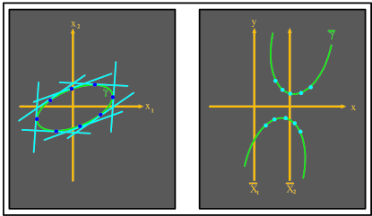
Figure 1: Point-curve mapped into point-curve, result of considering the point-curve as the envelope of it’s tangents.

Applying these considerations it was proved that the image of an algebraic curve of degree $n$ is also algebraic of degree at most $n(n-1)$ in the absence of singular points [Izh01]. This theorem is a generalization of the known result that conics are mapped into conics [Dim84] in six different ways.

Perhaps we are “pushing our luck”, our intent is to apply next the point-to-point mapping in the representation of surfaces considered as the envelope of their tangent planes; with the resulting image being constructed from the representation of tangent planes [Ins99]. As has already been pointed out, planes can be represented in $\|$-coords by indexed points. The collection of these planar points, grouped for each index, is the representation of the surface.

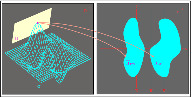
Figure 2: For a hyper-surface, it’s representation’s boundary curves are determined

from the images of curves contained in hyper-surface.

In the past [Ins85], surfaces were represented in $\|$-coords by the envelope of the polygonal lines representing the surfaces’ points. By itself this is ambiguous. For example the image of a sphere in $n$-dimensions is the same as the image of the surface obtained by the intersection of $n$ cylinders properly aligned having the same radius. In applications this was ameliorated by accessing the correct equation of the surface when needed. Not only is the ambiguity completely removed with the new representation, but also non-convex surfaces can be nicely treated something that was not possible previously.

Hung [Hun92] first applied this notion and found that regions representing developable surfaces consists only of the boundary curves (i.e. there are no interior points), and also that ruled surfaces can be recognized from characteristic properties of their corresponding regions. Encouraged by these initial results the analysis is extended to more general surfaces yielding useful criteria in the approximation of surfaces by simpler ones; but we are getting ahead of ourselves.

At first we lay the foundations, then derive the representation of quadratic algebraic surfaces and further generalize to higher dimension as well as more complex hyper-surfaces. As a result an efficient algorithm for constructing the representation of the quadratic surfaces (given either by explicit or implicit equation), and a proof that the image of an algebraic surface of degree $2$ in $\mathbb{R}^{n}$ is also an algebraic curve and of degree $2$ are obtained.

2 GENERAL REPRESENTATION OF HYPER-SURFACE

$\cal{I}$n general, the method employed below applies to the class of smooth hyper-surfaces in $\mathbb{R}^{n}$ having a unique tangent hyper-plane at each point. Equivalently, each such hyper-surface is the envelope of it’s tangent hyper-planes. This is our point of departure, for it enables us to represent each tangent hyper-plane in $\|$-coords by $n-1$ indexed points [Ins99]. The hyper-surface’s representation consists of the $n-1$ points sets, one for each index [Hun92]. For the present we restrict our attention to algebraic hyper-surfaces and in particular those defined by quadratic polynomials. To simplify matters, most of the analysis is done in 3-dimensional space but in a way which points to the generalization for $\mathbb{R}^{n}$.

2.1 Hyper-Planes Representation

An $n$-dimensional hyper-plane $\pi$ in $\mathbb{R}^{n}$

$$\pi:\sum_{i=1}^{n}c_{i}x_{i}=c_{0},$$ (1)

is represented by the $n-1$ indexed points [Ins99]. For our purposes only the first

$$\bar{\pi}_{1\dots n}=(\sum_{i=1}^{n}(i-1)c_{i},c_{0},\sum_{i=1}^{n}c_{i}).$$ (2)

needs to be studied. The remaining $n-2$ points have similar form differing only in the factor $(i-1)$ of the $c_{i}$. An important property is that the horizontal distance between the $i$-adjacent (in the indexing) points is the equal to the coefficient $c_{i}$; from which the sequence of indexed points can be generated from the coefficients or vice-versa.

2.2 Hyper-Surfaces Representation

Moving on to the representation of non-linear hyper-surfaces in $\mathbb{R}^{n}$ from their tangent hyper-planes. Let $\sigma$ be a smooth $n$-dimensional hyper-surface generated by the differentiable function $F(x_{1},\dots,x_{n})=0$, and an arbitrary point $(x^{0}_{1},\dots,x^{0}_{n})\in\sigma$. Then the hyper-surface’s tangent hyper-plane at this point is given by :

$$\sum_{i=1}^{n}(x_{i}-x^{0}_{i})\frac{\partial{F}}{\partial{x_{i}}}(x^{0}_{1},\dots,x^{0}_{n})=0.$$

Taking the $x^{0}_{i}$ as parameters, the coefficients of the tangent hyper-planes can written as a function of points which satisfy the hyper-surface’s equation. Namely, the family of tangent hyper-planes of $\sigma$ is represented in homogenous coordinates, by a collection of sets $\bar{\sigma}$ (see Fig. 2), containing the indexed points representing each member (i.e. hyper-plane) of the family. Each of the $n-1$ indexed set, $\bar{\sigma}_{j\dots n1^{\prime}\dots(j-1)^{\prime}}$, consists of the points with the same index.

In the remainder the analysis is confined to the first indexed set $\bar{\sigma}_{1\dots n}$ using a shorter notation $\bar{\sigma}$ defined as,

$$\bar{\sigma}=\left\{\left(P(\bar{x}),\;S(\bar{x}),\;Q(\bar{x})\right)\;|\;\bar{x}\in\sigma)\right\},$$ (3)

where for $\bar{\sigma}_{1\dots n}$ and the tuple $\bar{x}=(x_{1},\dots,x_{n})$ :

$${}P(\bar{x}) = \sum_{i=1}^{n}(i-1)\frac{\partial{F}}{\partial{x_{i}}}$$

$$S(\bar{x}) = \sum_{i=1}^{n}x_{i}\frac{\partial{F}}{\partial{x_{i}}}$$ (4)

$$Q(\bar{x}) = \sum_{i=1}^{n}\frac{\partial{F}}{\partial{x_{i}}}.$$

In general, the representation in $\|$-coords is constructed via the rational transformations

$$x=\frac{P(\bar{x})}{Q(\bar{x})}\;\;\;,\;\;\;y=\frac{S(\bar{x})}{Q(\bar{x})}.$$ (5)

The representation of all these hyper-planes transform an $n$-dimensional hyper-surface into subsets of $\mathbb{P}^{2}$; regions which are distinguished from each other by their indices. The algorithm which constructs and describes these regions is presented next.

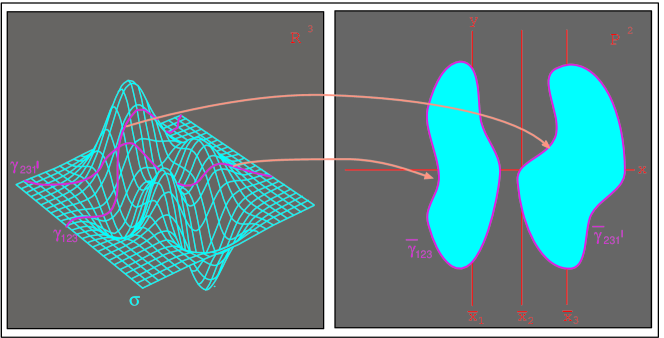
Figure 3: The boundary of each region is an image of a curve embedded in surface.

3 REPRESENTATION OF QUADRAT- IC   HYPER-SURFACE

$\cal{A}$t first we treat the class of algebraic surfaces in ${\mathbb{R}}^{3}$ described by quadratic polynomials. Mercifully, the corresponding system of transformations (2.2) can be linearized. The next step is to determine the boundary of the regions representing the surface. Without getting into details, the existence of the boundary can be assured by selecting an appropriate spacing of axes in the system of the $\|$-coords, which eventually reflect by changing the constant multipliers of the first equation in (2.2).

3.1 Definition of the Regions’ Boundary

Let $\sigma$ be a quadratic surface whose representation is the region $\bar{\sigma}$. The boundary points are those whose every neighborhood contains both interior and exterior points. For this case both the transformation (2.2) and the surface, are defined by polynomials and hence are differentiable. The basic properties including continuity are therefore preserved under the transformation.

Geometrically we rely on the differentiability in finding those points $\bar{p}\in\bar{\sigma}$ so that we can “move” from $\bar{p}$ in any direction and still remain in region; these are interior points of $\bar{\sigma}$. Clearly the boundary points are easily found as the complement of the interior of $\bar{\sigma}$. The condition for determining whether a point is interior or not is given by theorem of implicit function [Mar85]. Equivalently, a point $\bar{a}\in\bar{\sigma}$ is interior point if and only if the Jacobian, $J(F)|_{\bar{a}}$, at this point is different from zero. Conversely, a point $\bar{b}\in\bar{\sigma}$ for which this is not true is necessarily a boundary point; namely, a point $\bar{b}\in\bar{\sigma}$ s.t. $J(F)|_{\bar{b}}=0$. In essence the theorem tells us that $\bar{\sigma}$ is closed set and the complement of its interior is the sought after boundary.

Generalizing the above for $\mathbb{R}^{n}$ we get the mapping $(x_{1},\dots,x_{n})\rightarrow(\eta,\xi,\psi)$ into the projective space, were $x=\frac{\eta}{\psi}$ and $y=\frac{\xi}{\psi}$. Restating the condition in terms of differential products using homogeneous coordinates with the variables $\eta$, $\xi$ and $\psi$ yields,

$$(\eta d\xi d\psi-\xi d\eta d\psi+\psi d\eta d\xi)dF=0.$$ (6)

This form is more convenient for handling hyper-surfaces embedded in $\mathbb{R}^{n}$ where $n>3$, for $n=3$ eq. (6) can be written equivalently in term of Jacobian as,

$$J(F)\psi^{3}=Det\left[\matrix{\frac{\partial{F}}{\partial{x_{1}}}&\frac{\partial{F}}{\partial{x_{2}}}&\frac{\partial{F}}{\partial{x_{3}}}\cr\frac{\partial{(\eta/\psi)}}{\partial{x_{1}}}&\frac{\partial{(\eta/\psi)}}{\partial{x_{2}}}&\frac{\partial{(\eta/\psi)}}{\partial{x_{3}}}\cr\frac{\partial{(\xi/\psi)}}{\partial{x_{1}}}&\frac{\partial{(\xi/\psi)}}{\partial{x_{2}}}&\frac{\partial{(\xi/\psi)}}{\partial{x_{3}}}\cr}\right]\psi^{3}.$$ (7)

Substituting $\eta$, $\xi$ and $\psi$ in terms of the $x_{i}$’s yields an equation which defines an algebraic surface, $\sigma^{\prime}$, in $\mathbb{R}^{3}$. Geometrically, the boundary $\bar{\gamma}$ consist of points which represent tangent planes touching at points of $\sigma$ on the intersection $\sigma^{\prime}\cap\sigma$. Hence, $\bar{\gamma}$ is the image of the algebraic curve $\sigma^{\prime}\cap\sigma=\gamma$ (see Fig. 3).

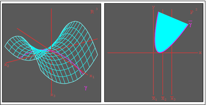
Figure 4: Saddle $\sigma$: $z=-(x/2)^{2}+(y/2)^{2}\;\;\rightarrow\;\;\bar{\gamma}:16-16x-4y+y^{2}-4xy+4x^{2}=0$.

Combining the criterion, eq. (7), for the boundary with the equation of the surface (embedded in 3-dimensional space) and the transformation equations (in homogenous coordinates) yields :

$$\begin{array}[]{lll}F(x_{1},x_{2},x_{3})&=0,\\ \eta Q(x_{1},x_{2},x_{3})-\psi P(x_{1},x_{2},x_{3})&=0,\\ \xi Q(x_{1},x_{2},x_{3})-\psi S(x_{1},x_{2},x_{3})&=0,\\ J(F(x_{1},x_{2},x_{3}))\psi^{3}&=0.\end{array}$$ (8)

Solving for $\eta$, $\xi$ and $\psi$ yields the equation of the boundary. Note that if $F$ is a polynomial of degree $2$, then the degree of $J(F)\psi^{3}$ is $\leq 2$ in terms of all variables, while it is linear in terms of $x_{1}$, $x_{2}$ and $x_{3}$.

Thus far we have constructed a system of four equations (8) in six variables which define a mapping from the $\mathbb{R}^{3}$ into the projective plane $\mathbb{P}^{2}$. Our aim, is to determine the specific equation of the region’s boundary explicitly. This involves solving this system of equations in terms of $\eta$, $\xi$ and $\psi$ by eliminating the variables $x_{1}$, $x_{2}$ and $x_{3}$.

The equation’s structure turns out to be very advantageous. Since the last three equations are linear, the elimination can be done by isolating a variable (finding an explicit expression in term of the other variables), and substituting in the remaining linear equations. When all is said and done, each of the variables $x_{1}$, $x_{2}$ and $x_{3}$ can be expressed as a rational equation in $\eta$, $\xi$ and $\psi$. Upon substitution of these expressions into $F$ the boundary’s equation in homogeneous coordinates is obtained. It follows that the boundary $\bar{\gamma}$ is a quadratic curve.

3.2 Algorithm

The algorithm’s input is an equation of algebraic surface $\sigma:F(x_{1},x_{2},x_{2})=0$ of degree two and the output is the polynomial which describes the boundary of the surface’s image in $\|$-coords. It is noteworthy that the algorithm applies to implicit or explicit polynomials with or without singular points. The formal description is followed by examples which clarify the various stages and their nuances.

For a given polynomial equation $F(x_{1},x_{2},x_{3})=0$ of degree 2 and a spacing of axes $S_{1\dots n}$:

• Let :

  $\qquad\eta=\sum_{i=1}^{3}(i-1)\frac{\partial{F}}{\partial{x_{i}}}\;,$

  $\qquad\xi=\sum_{i=1}^{3}x_{i}\frac{\partial{F}}{\partial{x_{i}}}-2F\;,$

  $\qquad\psi=\sum_{i=1}^{3}\frac{\partial{F}}{\partial{x_{i}}}.$

• Write the three linear equations:

  $a)$ $\qquad\psi\sum_{i=1}^{3}(i-1)\frac{\partial{F}}{\partial{x_{i}}}-\eta\sum_{i=1}^{3}\frac{\partial{F}}{\partial{x_{i}}}=0,$

  $b)$ $\qquad\psi(\sum_{i=1}^{3}x_{i}\frac{\partial{F}}{\partial{x_{i}}}-2F)-\xi\sum_{i=1}^{3}\frac{\partial{F}}{\partial{x_{i}}}=0,$

  $c)$ $\qquad J(F)\psi^{3}=0.$

• Using substitution write

  $\qquad x_{i}=f_{i}(\eta,\xi,\psi)\;$,     for $i=1,2,3$.

• Substitute

  $\qquad F(f_{1}(\eta,\xi,\psi),f_{2}(\eta,\xi,\psi),f_{3}(\eta,\xi,\psi))=0.$

• Retain the equation’s numerator.

• The output is obtained by substitution:

  $\qquad\eta\leftarrow x\;\;,\;\;\xi\leftarrow y\;\;,\;\;\psi\leftarrow 1.$

All this falls into place with the following examples.

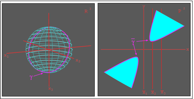
Figure 5: Sphere $\sigma$: $x^{2}+y^{2}+z^{2}=2\;\;\rightarrow\;\;\bar{\gamma}:x^{2}-4xy+y^{2}+1=0$.

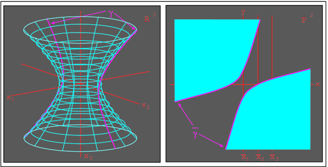
Figure 6: Hyperboloid of one sheet $\sigma$ : $x^{2}+y^{2}-z^{2}=1\;\;\rightarrow\;\;\bar{\gamma}:x^{2}-4xy+y^{2}-1=0$.

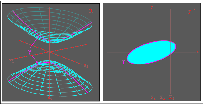
Figure 7: Hyperboloid of two sheets $\sigma$: $x^{2}-4y^{2}+2z^{2}=-2\;\;\rightarrow\;\;\bar{\gamma}:x^{2}-2xy+4y^{2}-1=0$.

4 EXAMPLE OF QUADRATIC SURFACE AND THEIR TRANSFORMS

$\cal{I}$n the first example is quite detailed to accommodate the readers wishing to follow the application of the algorithm in depth. Let $\sigma$ be $3$-dimensional saddle (see Fig 4) generated by the polynomial equation,

$F(\bar{x})=\left(\frac{x_{1}}{2}\right)^{2}-\left(\frac{x_{2}}{2}\right)^{2}+x_{3}=x_{1}^{2}-x_{2}^{2}+4x_{3}=0$, where $\bar{x}=(x_{1},x_{2},x_{3})$, and $S_{1\dots n}$ the standard spacing of axes.

step 1

Let :

$\begin{array}[]{llll}P(\bar{x})=&\sum_{i=1}^{3}(i-1)\frac{\partial{F}}{\partial{x_{i}}}&=&-2x_{2}+8,\\ S(\bar{x})=&\sum_{i=1}^{3}x_{i}\frac{\partial{F}}{\partial{x_{i}}}-2F&=&-4x_{3},\\ Q(\bar{x})=&\sum_{i=1}^{3}\frac{\partial{F}}{\partial{x_{i}}}&=&2x_{1}-2x_{2}+4.\end{array}$

step 2

Write the three linear equations:

$a)$ $\eta Q(\bar{x})-\psi P(\bar{x})=$

$\qquad\qquad 2(\eta x_{1}+(\psi-\eta)x_{2}+2\eta-4\psi)=0$,

$b)$ $\xi Q(\bar{x})-\psi S(\bar{x})=$

$\qquad\qquad 2(\xi x_{1}-\xi x_{2}+2\psi x_{3}+2\xi)=0$,

$c)$ $J(F(\bar{x}))\psi^{3}=(x_{1}(\psi-\eta)+x_{2}\eta-\xi)$.

Notice: substitution of $\eta$, $\xi$ and $\psi$ in terms of $x_{1}$, $x_{2}$ and $x_{3}$ yields a surface in $\mathbb{R}^{3}$,

$\qquad\sigma^{\prime}:32(-x_{2}^{2}+4x_{2}+x_{1}^{2}+2x_{3}-2x_{1})=0$.

Hence $\gamma=\sigma^{\prime}\cap\sigma$,

$\qquad\gamma:\;\;\left\{\begin{array}[]{llll}x_{1}^{2}-x_{2}^{2}+4x_{3}&=0\\ -x_{2}^{2}+4x_{2}+x_{1}^{2}+2x_{3}-2x_{1}&=0\end{array}\right.$.

step 3

Using simple substitution write

$b)$ $\Rightarrow\;x_{3}=-\frac{\xi(x_{1}-x_{2}+2)}{2\psi}$,

$c)$ $\Rightarrow x_{2}=-\frac{(\psi-\eta)x_{1}-\xi}{\eta}$.

Then using equation $a)$ we get,

$\qquad x_{1}=-\frac{-2\eta^{2}+\eta\xi-\psi\xi+4\psi\eta}{\psi\left(\psi-2\eta\right)},$

$\qquad x_{2}=\frac{2\eta^{2}-\eta\xi-6\psi\eta+4\psi^{2}}{\psi\left(\psi-2\eta\right)},$

$\qquad x_{3}=\frac{\xi(-\xi+2\eta+2\psi)}{2\psi(\psi-2\eta)}$.

step 4

Substitute in $F$,

$x_{1}^{2}-x_{2}^{2}+4x_{3}=$

$\qquad-\frac{16\psi^{2}-16\psi\eta-4\psi\xi+\xi^{2}-4\eta\xi+4\eta^{2}}{\psi\left(\psi-2\eta\right)}=0$.

step 5

Retain the equation’s numerator,

$16\psi^{2}-16\psi\eta-4\psi\xi+\xi^{2}-4\eta\xi+4\eta^{2}=0$.

step 6

Finally, the output is obtained by substitution,

$\eta\leftarrow x\;\;,\;\;\xi\leftarrow y\;\;,\;\;\psi\leftarrow 1$:

$\bar{\gamma}:\;\;16-16x-4y+y^{2}-4xy+4x^{2}=0.$

The surface and its image including the boundary curve are shown in Fig 4. The representation of other quadratic surfaces is illustrated in figures 5, 6 and 7.

5 CONCLUSION

$\cal{T}$he new representation

• is constructive,

• enables the representation of non-convex objects,

• maps algebraic surfaces to regions having algebraic curves as boundaries,

An important “fringe benefit” is the avoidance of the “over-plotting” problem in $\|$-coords where polygonal lines obscure portions of the display.

References

- [Cox97] Cox, D., Little, J., and O’Shea, D. 1997. Ideals, Varieties, and Algorithms, second ed. ed. Springer, New York.
- [Dim84] Dimsdale, B., 1984. Conic transformations and projectivities. IBM Los Angeles Scientific Center. Rep. G320-2753.
- [Har92] Harris, J. 1992. Algebraic Geometry, vol. A rst course. Springer, NY.
- [Hun92] Hung, C., and Inselberg, A., 1992. Parallel coordinates representation of smooth hypersurfaces. IBM Palo Alto Scientific Center. Tech Rep. G320-3575.
- [Ins85] Inselberg, A. 1985. The plane with parallel coordinates. The Visual Computer 1, 2, 69–92.
- [Ins99] Inselberg, A. 1999. Don’t panic … do it in parallel! Computational Statistics 14, 53–77.
- [Izh01] Izhakian, Z. 2001. An Algorithm For Computing A Polynomial’s Dual Curve In Parallel Coordinates. M.sc thesis, University of Tel Aviv.
- [Mar85] Marsden, J., and Weinstein, A. 1985. Calculus. Springer-Verlag, New York.