Genetic Algorithms and Quantum Computation

Abstract

Recently, researchers have applied genetic algorithms (GAs) to address some problems in quantum computation. Also, there has been some works in the designing of genetic algorithms based on quantum theoretical concepts and techniques. The so called Quantum Evolutionary Programming has two major sub-areas: Quantum Inspired Genetic Algorithms (QIGAs) and Quantum Genetic Algorithms (QGAs). The former adopts qubit chromosomes as representations and employs quantum gates for the search of the best solution. The later tries to solve a key question in this field: what GAs will look like as an implementation on quantum hardware? As we shall see, there is not a complete answer for this question. An important point for QGAs is to build a quantum algorithm that takes advantage of both the GA and quantum computing parallelism as well as true randomness provided by quantum computers. In the first part of this paper we present a survey of the main works in GAs plus quantum computing including also our works in this area. Henceforth, we review some basic concepts in quantum computation and GAs and emphasize their inherent parallelism. Next, we review the application of GAs for learning quantum operators and circuit design. Then, quantum evolutionary programming is considered. Finally, we present our current research in this field and some perspectives.
Keywords: Genetic Algorithms, Quantum Computing, Evolutionary Strategies.

1 Introduction

Our aim in this paper is two-fold. Firstly, we review the main works in the application of Genetic Algorithms (GAs) for quantum computing as well as in the Quantum Evolutionary Programming. Secondly, based on this review, we offer new perspectives in the area which are part of our current research in this field.

In the last two decades we observed a growing interest in Quantum Computation and Quantum Information due to the possibility to efficiently solve hard problems for conventional computer science paradigms. Quantum computation and quantum information encompass processing and transmission of data stored in quantum states (see [20] and references therein). In these fields, the computation is viewed as effected by the evolution of a physical system, which is governed by unitary operators, according to the Laws of Quantum Mechanics [19]. The basic unity information is the qubit, the counterpart in quantum computing to the classical $0-1$ bit. Quantum Computation and Quantum Information explore quantum effects, like quantum parallelism, superposition of states and entanglement in order to achieve a computational theory more efficient than the classical ones. This has been demonstrated through quantum factoring and Grover’s algorithm for database search [14].

On the other hand, Genetic Algorithms (GAs) is a rapidly expanding area of current research. They were invented by John Holland in the 1960s [13]. Simply stated, GAs are stochastic search algorithms based on the mechanics of natural selection and natural genetics [9, 16, 15]. They have attracted people from a wide variety of disciplines, mainly due to its capabilities for searching large and non-linear spaces where traditional methods are not efficient [9].

From this scenario, emerge the application of genetic algorithms for quantum computation as well as evolutionary programming based on quantum theoretical concepts and techniques. Despite of the fact that there are few works in these subjects yet, it is an exciting area of research in the field of evolutionary computation.

When applying GAs, people are attracted by their capabilities for searching a solution in non-usual spaces. That is way people investigate the application of GAs for learning quantum operators [6, 8] and in the designing of quantum circuits [31, 29, 23].

Those works rely on the fundamental result for quantum computing that all the computation can be expanded in a circuit which nodes are the universal gates [19]. These gates offer an expansion of an unitary operator $U$ that evolves the system in order to perform some computation [19, 14]. Thus, we are naturally in the face of two classes of problems: (1) Given a set of functional points $S=\left\{\left(x,y\right)\right\}$ find the operator $U$ such that $y=U\cdot x$; (2) Given a problem, find a quantum circuit that solves it. The former was formulated in the context of GAs for learning algorithms [6, 8] while the latter through evolutionary strategies [31, 29, 23].

In [6] we proposed a method based on genetic algorithms to learn linear operators. The method was applied for learning quantum (unitary) operators. It was demonstrated that it overcomes the limitations of the work proposed by Dan Ventura [28], which resembles basic methods in neural networks.

For the second class of problems, we found three schemes outlined by Spector [27], based on the traditional tree-based genetic programming [15], stackless and stack-based linear genome. Moreover, in another scheme proposed by Williams and Gray [29], an unitary matrix for a known quantum circuit is used to find possible alternative circuits.

More close to our actual research are the works by Rubinstein [23] and Yabuki [31]. The production of entangled states and the quantum teleportation were the target problems in these works. In [23] each gate is encoded through a structure (gate structures) and a quantum circuit is represented as a list of such structures. Then, genetic operators (crossover and mutation) are applied in order to evolve a randomly chosen initial population of circuits. A special fitness function was also proposed and the scheme applied to find circuits for entangled states production. Yabuki and Iba follow a similar philosophy in [31] but changing the circuit representation. The quantum teleportation was the focused problem. In this case, authors performed a circuit optimization; that is, they start with a seed circuit that had eleven gates and obtained another one, with just eight gates, but that performs the same computation. That is a variant of the second class of problems.

By 1996, Narayan and Moore [17] introduced a novel evolutionary computing method where concepts and principles of quantum computing are used to inspire evolutionary strategies. It was the first attempt towards quantum evolutionary programming. The basic approach is inspired on the multiple universes view of quantum theory: each universe contains its own population of chromosomes. The populations in each universe obey identical classical rules and evolve in parallel. However, just after classical crossover within each universe, the universes can interfere with one another which induces some kind of crossover involving the chromosomes.

Narayan and Moore’s method depends on non-standard interpretations of Quantum Mechanics. The lack of a more formal analysis of the physical concepts used brings difficulties to make the correlation between the physics and the genetic algorithm itself. Consequently it does not offer clues of the advantages of a quantum implementation for GAs within the current implementations of quantum computers [20]. Thus, we are not going to consider it in the following sections.

In [11] we found another Quantum Inspired Genetic Algorithm (QIGA) which relies on usual methods of Quantum Mechanics. It is characterized by principles of quantum computing, including concepts of qubits and superposition of states, as well as quantum operators to improve convergence. An important consequence of this work is to emphasize that the application of quantum computing concepts to evolutionary programming is a promising field.

Rylander et al. [25] kept this idea and sketched out a Quantum Genetic Algorithm (QGA) which takes advantage of both the quantum computing and GAs parallelism. Despite of the lack of a mathematical explanation about the physical realization of the algorithm, we will show that its philosophy is close to an implementation in current experimental architectures for quantum computers [20]. The key idea is to explore the quantum effects of superposition and entanglement to create a physical state that store individuals and their fitness. When measure the fitness, the system collapses to a superposition of states that have that observed fitness. Starting from this idea, we propose in section 5 a QGA which can take advantage of both quantum computing and GAs paradigms. We present its physical foundations and discuss its advantages over classical GAs.

This paper is organized as follows. Firstly, we give the necessary background in quantum computation (section 2.1) and genetic algorithms (section 2.2). Then, the review sections start. We begin with the GAs applications in quantum computation. So, in section 3.1 we describe our work on GAs for learning quantum operators. Section 3.2 presents the works on GAs for circuit design. Following, in section 4, we offer the review of quantum evolutionary approaches. The QIGA proposed in [11] is presented on section 4.1. We end the review by presenting on section 4.2 the QGA proposed in [25]. In section 5 we discuss the considered methods and describe some issues. In particular, we propose a physical model for the QGA. Finally, we present the conclusions on section 6.

2 Background in Quantum Computation and GAs

2.1 Quantum Computation

In practice, the most useful model for quantum computation is the Quantum Circuit one [19, 21]. The basic information unit in this model is a qubit [19], which can be considered a superposition of two independent states $\mid 0\rangle$ and $\mid 1\rangle$ , denoted by $\mid\psi\rangle=\alpha_{0}\mid 0\rangle+\alpha_{1}\mid 1\rangle$, where $\alpha_{0},\alpha_{1}$ are complex numbers such that $\left|\alpha_{0}\right|^{2}+\left|\alpha_{1}\right|^{2}=1$. They are interpreted as probability amplitudes of the states $\mid 0\rangle$ and $\mid 1\rangle.$

A composed system with $n$ qubits is described using $N=2^{n}$ independent states obtained through the tensor product of the Hilbert Space associated with each qubit. Its physical realization is called a quantum register. The resulting space has a natural basis that can be denoted by:

$$\left\{\mid i_{0}i_{1}...i_{n-1}\rangle;\quad i_{j}\in\left\{0,1\right\},\quad j=0,1,...,n-1\right\},$$ (1)

where we are using the Dirac notation for vectors in Hilbert spaces.

This set can be indexed by $\mid i\rangle;\quad i=0,1,...,N-1.$ Following the Quantum Mechanics Postulates [19], the state $\mid\psi\rangle,$ of a system, in any time $t,$ can be expanded as a superposition of the basis states:

$$\mid\psi\rangle=\sum_{i=0}^{N-1}\alpha_{i}\mid i\rangle;\quad\sum_{i=0}^{N-1}\left|\alpha_{i}\right|^{2}=1.$$ (2)

Entanglement is another important concept for quantum computation with no classical counterpart. To understand it, a simple example is worthwhile.

Let us suppose that we have a composed system with two qubits. According to the above explanation, the resulting Hilbert Space has $N=2^{2}$ independent states.

Let the Hilbert Space associated with the first qubit (indexed by $1$) denoted by $H_{1}$ and the Hilbert Space associated with the second qubit (indexed by $2$) denoted by $H_{2}$. The computational basis for these spaces are given by: $\left\{\mid 0\rangle_{1},\mid 1\rangle_{1}\right\}$ and $\left\{\mid 0\rangle_{2},\mid 1\rangle_{2}\right\}$, respectively. If qubit 1 is in the state $\mid\psi\rangle_{1}=a_{10}\mid 0\rangle_{1}+a_{11}\mid 1\rangle_{1}$ and qubit 2 in the state $\mid\psi\rangle_{2}=a_{20}\mid 0\rangle_{2}+a_{21}\mid 1\rangle_{2}$, then the composed system is in the state: $\mid\psi\rangle=\mid\psi\rangle_{1}\otimes\mid\psi\rangle_{2}$, explicitly given by:

$$\mid\psi\rangle=\sum_{i,j\in\left\{0,1\right\}}a_{1i}a_{2j}\mid i\rangle_{1}\otimes\mid j\rangle_{2}.$$ (3)

Every state that can be represented by a tensor product $\mid\psi\rangle_{1}\otimes\mid\psi\rangle_{2}$ belongs to the tensor product space $H_{1}\otimes H_{2}$. However, there are some states in $H_{1}\otimes H_{2}$ that can not be represented in the form $\mid\psi\rangle_{1}\otimes\mid\psi\rangle_{2}$. They are called entangled states. The Bell state (or EPR pair), denoted by $\mid\beta_{00}\rangle$, is a very known example:

$$\mid\beta_{00}\rangle=\frac{1}{\sqrt{2}}\left(\mid 0\rangle_{1}\otimes\mid 0\rangle_{2}+\mid 1\rangle_{1}\otimes\mid 1\rangle_{2}\right).$$ (4)

Trying to represent this state as a tensor product $\mid\psi\rangle_{1}\otimes\mid\psi\rangle_{2}$, with $\mid\psi\rangle_{1}\in H_{1}$ and $\mid\psi\rangle_{2}\in H_{2}$, produces an inconsistent linear system without solution.

Entangled states are fundamental for teleportation [7, 19]. In recent years, there has been tremendous efforts trying to better understand the properties of entanglement, not only as a fundamental resource for the Nature, but also for quantum computation and quantum information [4, 5].

The computation unit in quantum circuits’s model consists of quantum gates which are unitary operators that evolve an initial state performing the necessary computation. A quantum computing algorithm can be summarized in three steps: (1) Prepare the initial state; (2) A sequence of (universal) quantum gates to evolve the system; (3) Quantum measurements.

From quantum mechanics theory, the last stage performs a collapse and only what we know in advance is the probability distribution associated to the measurement operation. So, it is possible that the result obtained by measuring the system should be post-processed to achieve the target (quantum factoring (Chapter 6 of [21]) is a nice example).

More formally, the measurement in quantum mechanics is governed by the following postulate [19]. Quantum Measurements are described by a collection $\left\{M_{m}\right\}$ of measurement operators satisfying ($\sum_{m}M_{m}^{\dagger}M_{m}=1$) acting on the state space of the system being measured. If the state on the system is $\mid\psi\rangle,$ given by expression (2), immediately before the measurement then the probability that result $m$ occurs is given by:

$$p\left(m\right)=<\psi\mid M_{m}^{\dagger}M_{m}\mid\psi\rangle,$$ (5)

and the state of the system just after the measurement is:

$$\mid\psi\rangle_{after}=\frac{M_{m}\mid\psi\rangle}{\sqrt{<\psi\mid M_{m}^{\dagger}M_{m}\mid\psi\rangle}}.$$ (6)

The expression (6) is the mathematical description of the collapse due to the measure. A simple but important example is the measurement of the state $\mid\psi\rangle,$ given by expression (2) in the computational basis. This is the measurement of the system with $N$ outcomes defined by the operators $\left\{\mid 0\rangle<0\mid,\mid 1\rangle<1\mid,\mid 2\rangle<2\mid,...,\mid N-1\rangle<N-1\mid\right\}.$ Thus, applying equations (5)-(6) we find:

$$p\left(m\right)=\left|\alpha_{m}\right|^{2},\quad\mid\psi\rangle_{after}=\frac{\alpha_{m}}{\left|\alpha_{m}\right|}\mid m\rangle,\quad m=0,...,N-1.$$ (7)

Thus, the collapse becomes more evident.

Quantum parallelism is another fundamental feature of quantum computing. To better explain it, let us take the Hadamard Operator ($H$) defined by:

$$H\mid 0\rangle=\frac{\mid 0\rangle+\mid 1\rangle}{\sqrt{2}},\quad H\mid 1\rangle=\frac{\mid 0\rangle-\mid 1\rangle}{\sqrt{2}}.$$ (8)

Now, we shall present another quantum operator which will be useful in the following sections. Suppose $f:\left\{0,1\right\}\rightarrow\left\{0,1\right\}$ a binary function with a one-bit domain. Now, define a quantum operator $U_{f}:$ $H_{1}\otimes H_{2}\rightarrow H_{1}\otimes H_{2}$ such that:

$$U_{f}\mid x\rangle\otimes\mid y\rangle=\mid x\rangle\otimes\mid y\oplus f\left(x\right)\rangle,$$ (9)

where the symbol $\oplus$ means addition modulo $2$. If we take the state $\mid\psi\rangle=\mid 0\rangle\otimes\mid 0\rangle$ and apply the Hadamard operator over the second qubit ($I\otimes H$), followed by $U_{f}$ we obtain:

$$U_{f}\left(I\otimes H\right)\mid 0\rangle\otimes\mid 0\rangle=U_{f}\mid 0\rangle\otimes\left(\frac{\mid 0\rangle+\mid 1\rangle}{\sqrt{2}}\right)=\mid 0\rangle\otimes\left(\frac{\mid f\left(0\right)\rangle+\mid f\left(1\right)\rangle}{\sqrt{2}}\right).$$ (10)

This is a remarkable result because it contains information about $f\left(0\right)$ and $f\left(1\right).$ It is almost as if we have evaluated $f\left(x\right)$ for two values of $x$ simultaneously! This feature is known as quantum parallelism and can be generalized to functions on an arbitrary number of bits.

To simplify notations, we will represent the tensor product $\mid i\rangle\otimes\mid j\rangle$ by $\mid ij\rangle$ or $\mid i\rangle\mid j\rangle$, in what follows.

A fundamental result for quantum computing is that any unitary matrix $U$ which acts on a $d-$dimensional Hilbert space can be represented by a finite set of unitary matrices (Universal Gates) which act non-trivially only on lower subspaces. The Hadamard operator defined in expression (8) is an universal quantum gate. Another one is the $CNOT$ operator, defined as follows:

$$CNOT \mid 00\rangle=\mid 00\rangle;\quad CNOT\mid 01\rangle=\mid 01\rangle;$$ (11)

$$CNOT \mid 10\rangle=\mid 11\rangle;\quad CNOT\mid 11\rangle=\mid 10\rangle;$$

that is; the action of the operator is such that if the first qubit (control qubit) is set to zero, then the second qubit (target) is left unchanged. Otherwise, the target qubit is flipped. Other universal quantum gates can be found in [19].

Given an operator in a Hilbert space, we can take its action over the computational basis to get a matrix representation. For the Hadamard and CNOT gates, we have the following representations:

$$CNOT=\left[\begin{array}[]{llll}1&0&0&0\\ 0&1&0&0\\ 0&0&0&1\\ 0&0&1&0\end{array}\right];\quad H=\frac{1}{\sqrt{2}}\left[\begin{array}[]{ll}1&1\\ 1&-1\end{array}\right],$$ (12)

according to expressions (8) and (11), respectively.

2.2 Evolutionary Computation and GAs

In the 1950s and the 1960s several computer scientists independently studied evolutionary systems with the idea that evolution could be used as an optimization tool for engineering problems. The idea in all these systems was to evolve a population of candidate solutions for a given problem, using operators inspired by natural genetic and natural selection.

Since then, three main areas evolved: evolution strategies, evolutionary programming, and genetic algorithms. Nowadays, they form the backbone of the field of evolutionary computation [16, 1].

Genetic Algorithms (GAs) were invented by John Holland in the 1960s [13]. Holland’s original goal was to formally study the phenomenon of adaptation as it occurs in nature and to develop ways in which the mechanism of natural adaptation might be imported into computer systems. In Holland’s work, GAs are presented as an abstraction of biological evolution and a theoretical framework for adaptation under the GA is given. Holland’s GA is a method for moving from one population of chromosomes to a new one by using a kind of natural selection together with the genetic-inspired operators of crossover and mutation. Each chromosome consists of genes (bits in computer representation), each gene being an instance of a particular allele ($O$ or $1$).

Traditionally, these crossover and mutations are implemented as follows [13, 16].

Crossover: Two parent chromosomes are taken to produce two child chromosomes. Both parent chromosomes are split into left and a right subchromosomes. The split position (crossover point) is the same for both parents. Then each child gets the left subchromosome of one parent and the right subchromosome of the other parent. For example, if the parent chromosomes are 011 10010 and 100 11110 and the crossover point is between bits 3 and 4 (where bits are numbered from left to right starting at 1), then the children are 01111110 and 100 10010.

Mutation: : When a chromosome is taken for mutation, some genes are randomly chosen to be modified. The corresponding bits are flipped from $0$ to $1$ or from $1$ to $0$.

These operations reveal the fact that GAs are inherently parallel algorithms. GAs work by discovering the most adapted chromosomes, emphasizing, and recombining their good ”building blocks” through operations that can be easily performed in parallel. This has been explored in many works over the GA literature [3, 12].

Next we present a generalization of the $0-1$ case, in which the alleles are real parameters [30]. It belongs to the class of real-coded Genetic Optimization Algorithms and will be used in section 3.1.

Genetic Optimization Algorithms are stochastic search algorithms which are used to search large, non-linear spaces where expert knowledge is lacking or difficult to encode and where traditional optimization techniques fall short [9].

To design a standard genetic optimization algorithm, the following elements are needed:

(1) A method for choosing the initial population;

(2) A ”scaling” function that converts the objective function into a non-negative fitness function;

(3) A selection function that computes the ”target sampling rate” for each individual. The target sampling rate of an individual is the desired expected number of children for that individual.

(4) A sampling algorithm that uses the target sampling rates to choose which individuals are allowed to reproduce.

(5) Reproduction operators that produce new individuals from old ones.

(6) A method for choosing the sequence in which reproduction operators will be applied

For instance, in [30] each population member is represented by a chromosome which is the parameter vector $x=\left(x_{1},x_{2},...,x_{m}\right)\in\Re^{m}$, each component $x_{i}$ being a gene. Consequently, alleles are allowed to be real parameters. Thus, some care should be taken to define these operators.

Mutations can be implemented as a perturbation of the chromosome. In [30], the authors chosen to make mutations only in coordinate directions instead of to make in $\Re^{m}$ due to the difficult to perform global mutations compatible with the schemata theorem (it is a fundamental result for GAs [13, 9]).

Besides, the crossover in $\Re^{m}$ may also have problems. Figure 1 illustrates the difficult. The ellipses in the figure represent contour lines of an objective function. A local minimum is at the center of the inner ellipse. Points $(x_{1},y_{1})$ and $(x_{2},y_{2})$ are both relatively good points in that their function value is not too much above the local minimum. However, if we implement a traditional-like crossover (section 2.2) we may get points that are worse than their parents.

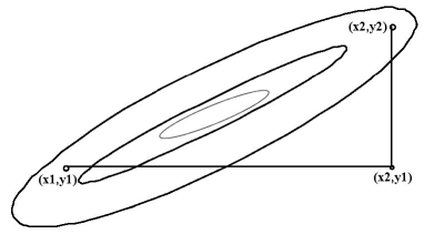
Figure 1: Crossover can generate points out of the attraction region.

To address this problem, in [30] was proposed another form of reproduction operator that was called linear crossover. From the two parent points $p_{1}$ and $p_{2}$ three new points are generated, namely:

$$\frac{1}{2}\left(p_{1}+p_{2}\right);\qquad\frac{3}{2}p_{1}-\frac{1}{2}p_{2};\qquad-\frac{1}{2}p_{1}+\frac{3}{2}p_{2}.\quad$$

The best two of these three points are selected.

Inspired on the above analysis we propose the algorithm of section 3.1 to learn a linear operator from a set $S$ of example functional points.

3 Applying GAs for Quantum Computing

3.1 GA for Learning Operators

Let us suppose that we do not know an operator $F:V\rightarrow V$ but, instead, we have a set of functional points $S=\left\{\left(\mid\chi_{i}\rangle,\mid\psi_{i}\rangle\right);\quad F\mid\chi_{i}\rangle=\mid\psi_{i}\rangle,\quad i=0,1,...,n-1\right\},$ where $\dim\left(V\right)=n$, also called the learning sequence. We can hypothesize a function $G$ such that $\left\|G\mid\chi_{i}\rangle-\mid\psi_{i}\rangle\right\|\cong 0$ (as usual, $\left\|\mid v\rangle\right\|=\sqrt{\langle v\mid v\rangle}$ is the norm induced by the inner product).

In this section, we present our general learning algorithm, based on GAs, to find $G$ [6]. This work was motivated by Dan Ventura’s algorithm for learning quantum operators [28], which resembles basic methods in neural networks [2]. Our GA method has a range of applications larger than that one of Dan Ventura’s learning algorithm. This is the main contribution of the work described next.

Following [30], each population member (chromosome) is a matrix $A\in\Re^{n\times n}$, and alleles are real parameters (matrix entries). The alleles are restricted to $\left[-1,1\right]$, but more general situations can be implemented.

The initial population is randomly generated. Once a population is obtained, a fitness value is calculated for each member. The fitness function is defined by:

$$fitness\left(A\right)=\exp\left(-error\left(A\right)\right);\quad A\in\Re^{n\times n},$$ (13)

where the error function is defined as follows. Let the learning sequence $S=\left\{\left(\mid\chi_{i}\rangle,\mid\psi_{i}\rangle\right);\quad i=1,...,m\right\}$ , then:

$$error\left(A\right)=\frac{1}{n\cdot m}\sum_{i=1}^{m}\left\|A\mid\chi_{i}\rangle-\mid\psi_{i}\rangle\right\|_{1},$$ (14)

where $\left\|x\right\|_{1}$ denotes the 1-norm of a $x=\left(x_{1},...,x_{n}\right)$, defined by: $\left\|x\right\|_{1}=\left|x_{1}\right|+...+\left|x_{n}\right|.$

Once the fitness is calculated for each member, the population is sorted into ascending order of the fitness values. Then, the GA loop starts. Before enter the loop description, some parameters must be specified.

Population Size: Number of individuals in each generation ($N$).

Elitism: It might be convenient just to retain some number of the best individuals of each population (members with best fitness) ($Ne$). The other ones will be generated through mutation and/or crossover. This kind of selection method was first introduced by Kenneth De Jong [16] and can improve the GA performance.

Selection Pressure: The degree to which highly fit individuals are allowed many offsprings [16] ($Ps$). For instance, for a selection pressure of $0.6$ and a population with size $N$, we will get only the $0.6*N$ best chromosomes to apply genetic operators.

Mutation Number: Maximum number of alleles that can undergo mutation ($Nm$). We do not choose to make mutations (implemented as perturbations) in $\Re^{n\times n}$, likewise in [30]. Instead, we randomly choose some matrix entries to be perturbed.

Termination Condition: Maximum number of generations ($Ngen$).

Mutation and Crossover Probabilities: $Pm$ and $Pc$, respectively.

The crossover is defined as follows. Given two parents $A=\left[a_{ij}\right]$ and $B=\left[b_{ij}\right]$  the following steps are performed until two offspring $C_{1},C_{2}$ are generated: (1) Randomly choose one of the parents; (2) Take a $(ij)$ matrix entry and puts its value on $c_{ij}$. Go to step (1).

The mutation is implemented as a perturbation of the alleles. Thus, given a member $A$, the mutation operator works as follows: $A\rightarrow A+\Delta$; where $\Delta$ is a perturbation matrix. The mutation number establishes the quantity of non-null entries for $\Delta.$ They are defined according to the mutation probability and a pre-defined Perturbation Size, that is, a range $\left[a,b\right]\in\Re$, such that $a\leq\Delta_{ij}\leq b$.

Once the above parameters are pre-defined and the input set ($S$) is given, the GA algorithm proceeds. In the following pseudo-code block, $P\left(t\right)$ represents the population at the interaction time $t$ and $N$ is its size. $Ngen$ is the maximum number of generations allowed, the procedure $Evaluate\_Sort$ calculates the fitness of each individual and sort the chromosomes into ascending order of the fitness values. The integer $Ne$ defines de elite members, the parameter $Ps\in\left[0,1\right]$ defines the selection pressure and $Nm$ the number of matrix entries that may undergo mutations.

Procedure Learning-GA
$t\leftarrow 0$;
initialize $P\left(t\right)$;
while($t<Ngen$) do

$t\leftarrow t+1$;

$Evaluate\_Sort\left(P\left(t-1\right)\right)$;

Store in $P\left(t\right)$ the $Ne$ best members of $P\left(t-1\right)$;

Complete $P\left(t\right)$ by crossover and mutation;
end while

3.1.1 Experimental Results

Firstly, we analyze the behavior of the GA learning algorithm for the same example presented in [28]. The set $S$ is given by:

$$S=\left\{\begin{array}[]{l}\left(\frac{1}{\sqrt{5}}\left[\begin{array}[]{l}2\\ 1\end{array}\right],\frac{1}{\sqrt{10}}\left[\begin{array}[]{l}3\\ 1\end{array}\right]\right)\\ \left(\frac{1}{\sqrt{20}}\left[\begin{array}[]{l}-2\\ 4\end{array}\right],\frac{1}{\sqrt{40}}\left[\begin{array}[]{l}2\\ -6\end{array}\right]\right)\end{array}\right\},$$ (15)

and the target is the Hadamard Transform $H$, defined by expression (8).

The GA result over $25$ runs was always the correct one. The set of parameters is given in the first line of Table 1. The perturbation size is given by $\left[0.001,0.1\right]$.

Matrix	$Ngen$	$N$	$Pc$	$Pm$	$Ps$	$Ne$	$Nm$
$2\times 2$	$100$	$200$	$0.85$	$0.95$	$0.30$	$30$	$1$
$2\times 2$	$200$	$200$	$0.85$	$0.95$	$0.30$	$30$	$1$

Table 1: Parameters for the examples of this section (definitions on section 3.1).

Figure 2 shows the error evolution over the $25$ runs. We collect the best population member (smallest error) for each run and take the mean value, for each generation, over the $25$ runs. It suggests that the algorithm gets closer the solution fast but takes much more time to achieve the target. Indeed, this behavior was observed for all experiments reported in [8].

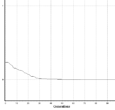
Figure 2: Error evolution, over $25$ runs, for example given by expression (15).

Dan Ventura’s algorithm gives also the correct result for this example, as reported in [28].

Now, let us take the following set $S$:

$$S=\left\{\begin{array}[]{l}\left(\frac{1}{\sqrt{5}}\left[\begin{array}[]{l}1\\ 2\end{array}\right],\frac{1}{\sqrt{10}}\left[\begin{array}[]{l}3\\ -1\end{array}\right]\right)\\ \left(\frac{1}{\sqrt{2}}\left[\begin{array}[]{l}1\\ 1\end{array}\right],\frac{1}{\sqrt{4}}\left[\begin{array}[]{l}2\\ 0\end{array}\right]\right)\end{array}\right\}.$$ (16)

In this set, the input vectors are not orthonormal ones. Thus, as we demonstrate in [6], if we apply Ventura’s algorithm we get a result which is far from the target (see [8] for more details). But, our GA algorithm was able to deal with this case. The operator to be learned is the Hadamard Transform, as before.

The second line of Table 1 shows the parameters used. We would like to keep all parameters unchanged but the number of generations ($Ngen$) had to be increased to achieve the correct result. This point out that our GA method may be sensitive to the fact that the set $\left\{\mid\chi_{0}\rangle,\mid\chi_{1}\rangle\right\}$ is not an orthonormal basis, despite that it learns correctly. Additional examples must be performed in order to verify this observation.

The mean error evolution shows a behavior which is similar to the first example. It decays fast but takes some time to become null.

Table 1 shows that we could keep the crossover and mutation probabilities unchanged for both these experiments (more results are presented on [8]). It is desired because it may indicates some parameter stability. Moreover, the clock time for one run is very acceptable ($\leq 0.04$ seconds).

3.2 GA for Quantum Circuit Design

Despite of the scientific and technological importance of quantum computation, few quantum algorithms faster then the classical ones have been discovered. Shor’s algorithm for quantum factoring, Grove’s quantum search and Deutsch-Jozsa algorithm are basically the known ones [14, 19].

This is due to the fact that the generation of such algorithms or circuits is difficult for a human researcher. They are unintuitive, mainly due to quantum mechanics features like entanglement and collapse (section 2.1). That is way researchers have investigated the use of stochastic search techniques, such as genetic programming and genetic algorithms to help in this task.

Among the main works in this subject [31, 23, 29, 27], those ones proposed in [31] and [23] are closer to our current research in this field.

The paper [23] presents a new representation and corresponding set of genetic operators for a scheme to evolve quantum circuits. A quantum circuit is represented as a list of structures (gate structures), where the size of a circuit (number of gates) can vary up to a pre-defined maximum number. Each gate structure contains the gate type, which is one in an allowable set of gate types including the usual Identity, CNOT, Hadamard and measurement operators, and a binary string for each category of qubit and parameter for that gate (see Figure 3).

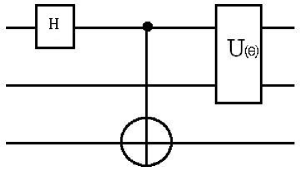
(a)

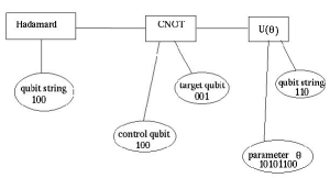
(b)

Figure 3: (a) Quantum Circuit. From the left to right:Hadamard ($H$), CNOT and the Rotation Gate $U\left(\theta\right)$. (b) The corresponding representation.

The crossover and mutation operators are defined as follows. Crossover operates on all the levels of an individual’s structure: the gates, qubit operands and parameter type. Gate crossover between two parent circuits consists of picking a gate from each parent at random, and then swapping all gates between the parents after these two points. Crossover between binary strings representing parameters can only occur between strings of like category, and proceeds in the same way as the crossover operator for the fixed length GA: pick a crossing point, and then swap bit values between the two strings after the point.

Mutation happens in the gate level. A gate is mutated by replacing it with a new one randomly selected. Mutation is performed with small probability (typically 0.001) because in [23] mutation is considered more an insurance against loss of important building blocks than a fundamental search procedure. Such viewpoint may be changed for circuit optimization. We shall return to this point ahead.

An error function is defined to compare the stored state(s) with the desired one(s): Given a set of cases consisting of input states and desired outputs, the error is defined by $error=\sum_{i,j}\left|\sigma_{ij}-d_{ij}\right|$, where we take for each case $i$, the sum of the magnitudes of the differences between the probability amplitudes of the desired result $d_{i}$ and that obtained one $\sigma_{i}$. A fitness function is constructed based on this error [23]. The production of entangled states was the focused application.

Reference [31] is another proposal in the application of GAs for quantum circuit design. The philosophy is similar to the one presented above.

The case study is the teleportation circuit [5]. Quantum teleportation is a technique by which a quantum state can be transported from one point to another through non-local interactions [4]. To illustrate the steps involved in quantum teleportation let us consider that there are two friends, Alice and Bob.

Imagine that Alice wants to deliver a qubit $\mid f\rangle=p\mid 0\rangle+q\mid 1\rangle$  to Bob, who lives far apart. Alice does not know $p$ and $q.$ Moreover, she can not have access to these values by measuring the qubit because, according to the quantum mechanics postulates, the system will collapse to a state $p/\left|p\right|\mid 0\rangle$ or $q/\left|q\right|\mid 1\rangle$.  Once measurement is an irreversible task, the information would be lost.

The scheme to solve this problem comprises the quantum teleportation. Its physical basis was proposed by Bennet et al. [4], followed by Brassard [5], who proposed the quantum circuit of Figure 4 for teleporting a single qubit.

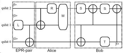
Figure 4: Brassard’s circuit for teleporting a single qubit.

In the circuit of Figure 4, we have the following components: quantum gates $L,$ $R,$ $S,$ $T$, given by:

$$L=\frac{1}{\sqrt{2}}\left[\begin{array}[]{cc}1&-1\\ 1&1\end{array}\right],\quad R=\frac{1}{\sqrt{2}}\left[\begin{array}[]{cc}1&1\\ -1&1\end{array}\right],$$ (17)

$$S=\left[\begin{array}[]{cc}i&0\\ 0&1\end{array}\right],\quad T=\left[\begin{array}[]{cc}-1&0\\ 0&-i\end{array}\right],$$ (18)

measurement operator $M$ and the CNOT gate, already defined in expression (11), and represented like in Figure 3.

The circuit has $3$ qubits, namely qubit $0,1$ and $2$, from the bottom to the top of the circuit. The method explores the concept of entanglement by using the EPR state given in equation (4). The first part of the circuit is used to create that kind of entangled state. In this operation, the zeroth and first qubits are affected. The input state is given by the tensor product $\mid f\rangle\mid 0\rangle\mid 0\rangle$ and the computation performs as follows:

$$I\otimes L\otimes I\mid f\rangle\mid 0\rangle\mid 0\rangle=\mid f\rangle\left(\frac{\mid 0\rangle+\mid 1\rangle}{\sqrt{2}}\right)\mid 0\rangle=\mid f\rangle\left(\frac{\mid 0\rangle\mid 0\rangle+\mid 1\rangle\mid 0\rangle}{\sqrt{2}}\right)$$

Then, by applying the $CNOT_{01}$; that is, the CNOT gate, defined by equations (11), with the first qubit as the control one, we find:

$$I\otimes CNOT_{01}\left[\mid f\rangle\left(\frac{\mid 0\rangle\mid 0\rangle+\mid 1\rangle\mid 0\rangle}{\sqrt{2}}\right)\right]=\mid f\rangle\left(\frac{\mid 0\rangle\mid 0\rangle+\mid 1\rangle\mid 1\rangle}{\sqrt{2}}\right)\equiv\mid f\rangle\mid\beta_{00}\rangle,$$ (19)

where $\mid\beta_{00}\rangle$ is the Bell state defined in expression (4). Similarly, the Alice’s circuit operates on the state given by expression (19). The result has the general form:

$$\mid\psi\rangle_{After-Alice}=\sum_{i,j,k\in\{0,1\}}a_{i,j,k}\mid ijk\rangle,$$ (20)

Then, Alice measures the first and second qubits. Thus, the state just after the measurement will be one of the:

$$\mid \psi\rangle_{0}=a_{000}\mid 000\rangle+a_{001}\mid 001\rangle;\quad\mid\psi\rangle_{2}=a_{100}\mid 100\rangle+a_{101}\mid 101\rangle;$$

$$\mid \psi\rangle_{1}=a_{010}\mid 010\rangle+a_{011}\mid 011\rangle;\quad\mid\psi\rangle_{3}=a_{110}\mid 110\rangle+a_{111}\mid 111\rangle.$$

Each result will be processed by Bob’s part. If we trace each measurement result we can confirm that the initial state of the second qubit was delivered to the zeroth qubit, which belongs to Bob. For instance, let us suppose that the result was $\mid\psi\rangle_{0}$ given above. Then, Bob’s circuit will outputs the following state [31]:

$$\left(\mid 0\rangle\mid 0\rangle-\mid 1\rangle\mid 0\rangle\right)\left(p\mid 0\rangle+q\mid 1\rangle\right)\equiv\left(\mid 0\rangle\mid 0\rangle-\mid 1\rangle\mid 0\rangle\right)\mid f\rangle,$$

which is a desired one, once the state of the second qubit was delivered to the zeroth; that is, it was teleported. The final state of the second qubit is different from the original one, which is accordance with the non-cloning theorem of quantum mechanics [19].

Once we have a quantum circuit (Figure 4) that performs the required computation, an interesting question arises: Given that quantum circuit how to find another one which performs the same computation but has less elementary gates? This optimization problem was addressed in [31] through genetic algorithms (GAs).

In fact, in [31], a circuit for quantum teleportation is encoded by a chromosome that is a string of integers chosen from the set $\left\{0,1,2,3\right\}.$ Each gene is interpreted with a codon, i.e., a three-letter unit. The first letter indicates a kind of gate, whereas the second and the third letters indicate the qubits that the gate will operate. For instance, let us consider the following string:

$$112\cdot 231\cdot 001\cdot\mathbf{3}31\cdot 132\cdot 012\cdot 122\cdot\mathbf{3}02\cdot 203\cdot 220\cdot 020\cdot 001$$ (22)

The first codon whose first letter is $3$ is interpreted as the partition between EPR-pair generation and Alice’s part. The second codon whose first letter is $3$ corresponds to Alice’s measurement. The codification used in [31] is defined by Tables 2 and 3:

	0	1	2	3
0	$CNOT_{01}$	$CNOT_{10}$			0
0	$CNOT_{01}$	$CNOT_{10}$			1
0	$CNOT_{01}$	$CNOT_{10}$			2
0					3
1	$L_{0}$	$L_{1}$			0
1	$L_{0}$	$L_{1}$			1
1	$L_{0}$	$L_{1}$			2
1					3
2	$R_{0}$	$R_{1}$			0
2	$R_{0}$	$R_{1}$			1
2	$R_{0}$	$R_{1}$			2
2					3
3	$\cdot$	$\cdot$	$\cdot$	$\cdot$	*

	0	1	2	3
0	$CNOT_{12}$	$CNOT_{21}$			0
0	$CNOT_{12}$	$CNOT_{21}$			1
0	$CNOT_{12}$	$CNOT_{21}$			2
0					3
1	$L_{1}$	$L_{2}$			0
1	$L_{1}$	$L_{2}$			1
1	$L_{1}$	$L_{2}$			2
1					3
2	$R_{1}$	$R_{2}$			0
2	$R_{1}$	$R_{2}$			1
2	$R_{1}$	$R_{2}$			2
2					3
3	$\cdot$	$\cdot$	$\cdot$	$\cdot$	*

Table 2: Codification for EPR generation (left). Alice’s gates codification (right).

	0	1	2	3
0		$CNOT_{10}$	$CNOT_{20}$		0
0	$CNOT_{01}$		$CNOT_{21}$		1
0	$CNOT_{02}$	$CNOT_{12}$			2
0					3
1	$L_{0}$	$L_{1}$	$L_{2}$		0
1	$L_{0}$	$L_{1}$	$L_{2}$		1
1	$L_{0}$	$L_{1}$	$L_{2}$		2
1					3
2	$R_{0}$	$R_{1}$	$R_{2}$		0
2	$R_{0}$	$R_{1}$	$R_{2}$		1
2	$R_{0}$	$R_{1}$	$R_{2}$		2
2					3
3	$\cdot$	$\cdot$	$\cdot$	$\cdot$	*

Table 3: Codons for Bob’s circuit generation.

This circuit representation is closer that one proposed in [23] (described above). However, differently from that reference, in this representation the same integer may have different meaning in different parts of the chromosome. For example, the letter $0$ means $CNOT_{01}$ during the EPR-pair generation while it means $CNOT_{12}$ for Alice’s part.

Once established the circuit representation, genetic operators based on mutations and crossover shall be specified. Mutations are implemented by properly change the alleles of a given chromosome. A two-point crossover is implemented by randomly choosing two parent chromosomes and exchange their alleles.

Finally, the following steps are executed: (1) Decode each chromosome in a circuit and its gates; (2) Apply these transformation on the initial state; (3) If the circuit outputs a final state similar to the desired one, its fitness is enlarged. (4) Apply the genetic operators to generate the next population; (5) Go to step (1).

Each individual (circuit) is evaluated as follows:

(1) Make three random numbers $\alpha,$ $\beta,$ $\gamma\in\left[0,2\pi\right].$

(2) Prepare three initial states $\left(p,q\right)$ given by: $\left(e^{i\beta}\cos\alpha,e^{i\gamma}\sin\alpha\right),$ $\left(e^{i\gamma}\cos\beta,e^{i\alpha}\sin\beta\right),\left(e^{i\alpha}\cos\gamma,e^{i\beta}\sin\gamma\right)$

(3) Derive the circuit by decoding the string using Tables 2 and 3.

(4) Use the state $\left(p\mid 0\rangle+q\mid 1\rangle\right)\otimes\mid 00\rangle$ as the input one.

(5) Evaluate the fitness.

(6) Change random numbers every 50 generations.

After the measurement, we have to trace all the branches. corresponding to the possible outcomes given by equations (3.2). The desired final state, at the end of Bob’s circuit has a general form $\left(a\mid 00\rangle+b\mid 01\rangle+c\mid 10\rangle+d\mid 11\rangle\right)\otimes\left(p\mid 0\rangle+q\mid 1\rangle\right)\equiv\left(ap,aq,bp,bq,cp,cq,dp,dq\right).$ Thus, the ratio $a_{i}/a_{i+1}=p/q;$ $i=0,2,4,6.$ This gives a clue to find out an efficient fitness function.

Given a circuit, we observe that each one of the initial states produces $4$ final states (one for each possible measurement’s result, given by expressions (3.2)). Thus, for the three initial states, we will have $12$ possible final states. If we write the final states as $\left(a_{j,0};a_{j,1};...,a_{j,7}\right)$, $j=0,2,..,11$, we can express the gap between a final state and the desired one as:

$$error_{j}=\frac{1}{n}\sum_{i=0,2,4,6}\left|\frac{a_{j,i}}{a_{j,i+1}}-\frac{p}{q}\right|,$$

where $n$ is the numbers of pairs such that $\left(a_{j,i},a_{j,i+1}\right)\neq\left(0,0\right)$ and the summation is taken over such pairs. In the case that the final state is $\mathbf{0}$ then $error_{j}$ is set to $100.$ The fitness function $f$ is defined as:

$$f=\frac{1}{1+10\sum error_{j}}.$$

If $f$ is $1,$ that is, if the circuit is correct, the bonus of $1/\left(number-of-gates\right)$ is added to $f$ so as to apply a selection pressure based upon the circuit size (fitness is enlarged).

In [31] authors used the roulette-wheel selection and two-point crossover with probability $0.7$. Differently from the work found in [23], for circuit design (section 3.2), mutation is considered more significant in this case. The mutation probability is $1/\left(chromosome-length\right)$; that is, the algorithm is biased in the preservation of smaller chromosomes against the larger ones. The population size and the maximum number of generations was $5,000$ and $1,000$, respectively. All individuals are replaced every generation (there is no elitism). The simpler circuit so obtained is pictured on Figure 5:

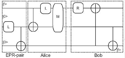
Figure 5: Optimized circuit for the quantum teleportation problem.

We can check that the circuit on Figure 5 is encoded by the string given by (22). This circuit has $8$ gates while Brassard’s had eleven (Figure 4), which demonstrate the capabilities of the GA procedure to evolve an initial circuit towards a simpler one.

We are in charge with an implementation of this algorithm, but using different strategies. We shall return to this point in section 5.

4 Quantum Evolutionary Computation

4.1 Quantum-Inspired Genetic Algorithms

In this section we present the second part of our review: the analysis of genetic algorithms based on quantum computing concepts. This is an important step towards the implementation of genetic algorithms in a quantum hardware.

We start with the Quantum-Inspired Genetic Algorithm (QIGA) proposed in [11]. The QIGA is characterized by principles of quantum computing including qubits and probability amplitude. It uses a qubit representation instead of the usual binary, numeric, or symbolic representations [15, 16]. More specifically, QIGA uses a m-qubit representation, defined as:

$$\left[\left(\begin{array}[]{l}\alpha_{10}\\ \alpha_{11}\end{array}\right),\left(\begin{array}[]{l}\alpha_{20}\\ \alpha_{21}\end{array}\right),...,\left(\begin{array}[]{l}\alpha_{m0}\\ \alpha_{m1}\end{array}\right)\right],$$ (23)

where each pair $\left(\alpha_{i0},\beta_{i1}\right);i=1,...,m$, indicates a qubit.

Now, we must explain how convergence can be obtained with the qubit representation. Let us consider the following scheme, which is proposed in [11].

For each m-qubit chromosome of the form (23), a binary string $\left\{x_{1},x_{2},...,x_{m}\right\}$ is defined, where each bit is selected using the corresponding qubit probability, $\left|\alpha_{i0}\right|^{2}$ or $\left|\alpha_{i1}\right|^{2}$. Observe that if $\left|\alpha_{i0}\right|^{2}$ or $\left|\alpha_{i1}\right|^{2}$ approaches to $1$ or $0$, the qubit chromosome converges to a single state and the diversity given by the superposition of states disappears gradually.

An application dependent fitness function is used to evaluate the solution $\left\{x_{1},x_{2},...,x_{m}\right\}$. Another step is to design efficient evolutionary strategies. This would be accomplished through crossover and mutations but their implementations are not explained in [11] . Obviously, as usual, we can suppose a one-point crossover between parent chromosomes as well as unitary operators to change a randomly chosen qubit $\left(\alpha_{i0},\beta_{i1}\right)$ of the expression (23). However, as the QIGA has diversity caused by the qubit representation, the role of genetic operators is not clear. Also, it is stated in [11] that, if the probabilities of mutation and crossover are high, the performance of the QIGA can be decreased notably.

At the beginning of the algorithm, a population $Q\left(t\right)=\left\{q_{1}^{t},q_{2}^{t},...,q_{m}^{t}\right\}$ of m-qubit chromosomes is instantiated. Given a m-qubit chromosome in $Q\left(t\right)$ we can find the corresponding binary string through the rule stated above. The so obtained binary string population will be denoted by $P\left(t\right).$

Besides, there is an update step which aims to increase the probability of some states. Henceforth, given a qubit $\left(\alpha_{i0},\alpha_{i1}\right)$ of a m-qubit chromosome, it is updated by using the rotation gate $U\left(\theta_{i}\right)$:

$$U\left(\theta_{i}\right)=\left[\begin{array}[]{cc}\cos\left(\theta_{i}\right)&-\sin\left(\theta_{i}\right)\\ \sin\left(\theta_{i}\right)&\cos\left(\theta_{i}\right)\end{array}\right];\quad\left[\begin{array}[]{c}\alpha_{i0}^{\prime}\\ \alpha_{i1}^{\prime}\end{array}\right]=U\left(\theta_{i}\right)\left[\begin{array}[]{c}\alpha_{i0}\\ \alpha_{i1}\end{array}\right],$$ (24)

where $\theta_{i}$ is formed through the binary solutions $P\left(t\right)$ and the best solution found (see next).

Let us present a pseudo-code of the QIGA developed in [11]:

Procedure QIGA

$begin$

$t\leftarrow 0$

      Initialize $Q\left(t\right)$

      Make $P\left(t\right)$ by observing $Q\left(t\right)$

      Evaluate $P\left(t\right)$

      Store the best solution $b$ among $P\left(t\right)$

$while$(not termination-condition) do

$begin$

$\qquad\qquad t\leftarrow t+1$

        Make $P\left(t\right)$ by observing $Q\left(t-1\right)$

        Evaluate $P\left(t\right)$

        Update $Q\left(t\right)$ using quantum gates $U\left(t\right)$

        Store the best solution $b$ among $P\left(t\right)$

$end$

$end$

The quantum gates $U\left(t\right)$ are application dependent. This step aims to improve the convergence. After updating $Q\left(t\right),$ the best solution among $P\left(t\right)$ is selected, and if the solution is fitter than the stored best solution, the stored solution is replaced by the new one. The binary solutions $P\left(t\right)$ are discarded at the end of the loop. A parallel version of the QIGA is presented in [12].

A significant point to be considered is the exploration of the tensor product to enlarge diversity. Despite of authors claim in [11], the scheme proposed did not take advantage of such effects at all. We will analyze this point in section 5.

4.1.1 Experiments for QIGA

The knapsack problem, which is a kind of combinatorial optimization problem [18], is used in [11] to investigate the performance of QIGA. The $0-1$ knapsack problem is described as: given a set of $m$ items and a knapsack with limited capacity $C$, select a subset of the items so as to maximize a profit function $f\left(x\right)$ given by:

$$f\left(x\right)=\sum_{i=1}^{m}p_{i}x_{i},$$ (25)

and subjected to:

$$\sum_{i=1}^{m}w_{i}x_{i}<C,$$ (26)

where $\left(x_{1},x_{2},...,x_{m}\right)\in\left\{0,1\right\}^{m}$, $p_{i}$ and $w_{i}$ are the profit and the weight associated to the item $i$, respectively.

When applying the QIGA to this problem, the length of a qubit chromosome is the same as the number of items. The $i-th$ item can be selected for the knapsack with probability $\left|\alpha_{i0}\right|^{2}$, following the procedure given in section 4.1. Thus, from each m-qubit chromosome a binary string of the length $m$ is formed. The binary string $x_{j}$ represents the $j-th$ candidate solution to the problem. The $i-th$ item is selected for the knapsack if and only if $x_{ij}=1.$ To measure the efficiency of the QIGA, its performance was compared with that one of conventional genetic algorithms (CGAs). Three types of CGAs were considered: algorithms based on penalty functions, algorithms based on repair methods, and algorithms based on decoders [11, 18].

For the first group of algorithms, the profit function is:

$$f\left(x\right)=\sum_{i=1}^{m}p_{i}x_{i}-Pen\left(x\right),$$ (27)

where $Pen\left(x\right)$ is a penalty function. Among the possibilities to define penalty functions the following ones were considered in [11]:

$$Pen_{1}\left(x\right)=\log_{2}\left(1+\rho\left(\sum_{i=1}^{m}w_{i}x_{i}-C\right)\right),$$ (28)

$$Pen_{2}\left(x\right)=\rho\left(\sum_{i=1}^{m}w_{i}x_{i}-C\right),$$ (29)

$$Pen_{3}\left(x\right)=\left(\rho\left(\sum_{i=1}^{m}w_{i}x_{i}-C\right)\right)^{2}.$$ (30)

where $\rho=\max\left\{p_{i}/w_{i};\quad i=1,...,m\right\}$.

For repair methods, the profit is defined by:

$$f\left(x\right)=\sum_{i=1}^{m}p_{i}x_{i}^{\prime},$$ (31)

where $x^{\prime}$ is a repaired vector of the original vector $x$. Original chromosomes are replaced with a $5\%$ probability in the experiment. The two repair algorithms considered in [11] differ only in selection procedure, which chooses an item for removal from the knapsack:

$Rep_{1}$(random repair): The selection procedure selects a random element from the knapsack.

$Rep_{2}$(greedy repair): All items in the knapsack are sorted in the decreasing order of their profit to weight ratios. The selection procedure always chooses the last item for deletion.

A possible decoder for the knapsack problem is based on an integer representation. Each chromosome is a vector of $m$ integers; the $i-th$ component of the vector is an integer in the range from $1$ to $m-i+1$. The ordinal representation references a list $L$ of items; a vector is decoded by selecting appropriate item from the current list. The two algorithms for this class used in [11] are:

$Dec_{1}$(random decoding): The build procedure creates a list $L$ of items such that the order of items on the list corresponds to the order of items in the input file which is random.

$Dec_{2}$(greedy decoding): The build procedure creates a list $L$ of items in the decreasing order of their profit to weight ratios.

Besides, there were an experiment that implements a scheme using $Pen_{2}$ and $Rep_{1}$.

The QIGA proposed in [11] for this problem contains a repair algorithm. It can be described as follows:

Procedure QIGA-Knapsack

$begin$

$t\leftarrow 0$

      Initialize $Q\left(t\right)$

      Make $P\left(t\right)$ by observing $Q\left(t\right)$

      repair $P\left(t\right)$

      Evaluate $P\left(t\right)$

      Store the best solution $b$ among $P\left(t\right)$

$while$($t<MAX\_GEN$) do

$begin$

$\qquad\qquad t\leftarrow t+1$

        Make $P\left(t\right)$ by observing $Q\left(t-1\right)$

        repair $P\left(t\right)$

        Evaluate $P\left(t\right)$

        Update $Q\left(t\right)$ using quantum gates $U\left(t\right)$

        Store the best solution $b$ among $P\left(t\right)$

$end$

$end$

Procedure make$\left(x\right)$

$begin$

$i\leftarrow 0$

$while$($i<m$) do

$begin$

$i\leftarrow i+1$

if $random\left[0,1\right]>\left|\alpha_{i0}\right|^{2}$

then $x_{i}\leftarrow 1$

else $x_{i}\leftarrow 0$

$end$

$end$

Procedure repair$\left(x\right)$

$begin$

knapsack-overfilled $\leftarrow$ false

if $\sum_{i=1}^{m}w_{i}x_{i}>C$

then knapsack-overfilled $\leftarrow$ true

while (knapsack-overfilled) do

$begin$

select an $i-th$ item from the knapsack

$x_{i}\leftarrow 0$

if $\sum_{i=1}^{m}w_{i}x_{i}\leq C$

then knapsack-overfilled $\leftarrow$ false

$end$

while (not knapsack-overfilled) do

$begin$

select a $j-th$ item from the knapsack

$x_{j}\leftarrow 1$

if $\sum_{i=1}^{m}w_{i}x_{i}>C$

then knapsack-overfilled $\leftarrow$ true

$end$

$x_{j}\leftarrow 0$

$end$

The profit of a binary solution is evaluated by expression (31) and it is used to find the best solution $b$ among $P\left(t\right)$. A m-qubit chromosome is updated by using the rotation gates, following expression (24). The angles $\theta_{i}$ are computed as follows. Let us suppose that we have a binary string $x=\left(x_{1},x_{2},...,x_{m}\right)$ such that $f\left(x\right)>f\left(b\right)$, where $f$ is defined by expression (31). If $x_{i}=1$ and $b_{i}=0$, the idea is to set the value of $\theta_{i}=sign\left(\alpha_{i0}\cdot\alpha_{i1}\right)\Delta\theta_{i}$ such that the probability amplitude of $\mid 1\rangle$ is increased. Thus, we want that $\left|\alpha_{i1}^{\prime}\right|^{2}>\left|\alpha_{i1}\right|^{2}$, where $\alpha_{i1}^{\prime}$ is given by equation (24). So:

$$\left|\alpha_{i1}^{\prime}\right|^{2}=\left(\alpha_{i0}\sin\theta_{i}+\alpha_{i1}\cos\theta_{i}\right)^{2}=\left(\alpha_{i0}\sin\theta_{i}\right)^{2}+\left(\alpha_{i1}\cos\theta_{i}\right)^{2}+2\alpha_{i0}\alpha_{i1}\sin\theta_{i}\cos\theta_{i},$$ (32)

where we have supposed that $\alpha_{i0},\alpha_{i1}$ are real ones for simplicity. Thus, to increase the desired probability amplitude as much as possible we should set $sign\left(\alpha_{i0}\cdot\alpha_{i1}\right)=+1,-1,0,$ according to $\alpha_{i0}\alpha_{i1}>0,$ $\alpha_{i0}\alpha_{i1}<0,$ or $\alpha_{i0}\alpha_{i1}=0$, respectively. The setting of $\Delta\theta_{i}$ is through experimentation. In the reported example, it was set to $0.025$. Following such procedure, a lookup table for $\theta_{i}$ can be performed (see [11] details).

The update procedure is given bellow:

Procedure update$\left(q\right)$

$begin$

$i\leftarrow 0$

while ($i<m$) do

$begin$

$i\leftarrow i+1$

determine $\theta_{i}$

obtain $q^{\prime}=\left(\alpha_{i0}^{\prime},\alpha_{i1}^{\prime}\right)$ as:

$\left(\alpha_{i0}^{\prime},\alpha_{i1}^{\prime}\right)^{T}=U\left(\theta_{i}\right)\left(\alpha_{i0},\alpha_{i1}\right)^{T}$

$end$

$q\leftarrow q^{\prime}$

$end$

The results obtained by the QIGA just presented, reported in [11], uses the following profits and weights:

$$w_{i} = uniformly-random[1,10),$$ (33)

$$pi = w_{i}+5.$$

The average knapsack capacity was used:

$$C=\frac{1}{2}\sum_{i=1}^{m}w_{i}.$$ (34)

The data files were unsorted and the number of items were $100,$ $250$ and $500$.

The population size of the eight conventional genetic algorithms was equal to $100$. Probabilities of crossover and mutation were fixed: $0.65$ and $0.05$, respectively. The population size is $1$, for the first series of experiments, and $10$ for the second one. As a performance measure of the algorithm the best solution found within $500$ generations over $25$ runs is collected. Also, the elapsed time per one run is checked.

For $100$ items QIGAs yielded superior results as compared to all the CGAs. For $250$ and $500$ items the QIGA with $10$-size population outperforms all the classical ones [11].

4.2 Quantum Genetic Algorithms

The work reported on section 4.1 shows that the application of quantum computing concepts to evolutionary programming is a promising research. The results presented points out that a quantum genetic algorithm (QGA) would outperform the classical ones. Besides, such implementation would take advantage of quantum parallelism as well as GAs parallelism. The obvious question is how to implement genetic algorithms in quantum computers?

The reference [25] is an effort to produce a QGA. Despite of the fact that there are several open points, it is the first effort in the direction of such algorithm.

The QGA proposed in [25] uses two registers for each quantum individual; the first one stores an  individual while the second one stores the individual’s fitness. These two registers are referred as individual register and the fitness register, respectively. A population of $N$ quantum individuals is stored through pairs of registers $\left(individual-register_{i},fitness-register_{i}\right)$, $i=1,..,N$.

At different times during the QGA the fitness register would store a single fitness value or a quantum superposition of fitness values. Identically for the individual register.

Once a new population is generated, the fitness for each individual would be calculated and the result stored in the individual ’s fitness register.

The effect of the fitness measurement is a collapse given by expression (6). This process reduces each quantum individual to a superposition of classical individuals with a common fitness. It is a key step in the QGA [25]. Then, crossover and mutation would be applied. The whole algorithm can be written as follows:

Quantum Genetic Algorithm

Generate a population of quantum individuals.

Calculate the fitness of the individuals.

Measure the fitness of each individual (collapse).

$while$(termination-condition) do

Selection based on the observed fitness.

Crossover and Mutations are applied.

Calculate the fitness of the individuals.

Measure the fitness of each individual (collapse).

$end\quad while$

According to [25], the more significant advantage of QGA’s will be an increase in the production of good building blocks (schemata [13, 16]) because, during the crossover, the building block is crossed with a superposition of many individuals instead of with only one in the classical GAs.

One can also view the evolutionary process as a dynamic map in which populations tend to converge on fixed points in the population space. From this viewpoint the advantage of QGA is that the large effective size allows the population to sample from more basins of attraction. Thus, it is much more likely that the population will include members in the basins of attraction for the higher fitness solutions.

Another advantage is the quantum computer’s ability to generate true random numbers. By applicating Kolmogorov complexity analysis, it has been shown that the output of classical implementations in genetic programming, which use a pseudo random number generator, are bounded above by the genetic programming itself, whereas with the benefit of a true random number generator there is no such bound [25, 24].

Despite of these promising features, fundamental points are not addressed in [25]. Firstly, it is not clear how to implement crossover in a quantum computers. Besides, how to perform the fitness function calculation in quantum hardware? Even a much more fundamental problem is that to explore the superposition of quantum individuals the correlation $individual\leftrightarrow fitness$ must be kept during the whole computation. Entanglement seems to be the only possibility to accomplish this task. But, in this case, things must be formally described to avoids misunderstandings and wrong interpretations. We develop such mathematical formalism on section 5.

5 Discussion and Perspectives

In this section we analyze some issues concerning to the reviewed methods. Possible solutions and perspectives in this area are also discussed.

In [8] we show some challenges concerning the GA for learning linear operators (section 3.1). Other tests presented in [8] show that the number of generations seems to increase when space dimension gets higher. The increasing rate must be controlled if we change the population size properly. However, such procedure could be a serious limitation of the algorithm for large linear systems.

The behavior for underconstrained problems; that is, when $S=\left\{\left(\mid\chi_{i}\rangle,\mid\psi_{i}\rangle\right);\quad F\mid\chi_{i}\rangle=\mid\psi_{i}\rangle,\quad i=1,...,K<n\right\},$ where $n$ is the space dimension, is also analyzed in [8]. In this case, we had to increase the population size but the number of generations is smaller than that one for the constrained test ($K=n$). As we expect, there is a trade-off between the increase of solutions and the fact that we are less able to properly evolve the populations due to the lack of prior information. Moreover, the observed success is an advantage of the method, if compared with traditional ones. In this case, numerical approaches based on iterative methods in matrix theory (Gauss-Seidel, GMRES, etc) can not be applied without extra machinery because the solution is not unique [8].

The comparison with Dan Ventura’s learning method, given on section 3.1.1, shows that our algorithm overcomes the limitation of the later: we do not need that $\left\{\mid\chi_{0}\rangle,\mid\chi_{1}\rangle\right\}$ is an orthonormal basis of the vector space. However, when using our GA method, we pay a price due to storage requirements and computational complexity.

Dan Ventura’s algorithm as well as numerical methods (see [8] and references therein), have a computational cost asymptotically limited by $O\left(n*n^{2}\right)$ while our GA method needs $O\left(Ngen*N*n^{2}\right)$ float point operations. Besides, for traditional numerical methods and Ventura’s algorithm, we observe a storage requirements of $O\left(n^{2}\right)$ against $O\left(N*n^{2}\right)$ for our approach. Thus, the disadvantage of our method becomes clear.

However, if compared with matrix methods, our algorithm is in general less sensitive to roudoff errors [10]. This is due to, unlikely numerical methods that try to follow a path linking the initial position to the optimum, our GA algorithm searches the solution through a set of candidates.

To improve the convergence we need better evolutionary (crossover/mutation) strategies. The behavior pictured on Figure 2, of section 3.1.1, is a typical one for every test we made [8]. It indicates that our evolutionary strategies are efficient to get closer the solution but not to complete the learning process. Further analysis should be made to improve these operators.

When comparing the works for quantum circuit design, [23] and [31], we observe the following aspects:

1) Gate representation: The gate structure of [23] versus the codon used in [31]. Despite of some apparent difference between them, it is simple to check that they are equivalent, in the sense that, any gate can be represented with either the later or the former.

2) Genetic Operators: Both implementations have used crossover and mutations. However, the crossover implementation used in [23] operates on all the levels of an individuals structure (the gates, each category of qubit operands and each parameter type) while in [31] it affects only the gate and qubit levels. Mutations are basically equivalent because, if the alleles are randomly changed, like in [31], we are randomly replacing a gate with a new one, like in [23], and vice-versa.

3) Range of Applications: Despite of the fact that the aim of [31] is circuit optimization, it can be straightforwardly adapted for circuit design. This can be accomplished by changing the mutation probability (the formula $1/\left(chromosome-length\right)$ does not make sense in this case). We can follow [23] and set this probability to a small value (typically $0.001$). Besides, the fitness function remains case dependent and we stop using the bonus $1/\left(number-of-gates\right)$ to bias the solution to smaller circuits (if we do not know any prior correct circuit, there is no sense for prefering smaller circuits over bigger ones during evolution). Besides, some elitism may be introduced. Now, we are analyzing such modifications.

Moreover, a more fundamental question about GAs for circuit design follows from the next comments. The algorithms [23, 31] basically evolve an initial population of individuals towards a desired circuit. Evolution can be regarded as the exploration of search spaces by populations. Thus, an interesting question in this case is what about the structure of such spaces for circuit designing/optimization?

For instance, we must observe that without the identity operator the circuit size (number of gates) will be a variable. Henceforth, a search space of $12$-codons strings (like expression (22)), would be transformed in another one with just $8$-codons strings at the end of the optimization process. This can be seen as an evolutionary process called innovation [26].

Following [26] we do need a mathematical representation in which the kind and number of codons follow from the dynamics of the model. In [26] the concept of configuration spaces is proposed as one of such approach. Obviously, the Identity operator is a simple trick to address this problem if we know in advance the maximum circuit size. However, the concept of configuration spaces might open possibilities to analyze the structure of the circuit space. That is way we are going to consider this mathematical framework in our research.

A configuration space is a set of objects (circuits, for example) as well as a topological structure on this set which describes how these objects can be transformed into each other by an operator [26].

Symmetries of the configuration space induced by evolutionary mechanisms (mutation and crossover, for instance) are fundamental elements in this framework. They define the dimensionality of the space in which evolution occurs. Hence, any evolutionary process that affects the symmetries of the configuration space may change its dimensionality (the number of non-identity gates, in our case). The configuration space formalism includes beautiful mathematical results in finite Abelian groups [26]. We wish to analyze the algorithms proposed in [23, 31] through this formalism, in order to derive more efficient evolutionary strategies.

When considering the QIGA presented on section 4.1, some explanations must be offered about the diversity that can be achieved by the m-qubit representation [11].

Thus, let us take the make$\left(x\right)$ procedure. For simplicity, we are going to consider a $3$-qubit chromosome. Let $r_{1},r_{2},r_{3}$ be the random numbers generated during the $while$ loop execution in make$\left(x\right)$. We could have $r_{1}>\left|\alpha_{10}\right|^{2},r_{2}>\left|\alpha_{20}\right|^{2},r_{3}<\left|\alpha_{30}\right|^{2}$. Thus, the generated string would be $\left(1,1,0\right)$.

Now, consider the tensor product

$$\mid\psi_{1}\rangle\otimes\mid\psi_{2}\rangle\otimes\mid\psi_{3}\rangle=\sum_{i_{1},i_{2},i_{3}\in\left\{0,1\right\}}\alpha_{1i_{1}}\alpha_{2i_{2}}\alpha_{3i_{3}}\mid i_{1}\rangle\otimes\mid i_{2}\rangle\otimes\mid i_{3}\rangle.$$ (35)

Thus, the qubit chromosome will be represented as a superposition of the states $\mid i_{1}\rangle\otimes\mid i_{2}\rangle\otimes\mid i_{3}\rangle,\quad i_{1},i_{2},i_{3}\in\left\{0,1\right\}$, and so it carries information about all of them at the same time. Such observation points out the fact that the qubit representation has a better characteristic of diversity than classical approaches, since it can represent superposition of states. In classical representations we will need at least $2^{3}$ chromosomes to keep the information carried by expression (35) while only one 3-qubit chromosome is enough.

However, the probability amplitude of the state $\mid 1\rangle\otimes\mid 1\rangle\otimes\mid 0\rangle$ may not be the largest one. Henceforth, it does not seems that the binary string generation rule proposed in [11] does explore such diversity in general.

However, if we take another generation rule, say: if $\left|\alpha_{i1}\right|^{2}>\left|\alpha_{i0}\right|^{2}$ then $x_{i}\leftarrow 1$, else $x_{i}\leftarrow 0$, thus we can be sure that the generated binary string is an index to the larger amplitude probability of state (35). Experiments must be performed in order to show the efficiency of such rule.

The QGA presented in [25] exploits the quantum effects of superposition and entanglement. However, the lack of a more formal explanation raises some questions. How to implement crossover in quantum computers? How to compute the fitness function? What about a mathematical definition of a quantum individual? These are examples of such questions.

Now, we address some of these points in order to be closer to answer the question: what GAs will look like as an implementation on quantum hardware?

The starting point of our development comes from the known problem of finding the period $r$ of a periodic function $f:Z_{N}\rightarrow Z$, where $Z_{N}$ denotes the additive group of integers modulo $N$.

In this case, the quantum solution provided by Shor [19] uses a hardware with two registers in the following entangled state:

$$\mid\Psi\rangle=\frac{1}{\sqrt{N}}\sum_{x=0}^{N-1}\mid x\rangle\otimes\mid f\left(x\right)\rangle.$$ (36)

Thus, according to the expression (6), by measuring the second register, yielding, say, a value $y_{0}$, the first register ’s state will collapse to an uniform superposition of all those $\mid x\rangle^{\prime}s$ such that $f\left(x\right)=y_{0}$; that is:

$$\mid\Psi\rangle_{after}=\frac{1}{\sqrt{K}}\sum_{k=0}^{K-1}\mid x_{0}+kr\rangle,$$ (37)

where $x_{0}$ is such a $x$ and $N=Kr$. When using the state $\mid\Psi\rangle,$ given by expression (36), the desired effect is to keep the correspondence between each integer $x$ with its corresponding value $f\left(x\right)$.

Now, let us return to the QGA of section 4.2 and present a physical description of it. The quantum individual could be mathematically represented by a state given by expression (36), where $\mid x\rangle$ represents an individual and $f\left(x\right)$ its fitness. Thus, we keep the idea of representing a quantum individual through two registers which was used in [25]. So, if we have $M$ quantum individuals in each generation we need $M$ register pairs (individual register, fitness register).

In our formulation, each register is a closed quantum system. Thus all of them can be initialized with the state given by expression (36). Then, unitary operators $W$ will be applied in order to complete the generation of the initial population. Henceforth, the initialization could encompass the following steps:

1) For each register $i,$ generate the state:

$$\mid\varphi\rangle_{i}=\frac{1}{\sqrt{N}}\sum_{x=0}^{N-1}\mid x\rangle_{i}\otimes\mid 0\rangle_{i},\quad i=1,...,M,$$

2) Apply unitary operators $W$ (rotations, for example) and $U_{f}$, the known black box which performs the operation $U_{f}\mid a\rangle\otimes\mid 0\rangle=\mid a\rangle\otimes\mid f\left(a\right)\rangle$ [19], to complete the initial population:

$$\mid\Psi\rangle_{i}\equiv U_{f}W\mid\varphi\rangle_{i}=\sum_{x=0}^{N-1}U_{f}\left(W\left(\frac{\mid x\rangle_{i}}{\sqrt{N}}\right)\otimes\mid 0\rangle_{i}\right)=$$

$$=\sum_{x=0}^{N-1}U_{f}\left(a_{x}\mid x\rangle_{i}\otimes\mid 0\rangle_{i}\right)=$$

$$=\sum_{x=0}^{N-1}a_{xi}\mid x\rangle_{i}\otimes\mid f\left(x\right)\rangle_{i},\quad i=1,...,M.$$ (38)

We must highlight that all the above operations are unitary ones, consequently, can be performed in quantum computers [20]. Besides, it is important to observe that the fitness is stored in the second register after the generation of the population. Now, by measuring the fitness, each individual undergoes collapse, according to the expression (37):

$$\mid\Psi\rangle_{i}^{after}=\frac{1}{\sqrt{K_{i}}}\sum_{k=0}^{K_{i}-1}\mid k\rangle_{i}\otimes\mid y_{0}\rangle_{i},$$ (39)

where $\mid k\rangle_{i}$ is such that the observed fitness for the $i-th$ register is $f\left(k\right)=y_{0}$.

When entering the main loop, the observed fitness is used to select the best individuals. Then, genetic operators must be applied.

Mutations can be implemented through the following steps.

1) Apply $U_{f}^{-1}$ over the measurement result:

$$U_{f}^{-1}\mid\Psi\rangle_{i}^{after}=\frac{1}{\sqrt{K_{i}}}\sum_{k=0}^{K_{i}-1}\mid k\rangle_{i}\otimes\mid 0\rangle_{i},$$ (40)

2) Unitary operators $P$ (small rotations, for example) are applied to the above result:

$$P\left(U_{f}^{-1}\mid\Psi\rangle_{i}^{after}\right)=\sum_{k=0}^{K_{i}-1}P\left(\frac{\mid k\rangle_{i}}{\sqrt{K_{i}}}\right)\otimes\mid 0\rangle_{i}=$$

$$=\sum_{x=0}^{N-1}\beta_{xi}\mid x\rangle_{i}\otimes\mid 0\rangle_{i},$$ (41)

where we expanded the result in the computational basis.

3) Finally, apply $U_{f}$ to recover the diversity that was lost during the measurement:

$$U_{f}PU_{f}^{-1}\mid\Psi\rangle_{i}^{after}=\sum_{x=0}^{N-1}\beta_{xi}\mid x\rangle_{i}\otimes\mid f\left(x\right)\rangle_{i}.$$ (42)

The development given above allows to discuss some points. Firstly, we observe that if we take a superposition of individuals in the first register and the corresponding fitness superposition in the second one, as claimed in [25], we will have:

$$\mid\Psi\rangle=\left(\sum_{x=0}^{N-1}a_{x}\mid x\rangle\right)\otimes\left(\sum_{x=0}^{N-1}b_{x}\mid f\left(x\right)\rangle\right)=\sum_{x=0}^{N-1}\sum_{y=0}^{N-1}a_{x}b_{y}\mid x\rangle\otimes\mid f\left(y\right)\rangle.$$

Thus, we are not able to keep the correlation $individual\leftrightarrow fitness.$ For instance, after a measurement that gives a $z_{0}$ value, the system state would be:

$$\mid\Psi\rangle^{after}=\sum_{x=0}^{N-1}\mid x\rangle\otimes\mid f\left(y_{0}\right)\rangle,$$

where $f\left(y_{0}\right)=z_{0}$ (observe that in general $x\neq y_{0}$ in this expression). So, such proposal does not seems to be efficient at all.

According to [25], the major advantage for a QGA is the increased diversity of a quantum population due to superposition, which we have precisely defined through expression (38). This effective size decreases during the measurement of the fitness, when the superposition is reduced to only individuals with the observed fitness, according to expression (39). However, it would be increased during the crossover and mutation applications. Besides, by increasing diversity it is much more likely that the population will include members in the basins of attraction for the higher fitness solutions. Thus, an improved convergence rate must be expected. Besides, classical individuals with high fitness can be relatively incompatible; that is that any crossover between them is unlikely to produce a very fit offspring. However, in the QGA, these individuals can co-exist in a superposition.

Despite of the mathematical development given above, two fundamental points remain. Firstly, we can not suppose that the number of elements of the search space is the same of the number of states of the computational basis ($N$, in the above presentation). If so, the solution would be to find the maximum value of $f\left(x\right)$, which is just an optimization problem that can be addressed by quantum optimization algorithms [22]. Besides, the search space size is in general too large that makes some assumption unreasonable.

Secondly, the crossover needs special considerations not only because combination of states in Hilbert spaces is limited by the constraint of unitary operations but also because each register pair is a closed quantum system. Thus, we need some kind of quantum communication channel to combine states. This question should be addressed in the context of state-of-the-art quantum computers architecture (see [20] and references therein).

6 Conclusions

In this paper we survey the main works in quantum evolutionary programming and in the applications of GAs to address some problems in quantum computation. Besides, we offer new perspectives in the area which are part of our current research in this field. Among them, we believe that the analysis of the algorithms proposed in [23, 31] through the configuration space formalism and a QGA implementation are the most exciting ones.

The concept of configuration spaces might open possibilities to analyze the structure of the circuit space in order to derive more efficient evolutionary strategies.

On the other hand, a QGA implementation could take advantage of both the quantum computing and GAs parallelism. We analyze the work summarized on section 4.2 and give a formal explanation of its main elements. However, quantum crossover and efficient strategies for search space exploration remains challenges in this field.

7 Acknowledgments

We would like to acknowledge PIBIC-LNCC for the financial support for this work.

References

- [1] C. Adamis. Artificial Life. Springer-Verlag New York, Inc., 1998.
- [2] R. Beale and T. Jackson. Neural Computing. MIT Press, 1994.
- [3] Theodore C. Belding. The distributed genetic algorithm revisited. In Proceedings of the Sixth International Conference on Genetic Algorithms, citeseer.nj.nec.com/belding95distributed.html, 1995. Morgan Kaufmann.
- [4] C. Bennett, G. Brassard, C. Crepeau, R. Jozsa, A. Peres, and W. Wootters. Teleporting an unknown quantum state via dual classical and epr channels. Phys. Rev. Lett., 70, March 1993.
- [5] G. Brassard. Teleportation as a quantum computation. Physica D, 120, 1998.
- [6] J. Faber, R. Thess, and G. Giraldi. Learning operators by genetic algorithms. In Proceedings of the The Fifth International Workshop on Frontiers in Evolutionary Algorithms, September 2003.
- [7] A. Furusawa, J. Sorensen, S. Braunstein, C. Fuchs, H. Kimble, and E. Polzik. Unconditional quantum teleportation. Science, 282(706), 1998.
- [8] G. Giraldi, R. Thess, and J. Faber. Learning linear operators by genetic algorithms. Technical report, ftp://ftp.lncc.br/pub/report/rep03/rep0503.ps.Z.
- [9] D. E. Goldberg. Genetic Algorithms in Search, Optimization, and Machine Learning. Addison-Wesley, 1989.
- [10] G. H. Golub and C. F. Van Loan. Matrix Computations. Johns Hopkins University Press, 1985.
- [11] Kuk-Hyun Han and Jong-Hwan Kim. Genetic quantum algorithm and its application to combinatorial optimization problem. In Proc. of the 2000 Congress on Evolutionary Computation, citeseer.nj.nec.com/han00genetic.html, 2000.
- [12] Kuk-Hyun Han, Kui-Hong Park, Chi-Ho Lee, and Jong-Hwan Kim. Parallel quantum-inspired genetic algorithm for combinatorial optimization problem. In Proc. of the 2001 IEEE Congress on Evolutionary Computation, May 2001.
- [13] J. H. Holland. Adaptation in Natural and Artificial Systems. MIT Press, Cambridge, MA, 1975.
- [14] R. Hughes, G. Cybenko, R. Jozsa, and C.P. Williams. Quantum computation. Computing in Science & Engineering, 3(2), 2001.
- [15] J.R. Koza. Genetic Programming: On the Programming of Computers by Means of Natural Selection. The MIT Press, Cambridge, 1992.
- [16] Melanie Mitchell. An introduction to genetic algorithms. MIT Press, 1996.
- [17] A. Narayan and M. Moore. Quantum inspired genetic algorithms. Technical report, Technical Report 344, Department of Computer Science, University of Exeter, England, 1998.
- [18] G.L. Nemhauser and L.A. Wolsey. Integer and Combinatorial Optimization. John Wiley & Sons, 1988.
- [19] M. Nielsen and I. Chuang. Quantum Computation and Quantum Information. Cambridge University Press., December 2000.
- [20] M. Oskin, F. Chong, and I. Chuang. A practical architecture for reliable quantum computers. IEEE Computer, 35(1):79–87, 2002.
- [21] J. Preskill. Quantum computation - caltech course notes. Technical report, http://www.theory.caltech.edu/people/preskill/ph229/, 2001.
- [22] V. Protopopescu, C. D’Helon, and J. Barhen. Constant-time solution to the global optimization problem using bruschweiler’s ensemble search algorithm. Technical report, arxiv.org/abs/quant-ph/0301007, 2003.
- [23] B.P. Rubinstein. Evolving quantum circuits using genetic programming. In John R. Koza, editor, Genetic Algorithms and Genetic Programming at Stanford 2000. Stanford Bookstore, citeseer.nj.nec.com/543423.html, 2000.
- [24] B. Rylander, T. Soule, and J. Foster. Computational complexity, genetic programming, and implications. In Proceedings of the Fourth European Conference on Genetic Programming (EuroGP-2001), upibm9.egr.up.edu/contrib/rylander/egp01/egpfin.pdf, 2001.
- [25] B. Rylander, T. Soule, J. Foster, and J. Alves-Foss. Quantum evolutionary programming. In Proceedings of the Genetic and Evolutionary Computation Conference (GECCO-2001), pages 1005–1011, http://www.cs.umanitoba.ca/ toulouse/qc/qga2.pdf, 2001. Morgan Kaufmann.
- [26] M. Shpak and G.P. Wagner. Asymmetry of configuration space induced by unequal crossover: Implications for a mathematical theory of evolutionary innovation. Artificial Life, 6, 2000.
- [27] L. Spector, H. Barnum, H.J. Bernstein, and N. Swamy. Quantum Computing Applications of Genetic Programming. In Advances in Genetic Programming, volume 3. 1999.
- [28] Dan Ventura. Learning quantum operators. In Proceedings of the International Conference on Computational Intelligence and Neuroscience, pages 750–752, March 2000.
- [29] C.P. Williams and A. Gray. Automated Design of Quantum Circuits. In Lecture Notes in Computer Science, volume 1509. 1999.
- [30] Alden H. Wright. Genetic algorithms for real parameter optimization. In Gregory J. Rawlins, editor, Foundations of genetic algorithms, pages 205–218. Morgan Kaufmann, San Mateo, CA, 1991.
- [31] Taro Yabuki and Hitoshi Iba. Genetic algorithms for quantum circuit design - evolving a simpler teleportation circuit. Technical report, citeseer.nj.nec.com/484036.html, 2000.