The Freeze-Tag Problem: How to Wake Up a Swarm of Robots

Abstract

An optimization problem that naturally arises in the study of swarm robotics is the Freeze-Tag Problem (FTP) of how to awaken a set of “asleep” robots, by having an awakened robot move to their locations. Once a robot is awake, it can assist in awakening other slumbering robots. The objective is to have all robots awake as early as possible. While the FTP bears some resemblance to problems from areas in combinatorial optimization such as routing, broadcasting, scheduling, and covering, its algorithmic characteristics are surprisingly different.

We consider both scenarios on graphs and in geometric environments. In graphs, robots sleep at vertices and there is a length function on the edges. Awake robots travel along edges, with time depending on edge length. For most scenarios, we consider the offline version of the problem, in which each awake robot knows the position of all other robots. We prove that the problem is NP-hard, even for the special case of star graphs. We also establish hardness of approximation, showing that it is NP-hard to obtain an approximation factor better than $5/3$, even for graphs of bounded degree.

These lower bounds are complemented with several positive algorithmic results, including:

• We show that the natural greedy strategy on star graphs has a tight worst-case performance of $7/3$ and give a polynomial-time approximation scheme (PTAS) for star graphs.

• We give a simple $O(\log\Delta)$-competitive online algorithm for graphs with maximum degree $\Delta$ and locally bounded edge weights.

• We give a PTAS, running in nearly linear time, for geometrically embedded instances.

Keywords: Swarm robotics, mobile robots, broadcasting, scheduling, makespan, binary trees, approximation algorithms, NP-hardness, complexity, distributed computing.

AMS-Classification: 68Q25, 68T40, 68W25, 68W40, 90B35.

1 Introduction

The following problem naturally arises in the study of swarm robotics. Consider a set of $n$ robots, modeled as points in some metric space (e.g., vertices of an edge-weighted graph). Initially, there is one awake or active robot and all other robots are asleep, that is, in a stand-by mode. Our objective is to “wake up” all of the robots as quickly as possible. In order for an active robot to awaken a sleeping robot, the awake robot must travel to the location of the slumbering robot. Once awake, this new robot is available to assist in rousing other robots. The objective is to minimize the makespan, that is, the time when the last robot awakens.

This awakening problem is reminiscent of the children’s game of “freeze-tag”, in which the person who is “it” tags other players to “freeze” them. A player remains “frozen” until an unfrozen player (who is not “it”) rescues the frozen player by tagging him and thus unfreezing him. Our problem arises when there are a large number $n$ of frozen players, and one (not “it”) unfrozen player, whose goal it is to unfreeze the rest of the players as quickly as possible. (We do not take into consideration the effect of the person who is “it”, who is likely running around and re-freezing the players that become defrosted!) As soon as a player becomes unfrozen, he is available to assist in helping other frozen players, so there is a cascading effect. Due to the similarity with this child’s game, we dub our problem the Freeze-Tag Problem (FTP).

Other applications of the FTP arise in the context of distributing data (or some other commodity), where physical proximity is required for transmittal. Proximity may be required because wireless communication is too costly in terms of bandwidth or because there is too much of a security risk. Solutions to the FTP determine how to propagate the data to the entire set of participants in the most efficient manner.

In this paper we introduce and present algorithmic results for the FTP, a problem that arises naturally as a hybrid of problems from the areas of broadcasting, routing, scheduling, and network design. We focus on the offline version of the problem, in which each awake robot knows the position of all other robots, and is able to coordinate its moves with the other robots. The FTP is a network design problem because the optimal schedule is determined by a spanning binary tree of minimum depth in a (complete) weighted graph. As in broadcasting problems, the goal is to disseminate information in a network. The FTP has elements of optimal routing, because robots must travel to awaken others or to pass off information. The FTP can even be thought of as a parallel version of the traveling salesmen problem, in which salesmen are posted in each city. Finally, the FTP has elements of scheduling (where the number of processors increases over time), and scheduling techniques (e.g., use of min-sum criteria) are often relevant. Finally we note that given the practical motivation of the problem (e.g., in robotics), there is interest in considering online versions, where each robot can only see its immediate neighborhood in the graph.

Related Work.

There is an abundance of prior work on the dissemination of data in a graph. Most closely related to the FTP are the minimum broadcast time problem, the multicast problem, and the related minimum gossip time problem. See [23] for a survey; see [8, 30] for approximation results. However, the proximity required in the FTP leads to significant differences: While the broadcast problem can be solved in polynomial time in tree networks, the FTP turns out to be NP-hard on the seemingly easy class of weighted stars.

In the field of robotics, several related algorithmic problems have been studied for controlling swarms of robots to perform various tasks, including environment exploration [1, 2, 11, 21, 27, 38, 40], robot formation [10, 33, 34], searching [39], and recruitment [37]. Ant behaviors have inspired algorithms for multi-agent problems such as searching and covering; see, e.g., [38, 39, 37]. Multi-robot formation in continuous and grid environments has been studied recently by Sugihara, Suzuki, Yamashita, and Dumitrescu; see [34, 33, 15]. The objective is for distributed robots to form shapes such as circles of a given diameter, lines, etc. without using global control. Teambots, developed by Balch [7] in Java, is a popular general-purpose multi-robot simulator used in studying swarms of robots. [25] and the video [26] deal with the distributed, online problem of dispersing a swarm of robots in an unknown environment.

Gage [20, 19, 18] has proposed the development of command and control tools for arbitrarily large swarms of microrobots. He originally posed to us the problem of how to “turn on” a large swarm of robots efficiently; this question is modeled here as the FTP.

Another related problem is to consider variants where all robots are mobile, but they still have to meet in order to distribute important information. The two-robot scenario with initial positions unknown to both players is the problem of rendezvous search that has received quite a bit of attention, see [4, 31] and the relatively recent book by Alpern and Gal [3] for an overview.

In subsequent work on the FTP, Sztainberg, Arkin, Bender, and Mitchell [35] have analyzed and implemented heuristics for the FTP. They showed that the greedy strategy gives a tight approximation bound of $\Theta(\sqrt{\log n})$ for the case of points in the plane and, more generally, $\Theta((\log n)^{1-1/d})$ for points in $d$ dimensions. They also presented experimental results on classes of randomly generated data, as well as on data sets from the TSPLIB repository [32].

Arkin, Bender, Ge, He, and Mitchell [6] gave an $O(1)$-approximation algorithm for the FTP in unweighted graphs, in which there is one asleep robot at each node, and they showed that this version of the FTP is NP-hard. They generalized to the case of multiple robots at each node; for unweighted edges, they obtained a $\Theta(\sqrt{\log n})$ approximation, and for weighted edges, they obtained an $O((L/d)\log n+1)$-approximation algorithm, where $L$ is the length of the longest edge and $d$ is the diameter of the graph.

More recently, Könemann, Levin, and Sinha [28] gave an $O(\sqrt{\log n})$-approximation algorithm for the general FTP, in the context of the bounded-degree minimum diameter spanning tree problem. Thus, the authors answer in the affirmative an important open question from [5, 35, 32]. In contrast to the results from [28], our paper gives tighter approximation bounds but for particular versions of the FTP.

Intuition.

An algorithmic dilemma of the FTP is the following: A robot must decide whether or not to awaken a small nearby cluster to obtain a modest number of helpers quickly or whether to awaken a distant but populous cluster to obtain many helpers, but after a longer delay. This dilemma is compounded because clusters may have uneven densities so that clusters may be within clusters. Even in the simplest cases, packing and partitioning problems are embedded in the FTP; thus the FTP on stars is NP-hard because of inherent partitioning problems. What makes the Freeze-Tag Problem particularly intriguing is that while it is fairly straightforward to obtain an algorithm that is $O(\log n)$-competitive for the FTP with locally bounded edge weights, it is highly nontrivial to obtain an $o(\log n)$ approximation bound for general metric spaces, or even on special graphs such as trees.

Some of our results are specific to star metrics, which arise as an important tool in obtaining approximation algorithms in more general metric spaces, as shown, e.g., in [9, 12, 29]. (See our conference version [5] for further results on a generalization called ultrametrics.) We also study a geometric variant of the problem in which the robots are located at points of a geometric space and travel times are given by geometric distances.

1.1 Summary of Results

This paper presents the following results:

• We prove that the Freeze-Tag Problem is NP-hard, even for the case of star graphs with an equal number of robots at each vertex (Section 2.3). Moreover, there exists a polynomial-time approximation scheme (PTAS) for this case (section 2.4. We analyze the greedy heuristic, establishing a tight performance bound of 7/3 (Section 2.2). We show an $O(1)$-approximation algorithm for more general star graphs that can have clusters of robots at the end of each spoke (Section 2.5).

• We give a simple linear-time online algorithm that is $O(\log\Delta)$-competitive for the case of general weighted graphs of maximum degree $\Delta$ that have “locally bounded” edge weights, meaning that the ratio of the largest to the smallest edge weight among edges incident to a vertex is bounded (Section 3.1). On the other hand, we show for the offline problem that finding a solution within an approximation factor less than $5/3$ is NP-hard, even for graphs of maximum degree $5$ (Section 3.2).

• We give a PTAS for geometric instances of the FTP in any fixed dimension, with distances given by an $L_{p}$ metric. Our algorithm runs in near-linear time, $O(n\log n+2^{poly(1/\varepsilon)})$, with the nonpolynomial dependence on $\varepsilon$ showing up only as an additive term in the time complexity (Section 4).

See Table 1 for an overview of results for the FTP.

Version Variant Complexity Approx. Factor LB for Factor General graphs weighted NPc (Sec. 2.3) $O(\sqrt{\log n})$ [28] 5/3 (Sec. 3.2) unweighted NPc [35] $O(\sqrt{\log n})$ [35] open Trees weighted NPc (Sec. 2.3) $O(\sqrt{\log n})$ [28] open unweighted NPc (Sec. 2.3) $O(\sqrt{\log n})$ [35] open Ultrametrics weighted NPc (Sec. 2.3) $2^{O(\sqrt{\log\log n})}$ [5] open Stars weighted, $\rho(v)\equiv c$, greedy NPc (Sec. 2.3) 7/3 (Sec. 2.2) 7/3 (Sec. 2.2) Stars weighted, $\rho(v)\equiv c$ NPc (Sec. 2.3) $1+\varepsilon$ (Sec. 2.4) n/a weighted, $\rho(v)$ arbitrary NPc (Sec. 2.3) 14 (Sec.2.5) open (Conj.18) unweighted, $\rho(v)$ P (Sec. 2) n/a n/a Geometric $L_{p}$ distances in $\Re^{d}$ open (Conj.28) $1+\varepsilon$ (Sec. 4.3) n/a Online locally bounded weights n/a $O(\log\Delta)$ (Sec. 3.1) $\Omega(\log\Delta)$ (Sec. 3.1)

Table 1: Overview of results for different variants of the freeze-tag problem. “LB” indicates a lower bound; for stars, $\rho$ denotes the number of robots at each leaf; $\Delta$ is the maximum degree of the graph.

1.2 Preliminaries

Let $R=\{v_{0},v_{1},\ldots,v_{n-1}\}\subset{\cal D}$ be a set of $n$ robots in a domain ${\cal D}$. We assume that the robot at $v_{0}$ is the source robot, which is initially awake; all other robots are initially asleep. Unless stated otherwise (in Section 3.1), we consider the offline version of the problem, in which each awake robot is aware of the position of all other robots, and is able to coordinate its moves with those of all the others. We let $d(u,v)$ indicate the distance between two points, $u,v\in{\cal D}$. We study two cases, depending on the nature of the domain ${\cal D}$:

• The space ${\cal D}$ is specified by a graph $G=(V,E)$, with nonnegative edge weights. The robots $v_{i}$ correspond to a subset of the vertices, $R\subseteq V$, possibly with several robots at a single node. In the special case in which $G$ is a star, the induced metric is a centroid metric.

• The space ${\cal D}$ is a $d$-dimensional geometric space with distances measured according to an $L_{p}$ metric. We concentrate on Euclidean spaces, but our results apply more generally.

A solution to the FTP can be described by a wake-up tree ${\cal T}$ which is a directed binary tree, rooted at $v_{0}$, spanning all robots $R$. For any robot $r$, its wake-up path is the unique path in this tree that connects $v_{0}$ to $r$. If a robot $r$ is awakened by robot $r^{\prime}$, then the two children of robot $r$ in this tree are the robots awakened next by $r$ and $r^{\prime}$, respectively. Our objective is to determine an optimal wake-up tree, ${\cal T}^{*}$, that minimizes the depth, that is the length of the longest (directed) path from $v_{0}$ to a leaf (point of $R$). We also refer to the depth as the makespan of a wake-up tree. We let $t^{*}$ denote the optimal makespan (the depth of ${\cal T}^{*}$). Thus, the FTP can also be succinctly stated as a graph optimization problem: In a complete weighted graph $G$ (the vertices correspond to robots and edge weights represent distances between robots), find a binary spanning tree of minimum depth that is rooted at a given vertex $v_{0}$ (the initially awake robot).

We say that a wake-up strategy is rational if (1) each awake robot claims and travels to an asleep unclaimed robot (if one exists) at the moment that the robot awakens; (2) a robot performs no extraneous movement, that is, if no asleep unclaimed robot exists, an awakened robot without a target does not move.

The following proposition enables us to concentrate on rational strategies:

Proposition 1

Any solution to the FTP can be transformed into a rational solution without increasing the makespan.

We conclude the introduction by noting that one readily obtains an $O(\log n)$-approximation for the FTP.

Proposition 2

Any rational strategy for the FTP achieves an approximation ratio of $O(\log n)$.

Proof: We divide the execution into phases. Phase 1 begins at time 0 and ends when the original robot first awakens another robot. At the end of Phase 1 there are two awake robots. Let $n_{i}$ denote the total number of robots awake at the end of Phase $i$. Phase $i$, for $i=2,3,\ldots$, begins at the moment Phase $i-1$ ends, when there are $n_{i-1}$ awake robots, and the phase ends at the first moment that each of these $n_{i-1}$ robots has awakened another robot (i.e., at the instant when the last of these $n_{i-1}$ robots reaches its target). Thus, with each phase the number of awake robots at least doubles ($n_{i}\geq 2n_{i-1}$), except possibly the last phase. Thus, there are at most $\lceil\log_{2}n\rceil$ phases. The maximum distance traveled by any robot during a phase is $diam({\cal D})$. The claim follows by noting that a lower bound on the optimal makespan, $t^{*}$, is given by $diam({\cal D})/2$ (or, in fact, by the maximum distance from the source $v_{0}$ to any other point of ${\cal D}$). $\Box$

2 Star Graphs

We consider the FTP on weighted stars, also called centroid metrics. In the general case, the lengths of the spokes and the number of robots at the end of the spokes vary.

We begin with the simplest case, in which all edges of the star have the same length, and the awake robot is at the central node $v_{0}$. We start by showing that the natural greedy algorithm is optimal. The main idea is to awaken the robots in the most populous leaf. In any rational strategy, however, all awake robots return to the root simultaneously. Thus, the optimal algorithm has to break ties: Assume that the robots are indexed by positive integer numbers. The robot with smallest index claims a leaf with the most robots, the robot with second smallest index claims a still unclaimed leaf with the most robots, and so forth. Then all robots travel to their targeted leaf.

We obtain the following lemma:

Lemma 3

The greedy algorithm for awakening all the robots in a star with all edges of the same length is optimal.

Proof: The proof is by an exchange argument. By Proposition 1 we consider rational optimal strategies. At each stage of the algorithm, a robot always chooses to awaken a branch with the most robots at the end.

Suppose for the sake of contradiction that we have the particular optimal schedule whose prefix is greedy for the longest amount of time. Consider the first step when the algorithm is not greedy. That is, a robot chooses branch $e_{1}$, when there is a branch $e_{2}$ with more robots. Instead, we could swap $e_{1}$ and $e_{2}$. Now the robot awakens branch $e_{2}$, but the “extra” robots remain idle until the time that branch $e_{2}$ would be awakened; then a robot awakens branch $e_{1}$ and the extra robots idle on branch $e_{2}$ are activated. Thus, we have a new optimal solution with an even longer greedy prefix, and thus we have shown a contradiction. $\Box$

The rest of Section 2 considers stars in which edge lengths vary. Varying edge lengths already make the problem NP-hard, even if the same number of sleeping robots are located at each leaf. The FTP on stars nicely illustrates an important distinction between the FTP and broadcasting problems [30], which can be solved to optimality in polynomial time for the (more complicated) case of trees.

2.1 Star Graphs with the Same Number of Robots on Each Leaf

In Sections 2.2, 2.3, and 2.4 we assume that an equal number $q$ of robots are at each leaf node of a star graph (centroid metric). The general case is discussed in Section 2.5.

We say that a robot has visited an edge and its leaf, if it has been sleeping there or traveled there. We use the following observation, which follows from another simple exchange argument.

Lemma 4

For any instance of the FTP on stars, where there is an equal number of robots at each leaf vertex, there exists an optimal solution such that the lengths of the edges along any root-to-leaf path in the awakening tree are nondecreasing.

Proof: The proof is by an exchange argument. We consider rational strategies. Suppose for the sake of contradiction that no optimal solution has our desired property (i.e., that all root-to-leaf paths in the awakening tree have edges lengths that are nondecreasing over time). Consider the optimal solution, such that this nondecreasing property is obeyed for the longest possible amount of time, and consider the first edge $e_{1}$ in the awakening tree disobeying this property. That is, a descendant edge $e_{2}$ of edge $e_{1}$ in the awakening tree is shorter than edge $e_{1}$. (We can modify edge lengths by a vanishingly small amount so that there are no ties.)

Instead, we could swap $e_{1}$ and $e_{2}$ so that the $q$ robots awakened after branch $e_{2}$ do the job of the $q$ robots awakened after branch $e_{1}$ and vice versa. Consider all nodes in the original awakening tree that are descendants of branch $e_{1}$ but not $e_{2}$ after the swap, these nodes are reached earlier. Now consider all nodes that are descendants of both branches $e_{1}$ and $e_{2}$; these nodes are reached at the same time before the and after the swap. Therefore, we have transformed this optimal solution into another optimal solution whose root-to-leaf paths have nondecreasing edge lengths for an even longer amount of time. Thus, we obtain a contradiction. $\Box$

2.2 Performance of the Greedy Algorithm Shortest-Edge-First

Now we analyze the natural greedy algorithm Shortest-Edge-First (SEF). When an (awake) robot arrives at the root $v_{0}$, it chooses the shortest (unawakened and unclaimed) edge to awaken next. Interestingly, this natural greedy algorithm is not optimal.

The simplest example showing that SEF is suboptimal is a star with $4$ branches $b_{1},\ldots,b_{4}$ of lengths $1,1,1$, and $100$, where one asleep robot is at each leaf. The optimal solution has makespan $102$: the first robot awakens branch $b_{1}$ then $b_{4}$, while the robot in $b_{1}$ awakens $b_{2}$ and then $b_{3}$. On the other hand, the greedy algorithm has makespan $104$: first $b_{1}$ is awakened, then $b_{2}$ and $b_{3}$ at the same time, and finally $b_{4}$.

Figure 1: Example demonstrating that Shortest-Edge-First (SEF) is at best a $7/3$-approximation.

More generally, we have the following lemma (Figure 1):

Lemma 5

There is a lower bound of $7/3$ on the worst-case approximation factor of the greedy algorithm.

Proof: Consider a $2^{k+1}$-edge example with one asleep robot at each leaf. There are $2^{k}-1$ edges of length $1$, $2^{k}$ edges of length $k$, and one edge of length $3k$. The greedy algorithm first awakens all robots at short edges. Thus, at time $2k$, exactly $2^{k}$ robots meet at the root, and then they each go to a (different) edge of length $k$. Then, at time $3k$, one robot has to travel back to the root and is sent down to the last sleeping robot at the edge of length $3k$, where it arrives at time $7k$.

On the other hand, an optimal solution completes no later than at time $3k+4$: this can be achieved by having one robot travel down the longest edge at time $2$, and another robot travel down an edge of length $k$ at time $4$, effectively awakening all short edges while those two long edges are traversed. At time $2k+4$ all short edges and one edge of length $k$ have been awakened and $2^{k}$ robots have traveled back to the root (one robot is still traveling down the edge of length $3k$ and then arrives at time $3k+2$). We can thus use $2^{k}-1$ of them to awaken the remaining edges of length $k$ by the time $3k+4$. Therefore, for large $k$ the ratio of the greedy solution and the optimal solution tends to $7/3$. $\Box$

As it turns out, this example is the worst case for the greedy algorithm.

Theorem 6

For the FTP on stars with the same number of robots at each leaf, the performance guarantee of the greedy algorithm is $7/3$, and this bound is tight.

In order to prove Theorem 6, we first show the following theorem, which is of independent interest. We define the completion time of a robot to be the earliest time when the robot is awake and resting thereafter, i.e., no longer in motion. Note that because our strategies are rational, once a robot rests it never moves again.

Theorem 7

Consider the greedy algorithm Shortest-Edge-First on a star for which all leaves have the same number of robots; Shortest-Edge-First minimizes the average completion time of all robots.

Proof: The proof is based on an exchange argument. Consider an arbitrary solution minimizing the average completion time. Assume that at some point in time a robot enters an edge $e_{1}$ that has a length larger than that of a shortest available edge $e_{2}$. Therefore, $e_{2}$ is chosen at a later point in time. There are three cases:

• Case 1: In the tree corresponding to the solution, $e_{2}$ lies in the subtree below $e_{1}$. An exchange of the two edges decreases the average completion time, contradicting the optimality of the solution under consideration. (This exchange is feasible because both edges have the same number of robots at their ends.)

For $i=1,2$, let $n_{i}$ denote the number of edges in the subtree $T_{i}$ that is formed by $e_{i}$ and its descendants.

• Case 2: Subtree $T_{1}$ is larger than $T_{2}$, that is, $n_{1}>n_{2}$. Then exchanging the two edges does not increase the average completion time.

• Case 3: Subtree $T_{1}$ is smaller than or equal to $T_{2}$, that is, $n_{1}\leq n_{2}$. Then exchanging the two subtrees $T_{1}$ and $T_{2}$ within the whole tree does not increase the average completion time.

By iterating this exchange argument for all three cases, we finally arrive at the greedy solution, which is therefore optimal with respect to the average completion time. $\Box$

Theorem 7 allows us to proceed.

Proof (Theorem 6): Let $m$ be the number of edges in the star and let $q$ be the number of sleeping robots at each leaf. In particular, an instance contains $n=1+m\cdot q$ robots.

Because the average completion time is always a lower bound on the maximum completion time, it follows from Theorem 7 that the average completion time $\bar{C}$ of the greedy solution is a lower bound on the optimal makespan.

We consider rational optimal strategies. Because a robot only moves if it will later awaken another robot, all robots terminate at leaves. Moreover, we can assume that for all but one leaf, either all $q+1$ robots leave the leaf after awakening, or they all stay put. A simple exchange argument proves this observation.

Thus, some leaves have $q+1$ robots ending there, some leaves have no robots ending there, and a single leaf may have some robots that end there and some that travel to other leaves. In particular, let $p:=\lfloor n/(q+1)\rfloor$ be the number of leaves with $q+1$ robots ending at them. Exactly $p(q+1)$ robots end at these leaves. Therefore, the remaining $n-p(q+1)<q+1$ robots end at the single leaf for which (possibly) some but not all robots depart to awaken other branches.

We assume that the edges $e_{i}$, $i=1,2,\ldots,m$ are indexed in order of nondecreasing lengths $\ell(e_{i})$. The Shortest-Edge-First strategy therefore awakens the edges in this order. Because $p$ leaves have $q+1$ robots ending at them (the leaves on edges $e_{m-p+1},e_{m-p+2},\ldots,e_{m}$), the last robot to awaken anyone is one of the robots from leaf at $e_{m-p}$. This last robot $r$ awakens edge $e_{m}$, at which point the algorithm terminates.

Let $T$ denote the time when robot $r$ departs from the leaf of edge $e_{m-p}$ in order to travel back to the root and then to the end of edge $e_{m}$. The makespan of the greedy solution is

$$T+\ell(e_{m-p})+\ell(e_{m})\enspace.$$ (1)

By construction, $T$ is a lower bound on the completion time of each robot in the greedy solution because no robot rests until after time $T$. Thus, we obtain the following lower bounds on the makespan $t^{*}$:

$$T\leq\bar{C}\leq t^{*}\mbox{ and }\ell(e_{m})\leq t^{*}.$$

It remains to be shown that $\ell(e_{m-p})\leq t^{*}/3.$ At the end of the optimal solution there are $p$ leaves with $q+1$ robots. Therefore, there must be an edge $e_{i}$ with $i\in\{m-p,m-p+1,\ldots,m\}$ and less than $q+1$ robots at its end, because $|\{m-p,m-p+1,\ldots,m\}|=p+1$. Without loss of generality, one robot must have traveled down this edge in order to unfreeze the $q$ robots at its end and then traveled back to the root in order to travel down another edge $e_{j}$. Lemma 4 yields $\ell(e_{j})\geq\ell(e_{i})$, so that the value of any solution is at least

$$2\cdot\ell(e_{i})+\ell(e_{j})\geq 3\cdot\ell(e_{m-p})\enspace.$$

Thus, $t^{*}\geq 3\cdot\ell(e_{m-p})$, implying that the makespan of the greedy solution is at most $t^{*}+(t^{*}/3)+t^{*}=7t^{*}/3$, completing the proof. $\Box$

We conclude our discussion of SEF by noting a result that will be needed for the proof of Theorem 14.

Corollary 8

The makespan of the greedy solution is at most $t^{*}+2\ell_{\max}$ where $\ell_{\max}:=\max_{i}\ell(e_{i})$.

Proof: This follows from Equation (1) because $T$ is a lower bound on $t^{*}$. $\Box$

2.3 NP-Hardness

We saw in the previous section that the greedy algorithm may not find an optimal solution. Here we show that it is unlikely that any other polynomial algorithm can always find an optimum.

Theorem 9

The FTP is strongly NP-hard, even for the special case of weighted stars with one (asleep) robot at each leaf.

Proof: Our reduction is from Numerical 3-Dimensional Matching (N3DM) [22]:

Instance: Disjoint sets $W$, $X$ and $Y$, each containing $n$ elements, a size $a_{i}\in Z^{+}$ for each element $i\in W$, a size $b_{j}\in Z^{+}$ for each element $j\in X$, a size $c_{k}\in Z^{+}$ for each element $k\in Y$, such that $\sum_{i\in W}a_{i}+\sum_{j\in X}b_{j}+\sum_{k\in Y}c_{k}=d\,n$ for a target number $d\in Z^{+}$.

Question: Can $W\cup X\cup Y$ be partitioned into $n$ disjoint sets $S_{1},S_{2},...,S_{n}$, such that each $S_{h}$ contains exactly one element from each of $W$, $X$, $Y$ and such that for $1\leq h\leq n$, $a_{i_{h}}+b_{j_{h}}+c_{k_{h}}=d$?

See Figure 2 for the overall idea of the reduction. For technical reasons we assume without loss of generality that the size of each element from $W\cup X\cup Y$ is at most $d$. Moreover, we can assume without loss of generality that $n=2^{K}$ for some $K\in N$ — the number of elements in $W$, $X$, and $Y$ can be increased to the nearest power of $2$ by adding elements of size $d-2$ to $W$ and elements of size $1$ to $X$ and $Y$; notice that this does not affect the value “yes” or “no” of the instance.

Let $\varepsilon$ be a sufficiently small number ($\varepsilon<1/(2K)$ suffices), and let $L$ be sufficiently large, e.g., $L:=15d$. Consider a designated root node with an awake robot, and attach the following edges to this root:

• $n-1$ edges of length $\varepsilon$; $E$ denotes the robots at these leaves, along with the robot at $v_{0}$.

• $n$ edges of length $\alpha_{i}:=a_{i}/2-\varepsilon K+d$, $i=1,\ldots,n$; $A$ denotes the robots at these “$A$-leaves”.

• $n$ edges of length $\overline{\alpha_{i}}:=L-a_{i}-2d$, for $i=1,\ldots,n$; $\overline{A}$ denotes the robots at these “$\overline{A}$-leaves”.

• $n$ edges of length $\beta_{j}:=b_{j}/2+2d$, for $j=1,\ldots,n$; $B$ denotes the robots at these “$B$-leaves”.

• $2n$ edges, two each of length $\gamma_{k}:=L-7d+c_{k}$, for $k=1,\ldots,n$; $C$ denotes the set of robots at these “$C$-leaves”.

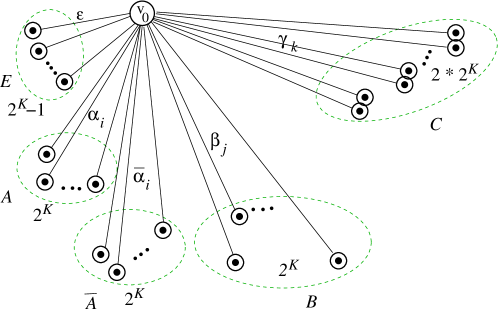
Figure 2: NP-hardness of Freeze-Tag for stars: In any good solution, a robot awakening one of the robots in set $C$ must have visited the sets $A$ and $B$ precisely once. This means that there is a cheap solution for this class of FTP instances, iff the elements of the sets $A$, $B$, $C$ can be grouped such that $\alpha_{i_{h}}+\beta_{j_{h}}+\gamma_{k_{h}}=d$.

We claim that there is a schedule to awaken all robots within time $L$, if and only if there is a feasible solution to the N3DM instance.

It is straightforward to see that the “if” part holds: Let $S_{1},S_{2},...,S_{n}$ be a feasible solution to the N3DM instance. Using a binary tree on the set $E$ (a “greedy cascade on $E$”), we can bring all $n$ robots in $E$ to the root at time $2\varepsilon K=2\varepsilon\log n$. These $n$ robots are sent to the $A$-leaves. Now there are $2n$ robots available, two each will get back to the root at time $a_{i}+2d$, $i=1,\ldots,n$. One of each pair is sent down the edge of length $\overline{\alpha_{i}}$, so that the whole set $\overline{A}$ gets awakened just in time $L$. The remaining $n$ robots (one for each $a_{i}$, call this robot $A_{i}$) get sent to wake up the robots of set $B$, such that $A_{i_{h}}$ is assigned to an edge of length $\beta_{j_{h}}$, if $a_{i_{h}}$ and $b_{j_{h}}$ belong to the same set $S_{h}$. This gets two robots for each $h$ (say, $A_{i_{h}}^{(1)}$ and $A_{i_{h}}^{(2)}$) back to the root at time $a_{i_{h}}+b_{j_{h}}+6d$. Send those two robots down the two edges of length $\gamma_{k_{h}}$. Because $a_{i_{h}}+b_{j_{h}}+c_{k_{h}}=d$, all robots in $C$ are awake at time $L$.

To see that a feasible schedule implies a feasible solution of the N3DM instance, first observe that no robot in $F=\overline{A}\cup C$ can wake up any other robot, as the corresponding edges are longer than $L/2$. Moreover, the same argument implies that no two robots in $F$ can be awakened by the same robot. Because the total number of robots is precisely $2|F|=6n$, we conclude that each robot in $E\cup A\cup B$ must wake up a different robot in $F$.

Clearly, no robot in $B$ can wake up a robot in $\overline{A}$ by the deadline $L$. Thus, the robots in $\overline{A}$ are awakened by a set of $n$ robots $\tilde{A}\subset E\cup A$. Notice that a robot in $\tilde{A}$ can neither visit a $B$-leaf nor two $A$-leaves and still meet the deadline.

The $2n$ robots in $C$ must be awakened by the $2n$ robots in $B\cup(E\cup A)\setminus\tilde{A}$. Because none of them has enough time to visit two $B$-leaves, each must visit exactly one $B$-leaf and then, by Lemma 4, travel immediately to a $C$-leaf. We can assume without loss of generality (by a simple exchange argument) that each pair of robots that has visited the same $B$-leaf is assigned to a pair of $C$-leaves at the same distance.

As explained above, each robot in $\tilde{A}$ can visit at most one $A$-leaf; the same is true for all robots in $(E\cup A)\setminus\tilde{A}$, because each must visit one $B$-leaf and one $C$-leaf afterwards. Because there are $2n$ robots in $E\cup A$ and also $2n$ visits to $A$-leafs, each robot in $E\cup A$ must visit exactly one $A$-leaf.

We next argue that, without loss of generality, a feasible solution uses a greedy cascade in the beginning to bring all $n$ robots in $E$ to the root at time $2\varepsilon K$. As described above, the greedy cascade guarantees that, later, each pair of robots returning from an $A$-leaf at distance $\alpha_{i}$ arrives at the center node at time $a_{i}+2d$. On the other hand, such a pair cannot arrive before time $2\alpha_{i}=a_{i}+2d-2\varepsilon K>a_{i}+2d-1$. Because the deadline $L$ as well as all remaining travel times to $\overline{A}$-leaves or $B$ and $C$-leaves are integral, the claim follows.

A simple exchange argument yields that, without loss of generality, the robots in $\overline{A}$ are awakened by the robots in $A$, i. e., $\tilde{A}=A$. Thus, each robot in $E$ travels to one $A$-leaf, then to a $B$-leaf and finally to a $C$-leaf. The time at which a robot in $E$ who has visited edges of length $\alpha_{i}$ and $\beta_{j}$ arrives at a $C$-leaf at distance $\gamma_{k}$ is $L-d+a_{i}+b_{j}+c_{k}$. Therefore, a schedule that awakens all robots by time $L$ implies a partition $S_{1},\dots,S_{n}$ with $a_{i_{h}}+b_{j_{h}}+c_{k_{h}}=d$ for all $h$. $\Box$

As the problem 3-Partition is strongly NP-complete, it is straightforward to convert the weighted stars in the construction into unweighted trees by replacing weighted edge by an unweighted path.

Corollary 10

The FTP is NP-hard, even for the special case of unweighted trees with one (asleep) robot at each leaf.

2.4 PTAS

We give a PTAS for the FTP on weighted stars with one awake robot at the central node, $v_{0}$, and an equal number $q$ of sleeping robots at each leaf. The underlying basic idea is to partition the set of edges into “short” and “long” edges. The lengths of the long edges are rounded such that only a constant number of different lengths remains. The approximate positions of the long edges in an optimal solution can then be determined by complete enumeration. Finally, the short edges are “filled in” by a variant of the greedy algorithm discussed in Subsection 2.2. During each step we may lose a factor of $1+O(\varepsilon)$, such that the resulting algorithm is a $(1+O(\varepsilon))$-approximation algorithm, so we get a polynomial-time approximation scheme.

Similar techniques have been applied for other classes of problems before, e.g., in the construction of approximation schemes for machine scheduling problems (see for example [24]). However, the new challenge for the problem at hand is to cope with the awakened robots at short edges whose number can increase geometrically over time.

Let $T\leq t^{*}$ be a lower bound on the makespan, $t^{*}$, of an optimal solution. For our purpose, we can set $T$ to $3/7$ times the makespan of the greedy solution, which can be determined in polynomial time. For a fixed constant $\varepsilon>0$, we partition the set of edges $E$ into two subsets

$$S := \{e\in E\mid\ell(e)\leq\varepsilon T\}\qquad\text{and}\qquad$$

$$L := \{e\in E\mid\ell(e)>\varepsilon T\}\enspace.$$

We call the edges in $S$ short and the edges in $L$ long. We modify the given instance by rounding up the length of each long edge to the nearest multiple of $\varepsilon^{2}T$.

Lemma 11

The optimal makespan of the rounded instance is at most $(1+O(\varepsilon))t^{*}$.

Proof: Consider the awakening tree corresponding to an optimal solution of the original instance. On any root-to-leaf path in the awakening tree, there can be at most $O(1/\varepsilon)$ long edges. (This is because $T\leq t^{*}\leq\frac{7}{3}T$, and long edges have length at least $\varepsilon T$.) In the rounding step we increase the length of a long edge by at most $\varepsilon^{2}T$. Therefore the length of any path, and thus the completion time of any robot in the solution given by the tree, is increased by at most $O(\varepsilon)\cdot T$. Because $T$ is bounded by $T\leq t^{*}\leq\frac{7}{3}T$, the claim follows. $\Box$

Any solution to the rounded instance with makespan $t$ induces a solution to the original instance with makespan at most $t$. Therefore, it suffices to construct a $(1+O(\varepsilon))$-approximate solution to the rounded instance. In the following we only work on the rounded instance and refer to it as instance $I$.

Lemma 12

There exists a $(1+\varepsilon^{2})$-approximate solution (which is possibly not a rational strategy) to instance $I$ that meets the requirement of Lemma 4, such that for each long edge the point in time that it is entered by a robot (its “start time”) is a multiple of $\varepsilon^{2}T$.

Proof: An optimal solution to instance $I$ can be modified to meet the requirement of the lemma as follows. Because the schedule obeys the structure from Lemma 4, any root-to-leaf path in the awakening tree first visits all short edges before all long edges. Whenever a robot wants to enter a long edge, it has to wait until the next multiple of $\varepsilon^{2}T$ in time. Because the lengths of long edges are multiples of $\varepsilon^{2}T$ all subsequent long edges are entered at times that are multiples of $\varepsilon^{2}T$. Therefore this modification increases the makespan of the solution by at most $\varepsilon^{2}T$. $\Box$

In the remainder of the proof we consider an optimal solution to instance $I$ meeting the requirements of Lemma 4 and Lemma 12. The makespan of this solution is denoted by $t^{*}$. Notice that both the number of different lengths of long edges and the number of possible start times are in $O(1/\varepsilon^{2})$. The positions of long edges in an optimal solution can be described by specifying for each possible start time and each edge length the number of edges of this length that are started at that time. Because each such number is bounded by the total number of edges $n$, there are at most $n^{O(1/\varepsilon^{4})}$ possibilities, which can be enumerated in polynomial time.

This enumerative argument allows us to assume that we have guessed the correct positions of all long edges in an optimal solution. Again, we can assume by Lemma 4 that any root-to-leaf path in the awakening tree first visits all short edges before all long edges. Therefore, the long edges are grouped together in subtrees. We must fill in the short edges near the root to connect the root of the awakening trees to the subtrees consisting of long edges. Given the start times $S(e)$ of the long edges $e\in L$, we group them into subtrees as follows. One by one, in order of nondecreasing start times, we consider the long edges. If an edge $e$ has not been assigned to a subtree yet, we declare it the root of a new subtree. If there are long edges $e^{\prime}$ with $S(e^{\prime})=S(e)+2\ell(e)$ that have not been assigned to a subtree yet, we assign at most $q+1$ of them as children to the edge $e$.

Let $p$ be the number of resulting subtrees and denote the start times of the root edges by $S_{1},\ldots,S_{p}$, indexed in nondecreasing order. Notice that, although the partition of long edges into subtrees is in general not uniquely determined by the vector of start times $(S(e))_{e\in L}$, the number of subtrees $p$ and the start times $S_{1},\ldots,S_{p}$ are uniquely determined.

It remains to fill in all short edges. This can be done by the following variant of the greedy algorithm: We set $S_{p+1}:=\infty$ and $i:=1$ in the beginning. Assume that a robot, coming from a short edge, gets to the central node at time $t$.

• If $t\geq S_{i}+2\varepsilon T$, then send the robot into the $i$th subtree and set $i:=i+1$.

• Else, if there are still short edges to be visited, then send the robot down the shortest of those edges.

• Else, if $i\leq p$, then send the robot into the $i$th subtree and set $i:=i+1$.

• Else stop.

Lemma 13

The above generalized greedy procedure yields a feasible solution to instance $I$ whose makespan is at most $t^{*}+4\varepsilon T\leq(1+4\varepsilon)t^{*}$.

Proof: We first argue that the solution computed by the generalized greedy procedure is feasible, i. e., all robots are awakened. We thus have to show the following: When a robot is sent into the $i$th subtree then either all short edges have been visited or there is at least one other robot traveling along a short edge (which will take care of the remaining subtrees and/or short edges).

Assume by contradiction that this condition is violated for some $i\in\{1,\dots,p\}$. Let $t$ denote the point in time when the generalized greedy procedure sends the last robot traveling on short edges into the $i$th subtree. We consider a (partial) solution to a modified instance $I^{\prime}$ which is obtained by replacing the first $i-1$ subtrees in the solution computed by the generalized greedy procedure until time $t$ by subtrees consisting of new short edges. These new edges and subtrees are chosen such that the resulting solution until time $t$ has the Shortest-Edge-First property, i.e., it is a (partial) greedy solution.

To be more precise, the construction of the modified instance $I^{\prime}$ and solution can be done as follows: Whenever the generalized greedy procedure sends a robot into one of the first $i-1$ subtrees, we replace the first edge of this subtree in the solution to the modified instance $I^{\prime}$ by a new edge whose length equals the length of the shortest currently available edge. Moreover, whenever a robot belonging to the modified subtree arrives at the center node before time $t$, we add a new short edge to the modified instance $I^{\prime}$ whose length equals the length of the shortest currently available edge and assign the robot to it.

Let $k$ be the number of awake robots in this greedy solution for the modified instance $I^{\prime}$ at time $t$. Notice that all $k$ robots belong to one of the modified subtrees.

The optimal solution to instance $I$ until time $t^{\prime}:=t-2\varepsilon T$ induces a solution $\sigma$ to the modified instance $I^{\prime}$ until time $t^{\prime}$ by again replacing the first $i-1$ subtrees of long edges by the corresponding subtrees of short edges.

We claim that there are at least $k+1$ awake robots in $\sigma$ at time $t^{\prime}$. Notice that the first $i-1$ subtrees are started at least $2\varepsilon T$ time units earlier than in the greedy solution (by construction of the generalized greedy procedure). Thus, the number of awake robots in these subtrees at time $t^{\prime}$ is at least $k$. Moreover, because the optimal solution awakens all robots, there must be at least one additional awake robot at time $t^{\prime}$ (taking care of the remaining edges).

However, in order to get $k+1$ awake robots, $\lceil k/q\rceil$ leaves must have been visited. Consider the $\lceil k/q\rceil$ shortest edges of the modified instance $I^{\prime}$. It follows from the discussion in the last paragraph that it takes at most $t^{\prime}$ time units to visit all of these edges. On the other hand, the makespan of the greedy solution is larger than $t$ because the number of awake robots in the greedy solution at time $t$ is only $k$. Because we only consider short edges of length at most $\varepsilon T$ and because $t-t^{\prime}=2\varepsilon T$, this is a contradiction to Corollary 8.

So far we have shown that the solution computed by the generalized greedy procedure visits all leaves. It remains to show that its makespan is at most $t^{*}+4\varepsilon T$.

Notice that the length of the time interval between two visits of a robot traveling on short edges to the central node is at most $2\varepsilon T$. Therefore, a robot is sent into the $i$th subtree before time $S_{i}+4\varepsilon T$, for $i=1,\dots,p$. As a consequence, the robots at each long edge are awake before time $t^{*}+4\varepsilon T$.

Finally, the same argument as in the feasibility proof above shows that all robots at short edges are awake at time $t:=t^{*}+2\varepsilon T$. This completes the proof. $\Box$

We summarize:

Theorem 14

There exists a polynomial-time approximation scheme for the FTP on (weighted) stars with the same number of robots at each leaf.

2.5 Any Number of Robots at Each Leaf

We give a constant-factor approximation algorithm for the FTP on general stars (centroid metric), where edge lengths may vary and leaves may have different numbers of asleep robots. Interestingly, we obtain this $O(1)$-approximation algorithm by merging (interleaving) two natural algorithms, each of which may perform poorly:

• The Shortest Edge First (SEF) strategy, where an awake robot at $v_{0}$ considers the set of shortest edges leading to asleep robots, and chooses one with a maximum number of asleep robots.

• The Repeated Doubling (RD) strategy, where the edge lengths traversed repeatedly (roughly) double in size, and in each length class, edges are selected by decreasing number of asleep robots. (A formal definition of the RD strategy is given later.)

Each of these algorithms is only a $\Theta(\log n)$-approximation, but their combination leads to an $O(1)$-approximation.

We first consider the Shortest-Edge-First strategy.

Lemma 15

The SEF strategy leads to a $\Theta(\log n)$-approximation.

Proof: Consider a tree having one edge of length $1+\varepsilon$ that leads to a leaf with $n-1$ robots, and $n-1$ edges, each of length $1$, with one robot at each of the leaves; see Figure 3. The Shortest-Edge-First strategy has makespan $\Theta(\log n)$, whereas an optimal strategy has makespan $O(1)$. Thus, SEF is an $\Omega(\log n)$ approximation algorithm. By Proposition 2, any rational strategy is an $O({\log n})$ approximation algorithm. $\Box$

Figure 3: Example in which Shortest-Edge-First yields a solution of makespan $\Theta(\log n)$, while the optimal is $O(1)$.

Next we consider the Repeated Doubling strategy. A robot at $v_{0}$ faces the following dilemma: should the robot choose a short edge leading to a small number of robots (which can be awakened quickly) or a long edge leading to many robots (but which takes longer to awaken)? There are examples that justify both decisions, and where a wrong decision can be catastrophic. See Figure 4.

We begin our analysis by assuming that all branches have lengths that are powers of $2$. This assumption is justified because we can take an arbitrary problem and stretch all the edges by at most a factor of $2$. Now any optimal solution for the original problem becomes a solution to this stretched problem, in which the makespan is increased by at most a factor of $2$. Thus, a $k$-approximation to the stretched problem is a $2k$-approximation to the original problem.

Thus, we have reduced the problem on general stars to the problem on stars whose edge lengths are powers of $2$. We partition the edges into length classes. Within each length class, it is clear which edge is the most desirable to awaken: the one housing the most robots. However, how can we choose which length class the robot should visit first? Suppose that an optimal algorithm chooses an edge of length $2^{j}$ at some point in time. We can visit edges of lengths $1,2,4,8,\ldots,2^{j}$ and only increase the makespan by a factor of $3$. That is, we use repeated doubling to “hedge our bets” about what is the best path to take next. However, if the right choice to make is to awaken robots in a nearby length class, then we may suffer by sending robots on a repeated-doubling trajectory to long edges.

In summary, the Repeated Doubling (RD) algorithm is as follows. When a robot wakes up, it awakens the most desirable edge in length class $1,2,4,8,\ldots$. When the robot runs out of length classes, it starts the repeated doubling process anew.

The Repeated Doubling strategy may have poor performance:

Lemma 16

The RD strategy yields an $\Theta(\log n)$-approximation.

Proof: Consider a star having $n/2$ edges of length $1$ and $n/2$ edges of length $\log n$, with a single robot at each leaf. Refer to Figure 4. The optimal solution has makespan $\Theta({\log n})$ — first the robots awaken all the short branches (in time $\Theta({\log n})$), and then $n/2$ robots awaken the long branches (again in time $\Theta(\log n)$). The RD strategy, on the other hand, has makespan $\Theta(\log^{2}n)$. Thus, the RD strategy is an $\Omega(\log n)$ approximation. By Proposition 2, any rational strategy is an $O({\log n})$ approximation algorithm, establishing our bound. $\Box$

Figure 4: Example in which Repeated Doubling yields a solution of $\Theta(\log^{2}n)$, while the optimum is $O(\log n)$.

We now merge these two previous strategies to obtain what we call the Tag-Team Algorithm: When a robot is first awakened, it awakens one edge in each length class $1,2,4,8,\ldots$. Before each doubling step, the robot awakens the shortest edge that it can find. When the robot runs out of length classes, it starts the repeated doubling process anew. Naturally, the robot skips any length class no longer containing edges.

Theorem 17

The Tag-Team algorithm gives a 14-approximation for the FTP on centroid metrics (general stars).

Proof: We begin by restricting ourselves to the special case in which all edge lengths are powers of 2; because any general instance can be transformed to this special case, while at most doubling the edge lengths, this restriction results in at most doubling the cost of a solution.

Consider an optimal solution given by a wake-up tree ${\cal T}^{*}$. We can assume without loss of generality that an edge is awakened before all other edges in the same length class with a smaller number of robots. Moreover, if there are several edges with the same number of robots in a length class, we break ties and assume that the Tag-Team algorithm visits these edges in the same order as the optimal solution does.

We show by induction that if in the optimal awakening tree ${\cal T}^{*}$ an edge $e$ is awakened at time $t$, then the Tag-Team algorithm awakens this edge $e$ at or before time $7t$.

Suppose that in the optimal awakening tree ${\cal T}^{*}$ at time $t$ a robot ${r}$ awakens the robots ${r_{1}},{r_{2}},\ldots,{r_{k}}$ at the end of an edge $e$, where $e$ has length $\ell(e)$. Consider the next edge that each of the robots ${r_{1}},{r_{2}},\ldots,{r_{k}}$ awakens in the optimal awakening tree ${\cal T}^{*}$. Specifically, suppose that in ${\cal T}^{*}$, robot ${r_{i}}$ travels to an edge $e_{i}$ of length ${\ell(e_{i})}$. That is, in ${\cal T}^{*}$ at time $t+\ell(e)+\ell(e_{i})$, robot $r_{i}$ awakens the robots at the end of edge $e_{i}$.

Now we consider when these robots are awakened in the Tag-Team algorithm. By induction, suppose that robot $r$ was awakened at or before time $7t$. In the tag-team algorithm each of the awakened robots ${r_{1}},{r_{2}},\ldots,{r_{k}}$ performs a repeated doubling trajectory, ultimately awakening the edge in the appropriate length class. The worst case is when the edge taken in the SEF branches has the same length as the edge taken in the RD branches. Thus, two edges of length $2^{j}$ are traversed (for $j=1,2,\ldots$), one during a RD step and one during an SEF step, and each edge is traversed in both directions. Therefore, either $r_{i}$ awakens $e_{i}$ by time

$$7t+\ell(e)+2\cdot 2\cdot(1+2+4+\dots+\ell(e_{i})/2)+2\ell(e_{i})+\ell(e_{i})\,\leq\,7t+\ell(e)+7\ell(e_{i})\,,$$

or edge $e^{\prime}_{i}$ was already awakened. That is, even without knowing the edge class where $r_{i}$ should go directly, it gets there eventually. But what about the original robot $r$, which continues its repeated doubling trajectory to larger edges when in ${\cal T}^{*}$ robot $r$ visits a smaller edge? Robot $r$ plays tag-team awakening at least one robot on the smallest edge possible, and this new robot performs $r$’s duties. Thus, this robot in time $\leq 7t+\ell(e)+7\ell(e_{i})$ awakens the edge class that $r$ would awaken in ${\cal T}^{*}$. $\Box$

At this point it is still open how this approximation factor can be improved. In fact, we conjecture that there is a $(1+\varepsilon)$-approximation:

Conjecture 18

There is a PTAS for the freeze-tag problem on weighted stars with not necessarily the same number of robots at each leaf.

3 General Graphs

Now we discuss the FTP on general graphs $G=(V,E)$ with nonnegative edge weights $\ell(e)$. We let $\delta(v)$ denote the degree of $v$ in $G$.

3.1 A Competitive Online Algorithm

As Theorem 9 illustrates, even the presence of a single vertex $v$ with a high degree causes the problem to be NP-hard, showing that the resulting choices may be difficult to resolve. This makes it plausible that the complete absence of high-degree nodes could make the problem more tractable. As we will see later on, this is not the case: Even for graphs of maximum degree 5, finding a solution within 5/3 of the optimum is NP-hard.

However, it is not hard to see that a sufficient number, $r(v_{i})$, of robots at each vertex $v_{i}$ yields an easy problem:

Lemma 19

Suppose $r(v_{0})\geq\delta(v_{0})$ for the source node $v_{0}$, and $r(v_{i})\geq\delta(v_{i})-2$ at any other node $v_{i}$ in $G$. Then the FTP can be solved by breadth-first search.

This observation is based on the simple fact that any node in a breadth-first search (BFS) tree has minimal possible distance from the root, making the depth of this tree a general lower bound on the makespan of a wake-up tree. If $r(v_{0})\geq\delta(v_{0})$ and $r(v_{i})\geq\delta(v_{i})-2$ for any $v_{i}\neq v_{0}$, we have sufficiently many robots available to use a BFS tree as the wake-up tree, and the claim follows.

As we noted in the introduction, the online version of the FTP is of interest in some potential applications. Using the fact that BFS uses only local information, we obtain some simple online results for the FTP, as we now describe. We let

$$\Delta_{G}:=\max\{\frac{\delta(v_{0})}{r(v_{0})},\frac{\delta(v_{i})-2}{r(v_{i})},i=1,\ldots,n-1\}.$$

For an edge-weighted graph $G$ and any node $v$ of $G$, we let $\rho_{v}$ denote the maximum ratio of weights for two edges incident on $v$; i.e., $\rho_{v}\geq 1$ is the ratio of the maximum edge weight among edges incident on $v$ to the minimum edge weight among edges incident on $v$. We say that $G$ has locally bounded edge weights if there exists a constant, $C$, such that $\rho_{v}\leq C$ for all $v$ in $G$.

Theorem 20

Let $G$ be an edge-weighted graph with locally bounded edge weights. Then, there is a linear-time online algorithm for the FTP on $G$ that guarantees a competitive ratio of $O(\log\Delta_{G})$.

Proof: The idea is to simulate a breadth-first search at each node: At any vertex $v_{i}$, use the robots at $v_{i}$ to awaken all robots at neighboring nodes prior to sending robots to awaken robots at nodes that neighbor the neighboring nodes of $v_{i}$. This is readily achieved with a binary wakeup tree of unweighted depth $O(\log\frac{\delta(v_{0})}{r(v_{0})})$ for the root $v_{0}$, and $O(\log\frac{\delta(v_{i})-2}{r(v_{i})})$ for any other vertex $v_{i}$, as the vertex used to enter $v_{i}$ does not need to be awakened. Thus, with the assumption of locally bounded edge weights, the time needed to do this awakening is $O(\log\frac{\delta(v_{0})}{r(v_{0})})$ (or $O(\log\frac{\delta(v_{i})-2}{r(v_{i})})$) times the weight of a minimum-weight edge incident on $v_{0}$ (or $v_{i}$). Thus, each robot is awakened by time $O(\log\Delta_{G})$ times the length of the minimum-weight path from the root to the node where the robot originally sleeps. This implies the claim. $\Box$

There is an $\Omega(\log\Delta)$ lower bound on the competitive ratio of any online algorithm, as the following example shows. Specifically, $v_{0}$ has $k$ neighbors, each at distance one from $v_{0}$ and each having exactly one sleeping robot. One of these neighbors of $v_{0}$ has adjacent to it a tree with diameter $\varepsilon$, having a population of at least $k$ sleeping robots. An online algorithm has no knowledge of which neighbor of $v_{0}$ has the adjacent tree of many sleeping robots; an adversary can make this neighbor be the last one awakened by the algorithm. An optimal offline strategy awakens this neighbor first, then awakens the neighboring tree of many robots, which then return to $v_{0}$ and awaken the rest of $v_{0}$’s neighbors, in total time $O(1)$. The online strategy takes time $\Omega(\log\Delta)$.

3.2 Hardness of Approximation

As it turns out, there is no realistic hope for a PTAS on general graphs of bounded degree, even if we go beyond strictly local, i.e., online procedures:

Theorem 21

It is NP-hard to approximate the FTP on general weighted graphs within a factor less than 5/3, even for the case of $\Delta_{G}=4$ and one robot at each node.

Proof: The reduction is from 3SAT. Without loss of generality, we assume that we have $n=2^{K}$ variables. For technical reasons, we add $n$ clauses of size 2 of the form “$x$ or not $x$”, one for each variable.

This instance will be mapped to an FTP instance on a weighted graph of bounded degree with one robot per vertex, such that we have a solution of makespan $3/2+O(\varepsilon\log n)$ if there is a satisfying truth assignment, and a makespan of at least 5/2 if there is no such truth assignment. By choosing $\varepsilon=o(\log n)$, this implies that approximating the resulting class of FTP instances within a factor of less than 5/3 requires finding a satisfying truth assignment, hence the claim.

Figure 5: NP-hardness of 5/3-approximation of Freeze Tag in general graphs.

We now give details of the construction. See Figure 5. From the root, build a binary tree of depth $\varepsilon\log(n/2)$, resulting in two awake robots at each of the $n/2$ preliminary leaves, after time $\varepsilon\log(n/2)$.

Next group the $n$ variables in an arbitrary way to $n/2$ pairs, and assign a pair to each preliminary leaf. Each pair of variables is represented by four more vertices, two corresponding to “true”, two corresponding to “false”. All get connected to the respective preliminary leaf, using an edge of “intermediate” length 1/2. The two vertices for the same variable get connected to each other, using an edge of “long” length 1.

If $c(x)$ is the number of clauses in which some literal $x$ occurs, attach a small binary tree of height $O(\varepsilon)$ to allow $c(x)+1$ awake robots at cost $O(\varepsilon)$ when the literal node is reached. (This does not affect the overall $\Delta$.)

Finally, add one vertex per clause (including the artificial ones stated above.) Using an edge of length 1, connect each literal vertex to the vertices representing the clauses in which the literal occurs.

Now a truth assignment induces a wake-up tree of makespan $3/2+O(\varepsilon\log n)$. After going through the initial binary tree, we have $n$ awake robots at the preliminary leaves. For each variable, pick the node corresponding to the literal in the given truth assignment. Use $c(x)$ of the robots close to this literal to wake up all corresponding clause nodes, and the remaining robot to wake up the counterpart $\overline{x}$ of $x$.

Conversely, consider a solution of makespan $3/2+O(\varepsilon\log n)$, and a wakeup path from the root to a robot at a clause vertex. Clearly, such a path must contain at least one long edge of length 1, and an odd number of edges of intermediate length 1/2. Assume that all such paths contain precisely one edge of length 1, and one of length 1/2. Consider all the auxiliary clauses of type $(x_{i}\vee\overline{x_{i}})$ and their wakeup paths from the root. There are $n$ of these paths, and $n$ robots within distance $O(\varepsilon\log n)$ from the root. By the time $1/2+O(\varepsilon\log n)$, for each auxiliary clause, one awake robot must be within distance $1+O(\varepsilon\log n)$. This means that at time $1/2+O(\varepsilon\log n)$, for each of the $n$ variables precisely one of the $n$ robots close to the root must have moved to either vertex $x_{i}$ or to vertex $\overline{x_{i}}$, but not both. This means that the path of robots induces a truth assignment for the variable. Furthermore, at time $1/2+O(\varepsilon\log n)$ there must be one awake robot within distance 1 of each clause vertex; therefore, all clauses are satisfied by the induced truth assignment.

This means that there cannot be a solution of makespan $3/2+O(\varepsilon\log n)$, if there is no satisfying truth assignment. Furthermore, if there is no solution with only one short and one intermediate edge on each wakeup path to a clause vertex, any such path in an optimal solution must have at least two long edges and one intermediate edge, or at least one long edge and three intermediate edges. This means that if there is no satisfying truth assignment, an optimal solution must have makespan at least $5/2+\Omega(\varepsilon\log n)$.

This concludes the proof. $\Box$

4 Freeze-Tag in Geometric Spaces

We now assume that the domain ${\cal D}=\Re^{d}$ and that the distance, $d(p_{i},p_{j})$, between the points $p_{i},p_{j}\in P$ is the Euclidean distance (or any $L_{p}$ metric). In this section, we begin by showing a constant-factor approximation. We then introduce the notion of “pseudo-balanced” awakening trees. Finally, we show how these two ideas are combined to yield an efficient PTAS for the geometric Freeze-Tag Problem.

4.1 Constant-Factor Approximation Algorithm

Theorem 22

There is an $O(1)$-approximation algorithm, with running time $O(n\log n)$, for the geometric FTP in any fixed dimension $d$. The algorithm yields a wake-up schedule with makespan $O(diam(R))$, where $diam(R)$ denotes the diameter of the point set $R$.

Proof: For each of the points $v\in R$, we consider $K$ sectors defined by rays emanating from the points at angles $0,2\pi/K,2(2\pi/K),3(2\pi/K),\ldots$. Let $u_{j}(v)$ denote the point (if any) of $R$ in the $j$th sector that is closest to $v$; if there are no points of $R$ in the $j$th sector of $v$, then $u_{j}(v)$ is undefined. We can compute the $u_{j}(v)$ points, for all $j$ and all $v\in R$, in total time $O(Kn\log n)$, using standard Voronoi diagram-based methods [13].

We sort the points $u_{j}(v)$ by distance from $v$; let these points be $u_{1},u_{2},\ldots,u_{K^{\prime}}$, in sorted order by distance from $v$. The wake-up strategy we employ is as follows: Once the robot at $v$ is unfrozen, it follows the path $v,u_{1},u_{2},\ldots,u_{K^{\prime}}$, awakening the nearest robot in each of the $K^{\prime}\leq K$ nonempty sectors about it. (Of course, some of these robots may have already been awakened before it gets to their (initial) positions. This potentially saves it the effort of going to all of these nearby neighbors, allowing for some possible further improvement in our constant factor.)

We now analyze the performance of this algorithm. Let $G_{K}=(R,E_{K})$ be the graph that links each point $v$ to the points $u_{j}$ that are its nearest neighbors in the $K$ sectors about $v$. Such a graph $G_{K}$ is known as a $\Theta$-graph, for $\Theta=2\pi/K$, and is known to be a $t$-spanner for values of $K\geq 9$ (e.g., see [16]). This means that distances in the graph $G_{K}$ approximate to within a constant factor the Euclidean lengths of the edges in the complete graph $G$ on $R$.

Assume that the robot at point $v_{\ell}$ is the last one to be unfrozen by our algorithm. What is the path length of the “signal” (the unfreezing tag) in getting from $v_{0}$ to $v_{\ell}$? We know that if some point $v$ is reached by the signal by distance $t$, then any neighbor, $u_{j}(v)$, of $v$ in the graph $G_{K}$ is reached by distance $\leq t+\xi$, where $\xi$ is the length of the path $v,u_{1},u_{2},\ldots,u_{j}$; thus, $\xi\leq(2j-1)\cdot d(v,u_{j})\leq(2K-1)\cdot d(v,u_{j})$. Thus, the signal will reach $v_{\ell}$ within a distance of at most $(2K-1)$ times the distance from $v_{0}$ to $v_{\ell}$ in $G_{K}$. For constant $K\geq 9$, distances in $G_{K}$ approximate distances in the Euclidean plane, up to a constant depending on $K$. This implies that the signal gets to $v_{\ell}$ within distance $O(d(v_{0},v_{\ell}))$; because $d(s,p_{\ell})$ is a lower bound on the optimal makespan, $t^{*}$, we have shown that we have an $O(1)$-approximation. $\Box$

Figure 6: An $O(1)$-approximation algorithm for the geometric FTP in any fixed dimension $d$. The algorithm generates a wake-up schedule with makespan $O(diam(R))$. When a robot at point $p$ first awakens, it awakens the nearest asleep robot in each of $K$ sectors, in order of increasing distance from the point $p$.

4.2 Pseudo-Balanced Awakening Trees

We show how to transform an arbitrary awakening tree ${\cal T}$ into an awakening tree ${\cal T}_{b}$ whose makespan is only marginally longer, and where no root-to-leaf path travels through too many edges. This transformation is critical for the PTAS that follows in the next subsection.

We say that a wake-up tree is pseudo-balanced if each root-to-leaf path in the tree has $O(\log^{2}n)$ nodes. We have the following theorem:

Theorem 23

Suppose there exists an awakening tree, ${\cal T}$, having makespan $t$. Then, for any $\mu>0$, there exists a pseudo-balanced awakening tree, ${\cal T}_{b}$, of makespan $t_{b}\leq(1+\mu)t$.

Proof: First we perform a heavy-path decomposition (e.g., see [36]) of the tree ${\cal T}$. For each node $v$, let $d(v)$ be the number of descendents. Consider a node $u$ with children $v_{1},\ldots,v_{k}$. The edge $(u,v_{i})$ is heavy if $v_{i}$ has more descendents than any other child of $u$; i.e., $i=\arg\max_{j}d(v_{j})$. If $(u,v_{j})$ is a light (non-heavy) edge, then at most half of $u$’s descendents are $v_{j}$’s descendents; that is, $d(v_{j})\leq d(u)/2$. Thus, in any root-to-leaf path in ${\cal T}$ there are at most $\log n$ light edges. Also, heavy edges form a collection of disjoint paths (because there is one heavy edge from a node to one of its children). We say that a heavy path $\pi^{\prime}$ is a child of heavy path $\pi$ if one end node of $\pi^{\prime}$ is the child of a node in $\pi$. The heavy-path decomposition forms a balanced tree of heavy paths, because any root-to-leaf walk in ${\cal T}$ visits at most $\log n$ light edges, and therefore at most $\log n$ heavy paths.

Figure 7: The awakening tree is partitioned into heavy paths, each of which is partitioned into subpaths of length $\xi$.

We use these heavy paths to refine the description of the wake-up tree. See Figure 7. We can assume that in $T$ each heavy path is awakened by one robot, the robot that awakens the head of the heavy path (node closest to $v_{0}$) and that no robot awakens more than one heavy path. In this way, a heavy-path decomposition of ${\cal T}$ corresponds to an awakening schedule with one robot per path.

Because ${\cal T}$ has makespan $t$, each heavy path has length at most $t$. We divide the heavy path into subpaths of length $\xi=\mu t/(2\log n)$. Note that on any root-to-leaf path in ${\cal T}$, we visit at most $O((1+1/\mu)\log n)$ different subpaths. In the original wake-up tree, all nodes in one length $\xi$ subpath are awakened by a single robot. Thus, by construction, a robot $\delta$ units from the beginning of the subpath is awakened $\delta$ units after the beginning (head) of the subpath. In our modified solution, the robots in a length $\xi$ subpath share in the collective awakening of all the robots in the subpath.

We guarantee that we can begin awakening one subpath $\xi$ time units after we began awakening the previous subpath. We further guarantee that all of the robots are awake and back in their original asleep positions by $2\xi$ time units after the first robot in the subpath is originally awakened. Thus, a robot $\delta$ units from the beginning of the subpath is only guaranteed to be awake $2\xi$ units after the robot at the beginning of the subpath is awakened, which could entail a total delay of $2\xi$ over the original awakening.

Figure 8: Robot $r_{1}$ awakens the subproblem $(r_{1},r_{3})$ by first awakening $r_{2}$, the last robot (if any) before distance $\xi/3$. Robot $r_{2}$ is then in charge of awakening $(r_{1},r_{2})$ before returning to its original position. Robot $r_{1}$ then awakens $(r_{2},r_{3})$.

We awaken a subpath as follows; see Figure 8. We consider the subpath to be oriented from “left” (the head, closest to source $v_{0}$) to “right”. The first robot $r_{1}$, at the left end of the subpath, travels along the subpath until the last (asleep) robot, $r_{2}$, before position $\xi/3$, if such a robot $r_{2}$ exists. If robot $r_{2}$ exists, then $r_{2}$ is sent leftwards with the responsibility to awaken all asleep robots in the interval $(r_{1},r_{2})$, and this subproblem is solved recursively; thus, $r_{2}$ is responsible for initiating the awakening of all robots in the interval $(r_{1},r_{2})$, and all robots must return to their initial positions. If no robot $r_{2}$ is encountered by $r_{1}$ before position $\xi/3$, then we use $r_{1}$ to solve recursively the subproblem $(\xi/3,\xi)$.

We continue the strategy until a subproblem’s length drops below $\xi/\log n$ and then resort to a different wake-up strategy. The responsible robot, $r$, goes to the median robot of the subproblem and awakens it, and continues in its same direction. The robot it just awakened goes in the opposite direction and recursively does the same thing, heading for the median in its subproblem, etc. Because a segment has at most $n$ robots in it, this strategy takes time at most $\log n\cdot\xi/\log n$.

Consider a heavy path composed of subpaths of length $\xi$. Consider any robot at position $\delta$ along the heavy path. The original wake-up tree will awaken this robot $\delta$ units after the first robot of the heavy path. The new solution may awaken this robot as much as $\delta+2\xi$ time units after the first robot of the heavy path; one additive delay of $\xi$ is from the first phase of the awakening and the second additive delay of $\xi$ is from the second phase of the awakening.

Because there are at most $\log n$ heavy paths on any root-to-leaf walk and there is an accumulated delay of at most $2\xi$ per heavy path, the total delay on any root-to-leaf path is at most $2\xi\log n$. Because $\xi=\mu t/\,2\log n$, the accumulated delay in the makespan is at most $\mu t$.

On any root-to-leaf path in ${\cal T}$ there are at most $O(\log n)$ subpaths. Each of these subpaths in our new wake-up tree is transformed into a wake-up subtree of height $O(\log n)$. Thus, on any root-to-leaf path in the new wake-up tree there are at most $O(\log^{2}n)$ nodes, and therefore our wake-up tree is pseudo-balanced. $\Box$

4.3 PTAS

We give a $(1+\varepsilon)$-approximation algorithm (PTAS) for the Euclidean (or $L_{p}$) Freeze-Tag Problem in any fixed dimension. Our algorithm runs in nearly linear time, $O(2^{poly(1/\varepsilon)}+n\log n)$. It is important to note that the exponential dependence on $1/\varepsilon$ appears additively in our time bound, not multiplying $n\log n$.

Figure 9: PTAS for geometric instances. Rescale so that all robots lie in a unit square. Look at $m$-by-$m$ grid of pixels, where $m=O(1/\varepsilon)$. Consider an enumeration over a special class of wake-up trees on a set $P$ of representative points, one per occupied pixel.

We divide the plane into a constant number of square tiles or pixels. Specifically, we rescale the coordinates of the $n$ input points (robots), $R$, so that they lie in the unit square, and we subdivide the square into an $m$-by-$m$ grid of pixels, each of side length $1/m$. (We will select $m$ to be $O(1/\varepsilon)$.) We say that a pixel is empty if it contains no robots.

Our algorithm is based on approximately optimizing over a restricted set of solutions, namely those for which all of the robots within a pixel are awakened before any robot leaves that pixel. Note that by Theorem 22, once one robot in a pixel has been awakened, all of the robots in the pixel can be awakened within additional time $O(1/m)$, because this is the diameter of the pixel.

We now describe the algorithm. We select an arbitrary representative point in each nonempty pixel. We pretend that all robots in the pixel are at this point, and we enumerate over all possible wake-up trees on the set, $P$, of representative points. (If there are $r$ robots in a given pixel, then we only enumerate wake-up trees whose corresponding out-degree at that pixel is at most $\min\{m^{2}-1,r+1\}$.) Because there are only a constant number of such trees (at most $2^{O(m^{2}\log m)}$, because $|P|\leq m^{2}$), this operation takes time $2^{O(m^{2}\log m)}$, which is a constant independent of $n$. Recall that a wake-up tree is pseudo-balanced if each root-to-leaf path in the tree has $O(\log^{2}m)$ nodes. Among those wake-up trees for $P$ that are pseudo-balanced, we select one, ${\cal T}_{b}^{*}(P)$, of minimum makespan, $t_{b}^{*}(P)$. We convert ${\cal T}_{b}^{*}(P)$ into a wake-up tree for all of the input points $R$ by replacing each $p\in P$ with an $O(1)$-approximate wake-up tree for points of $R$ within $p$’s pixel, according to Theorem 22. This step takes total time $O(n\log n)$. The total running time of the algorithm is therefore $O(2^{O(m^{2}\log m)}+n\log n)$. Correctness is established in the following lemmas.

Lemma 24

There is a choice of representative points $P$ such that the makespan of an optimal wake-up tree of $P$ is at most $t^{*}(R)$.

Proof: For each pixel, we select the representative point to be the location of the first robot that is awakened in an optimal solution, ${\cal T}^{*}(R)$, for the set of all robots. Then, for this choice of $P$, the spanning subtree of $P$ within ${\cal T}^{*}(R)$ defines a feasible wake-up tree for $P$ of makespan no greater than that of ${\cal T}^{*}(R)$ (namely, $t^{*}=t^{*}(R)$). $\Box$

Lemma 25

For any two choices, $P$ and $P^{\prime}$, of the set of representative points, we have $t_{b}^{*}(P)\leq t_{b}^{*}(P^{\prime})+O((\log^{2}m)/m)$.

Proof: Pixels have size $O(1/m)$ and there are at most $O(\log^{2}m)$ awakenings in each root-to-leaf path of a pseudo-balanced tree; thus, any additional wake-up cost is bounded by $O((\log^{2}m)/m)$. $\Box$

A similar proof yields:

Lemma 26

For any pseudo-balanced wake-up tree of $P$, there exists a wake-up tree, ${\cal T}(R)$, with makespan $t(R)\leq t_{b}(P)+O((\log^{2}m)/m)$.

In summary we have the following result:

Theorem 27

There is a PTAS, with running time $O(2^{O(m^{2}\log m)}+n\log n)$, for the geometric FTP in any fixed dimension $d$.

Proof: The time bound was already discussed. The approximation factor is computed as follows. By the lemmas above, the makespan, $t$, of the wake-up tree we compute obeys:

$$t \leq t_{b}^{*}(P)+O((\log^{2}m)/m)$$

$$\leq t_{b}^{*}(P^{\prime})+2\cdot O((\log^{2}m)/m)$$

$$\leq t_{b}(P^{\prime})+O((\log^{2}m)/m)$$

$$\leq (1+\mu)t^{*}+O((\log^{2}m)/m)$$

$$\leq t^{*}\left(1+\mu+\frac{C\log^{2}m}{m}\right)$$

$$\leq t^{*}(1+\varepsilon),$$

for appropriate choices of $\mu$ and $m$, depending on $\varepsilon$. (We also used the fact that $t^{*}\geq diam(R)\geq 1$.) $\Box$

At this point the complexity of the FTP for geometric distances in $\Re^{d}$ has been unsettled for several years. In fact, this issue is the topic of Problem #35 on the well-known list [14] known as “The Open Problems Project”. We have the following conjecture.

Conjecture 28

The freeze-tag problem is NP-hard for Euclidean or Manhattan distances in the plane.

5 Conclusion

We have introduced the Freeze-Tag Problem. We have given a number of algorithmic results for various scenarios. For the case of star graphs, we have shown NP-hardness, and analyzed approximation algorithms, in particular for the case of an identical number of robots at each leaf, for which we have given a simple 7/3 greedy algorithms, and a more complicated PTAS. We have also shown the existence of constant-factor approximation methods for general star scenarios, and a 5/3 bound on the approximation ratio in general weighted graphs, even for bounded degree and one robot at each node. Furthermore, we have studied the Freeze-Tag Problem in geometric spaces, where we showed the existence of constant-factor approximation algorithms, including a PTAS.

Obviously, there is a considerable number of open problems that deserve further study:

1. Is there a lower bound on the approximability of the Freeze-Tag Problem on tree metrics?

2. Is there an $o(\log n)$-approximation algorithm for the Freeze-Tag Problem in general weighted graphs?

3. Is the FTP in low-dimensional geometric spaces NP-hard?

4. Is there a PTAS for the FTP in trees with different numbers of robots at each leaf?

5. Is there an $o(\log n)$- (or, ideally, an $O(1)$-) approximation algorithm for the FTP for points in a polygon, where distances are measured according to the length of a shortest path in the polygon? Such an algorithm would apply also to the FTP in general trees.

6. Can our results be extended to the case of several sources?

7. In a geometric scenario, how does the problem change if a robot only has to get “close” to another robot (say, within distance 1) in order to unfreeze it?

It is also of interest to consider more game-theoretic aspects related to freeze tag, like considering algorithmic issues arising from the full game of freeze-tag in the presence of an adversary. This is somewhat related to the Competing Salesman Problem [17], where two salesmen travel in a graph and try to visit vertices before the opponent does.

As described in the introduction, there are many other related questions, and we do expect many more interesting results arising from this research.

Acknowledgments

We thank Doug Gage for discussions motivating this research. We are also grateful to Regina Estkowski, Tien-Ruey Hsiang, Nenad Jovanovic, David Payton, and Marcelo Sztainberg for many helpful discussions. We thank Asaf Levin for pointing out the lower bound in Section 4.1 and for alerting us to the omission of the assumption of locally bounded edge weights in Theorem 20 in the conference draft of this paper. We thank Gerhard Trippen and other anonymous referees for several useful comments that helped to improve the overall presentation of this paper.

Esther Arkin acknowledges support from HRL Laboratories, the National Science Foundation (CCR-0098172, CCF-0431030), and Sandia National Laboratories. Michael Bender acknowledges support from HRL Laboratories, the National Science Foundation (EIA-0112849), and Sandia National Laboratories. Work by Sándor Fekete was performed in part while visiting Stony Brook, with partial support by the DFG Focus Program 1126, “Algorithmic Aspects of Large and Complex Networks,” grant no. Fe 407/8-1. Joseph Mitchell acknowledges support from HRL Laboratories, Honda Fundamental Research Labs, Metron Aviation, NASA Ames Research Center (NAG2-1325, NAG2-1620), the National Science Foundation (CCR-0098172, ACI-0328930, CCF-0431030), and the US-Israel Binational Science Foundation (Grant 2000160). Martin Skutella is supported in part by the EU Thematic Network APPOL I+II, “Approximation and Online Algorithms,” IST-1999-14084 and IST-2001-30012, and by the DFG Focus Program 1126, “Algorithmic Aspects of Large and Complex Networks,” grant no. SK 58/4-1.

References

- [1] S. Albers and M. R. Henzinger. Exploring unknown environments. In Proceedings of the 29th Annual ACM Symposium on the Theory of Computing (STOC), pages 416–425, 1997.
- [2] S. Albers, K. Kursawe, and S. Schuierer. Exploring unknown environments with obstacles. In Proceedings of the 10th Annual ACM-SIAM Symposium on Discrete Algorithms (SODA), pages 842–843, 1999.
- [3] S. Alpern and S. Gal. The Theory of Search Games and Rendezvous. Kluwer Academic Publishing, 2002.
- [4] E. J. Anderson and S. P. Fekete. Two-dimensional rendezvous search. Operations Research, 49:107–118, 2001.
- [5] E. M. Arkin, M. A. Bender, S. P. Fekete, J. S. B. Mitchell, and M. Skutella. The Freeze-Tag Problem: How to wake up a swarm of robots. In Proceedings of the 13th ACM-SIAM Symposium on Discrete Algorithms (SODA), pages 568–577, 2002.
- [6] E. M. Arkin, M. A. Bender, D. Ge, S. He, and J. S. B. Mitchell. Improved approximation algorithms for the Freeze-Tag Problem. In Proceedings of the 15th Annual ACM Symposium on Parallelism in Algorithms and Architecture (SPAA), pages 295–303, 2003.
- [7] T. Balch. http://www.teambots.org.
- [8] A. Bar-Noy, S. Guha, J. Naor, and B. Schieber. Multicasting in heterogeneous networks. In Proceedings of the 30th Annual ACM Symposium on Theory of Computing (STOC), pages 448–453, 1998.
- [9] Y. Bartal. On approximating arbitrary metrics by tree metrics. In ACM Symposium on Theory of Computing (STOC), pages 161–168, 1998.
- [10] E. Bonabeau, M. Dorigo, and G. Theraulaz. Swarm Intelligence: From Natural to Artificial Systems. Oxford University Press, 1999.
- [11] A. M. Bruckstein, C. L. Mallows, and I. A. Wagner. Probabilistic pursuits on the grid. American Mathematical Monthly, 104(4):323–343, 1997.
- [12] M. Charikar, C. Chekuri, A. Goel, S. Guha, and S. Plotkin. Approximating a finite metric by a small number of tree metrics. In Proceedings of the 39th Annual IEEE Symposium on Foundations of Computer Science (FOCS), pages 379–388, 1998.
- [13] K. L. Clarkson. Approximation algorithms for shortest path motion planning. In Proceedings of the 19th Annual ACM Symposium on the Theory of Computing (STOC), pages 56–65, 1987.
- [14] E. D. Demaine, J. S. B. Mitchell, and J. O’Rourke. The Open Problems Project. URL: http://maven.smith. edu/~orourke/TOPP/.
- [15] A. Dumitrescu, I. Suzuki, and M. Yamashita. High speed formations of reconfigurable modular robotic systems. In Proceedings of the IEEE International Conference on Robotics and Automation (ICRA), pages 123–128, 2002.
- [16] D. Eppstein. Spanning trees and spanners. In J.-R. Sack and J. Urrutia, editors, Handbook of Computational Geometry, pages 425–461. Elsevier Science Publishers B.V. North-Holland, Amsterdam, 2000.
- [17] S. P. Fekete, R. Fleischer, A. Fraenkel, and M. Schmitt. Traveling Salesmen in the presence of competition. Theoretical Computer Science, 313:377–392, 2004.
- [18] D. Gage. Many-robot systems. URL: http://www.spawar.navy.mil/robots/research/manyrobo/ manyrobo.html.
- [19] D. Gage. Sensor abstractions to support many-robot systems. In Proceedings of SPIE Mobile Robots VII, volume Volume 1831, pages 235–246, 1992.
- [20] D. Gage. An evolutionary strategy for achieving autonomous navigation. In SPIE Proc. 3525: Mobile Robots XIII, Boston MA, November, pages 252–260, 1998.
- [21] D. Gage. Minimum-resource distribuuted navigation and mapping. In SPIE Mobile Robots XV, pages 96–103, 2000.
- [22] M. R. Garey and D. S. Johnson. Computers and Intractability: A Guide to the Theory of NP-Completeness. W. H. Freeman, New York, NY, 1979.
- [23] S. M. Hedetniemi, T. Hedetniemi, and A. L. Liestman. A Survey of Gossiping and Broadcasting in Communication Networks. NETWORKS, 18:319–349, 1988.
- [24] D. S. Hochbaum and D. B. Shmoys. Using dual approximation algorithms for scheduling problems: Theoretical and practical results. J. ACM, 34:144–162, 1987.
- [25] T.-R. Hsiang, E. M. Arkin, M. A. Bender, S. P. Fekete, and J. S. B. Mitchell. Algorithms for rapidly dispersing robot swarms in unknown environments. In J.-D. Boissonnat, J. Burdick, K. Goldberg, and S. Hutchinson, editors, Algorithmic Foundations of Robotics V, volume 7 of Springer Tracts in Advanced Robotics, pages 77–94. Springer-Verlag, 2003.
- [26] T.-R. Hsiang, E. M. Arkin, M. A. Bender, S. P. Fekete, and J. S. B. Mitchell. Online dispersion for swarms of robots. In Proc. 19th ACM Sympos. Computational Geometry, pages 382–383, 2003. Video available at http://theory.lcs.mit.edu/edemaine/SoCG2003_multimedia/webproceedings/.
- [27] C. Icking, T. Kamphans, R. Klein, and E. Langetepe. Exploring an unknown cellular environment. In Proceedings 16th European Workshop Computational Geometry, pages 140–143, 2000.
- [28] J. Könemann, A. Levin, and A. Sinha. Approximating the degree-bounded minimum diameter spanning tree problem. In Proceedings of the 6th International Workshop on Approximation Algorithms for Combinatorial Optimization Problems (APPROX), volume 2764 of Lecture Notes in Computer Science, pages 109–121. Springer, 2003.
- [29] G. Konjevod, R. Ravi, and F. Salman. On approximating planar metrics by tree metrics. Information Processing Letters, 80:213–219, 2001.
- [30] R. Ravi. Rapid rumor ramification: Approximating the minimum broadcast time. In Proceedings of the 35th Annual Symposium on Foundations of Computer Science (FOCS), pages 202–213, 1994.
- [31] N. Roy and G. Dudek. Collaborative robot exploration and rendezvous - algorithms, performance bounds and observations. Journal of Autonomous Robots, 11:117–136, 2001.
- [32] T. W. Site. http://www.iwr.uni-heidelberg.de/groups/comopt/software/TSPLIB95/.
- [33] K. Sugihara and I. Suzuki. Distributed algorithms for formation of geometric patterns with many mobile robots. Journal of Robotic Systems 13, 3, pages 127–139, 1996.
- [34] I. Suzuki and M. Yamashita. Distributed anonymous mobile robots: Formation of geometric patterns. SIAM Journal on Computing, 28(4):1347–1363, 1999.
- [35] M. Sztainberg, E. M. Arkin, M. A. Bender, and J. S. B. Mitchell. Theoretical and experimental analysis of heuristics for the “freeze-tag” robot awakening problem. IEEE Transactions on Robotics and Automation, 20(4):691–701, Aug. 2004. A preliminary version appears in Proc. Eighth Scandinavian Workshop on Algorithm Theory (SWAT 2002), Springer-Verlag LNCS Volume 2368, pages 270-279, July 3-5, 2002, Turku, Finland.
- [36] R. E. Tarjan. Data Structures and Network Algorithms, volume 44 of CBMS-NSF Regional Conference Series in Applied Mathematics. Society for Industrial and Applied Mathematics, Philadelphia, PA, 1983.
- [37] I. Wagner and A. Bruckstein. Cooperative cleaners: a study in ant robotics. Technical Report CIS9512, Technion, 1995.
- [38] I. Wagner, M. Lindenbaum, and A. Bruckstein. Distributed covering by ant-robots using evaporating traces. IEEE Trans. Rob. Aut., pages 918–933, 1996.
- [39] I. A. Wagner, M. Lindenbaum, and A. M. Bruckstein. Efficiently searching a graph by a smell-oriented vertex process. Annals of Mathematics and Artificial Intelligence, 24(1-4):211–223, 1998.
- [40] I. A. Wagner, M. Lindenbaum, and A. M. Bruckstein. MAC vs. PC – Determinism and randomness as complementary approaches to robotic exploration of continuous unknown domains. Technical Report CIS9814, Technion, 1998.