A General Framework for Bounds for Higher-Dimensional Orthogonal Packing Problems

Abstract

Higher-dimensional orthogonal packing problems have a wide range of practical applications, including packing, cutting, and scheduling. In the context of a branch-and-bound framework for solving these packing problems to optimality, it is of crucial importance to have good and easy bounds for an optimal solution. Previous efforts have produced a number of special classes of such bounds. Unfortunately, some of these bounds are somewhat complicated and hard to generalize. We present a new approach for obtaining classes of lower bounds for higher-dimensional packing problems; our bounds improve and simplify several well-known bounds from previous literature. In addition, our approach provides an easy framework for proving correctness of new bounds.

This is the second in a series of four articles describing new approaches to higher-dimensional packing.

1 Introduction

The problem of cutting a rectangle into smaller rectangular pieces of given sizes is known as the two–dimensional cutting stock problem. It arises in many industries, where steel, glass, wood, or textile materials are cut, but it also occurs in less obvious contexts, such as machine scheduling or optimizing the layout of advertisements in newspapers. The three-dimensional problem is important for practical applications as container loading or scheduling with partitionable resources. It can be thought of as packing axis-aligned boxes into a container, with a fixed orientation of boxes. We refer to the generalized problem in $d\geq 2$ dimensions as the $d$-dimensional orthogonal knapsack problem (OKP-$d$). Being a generalization of the bin packing problem, the OKP-$d$ is strongly ${\cal NP}$-complete. The vast majority of work done in this field refers to a restricted problem, where only so–called guillotine patterns are permitted. This constraint arises from certain industrial cutting applications: guillotine patterns are those packings that can be generated by applying a sequence of edge-to-edge cuts. The recursive structure of these patterns makes this variant much easier to solve than the general or non–guillotine problem.

A common approach for obtaining bounds for geometric packing problems arises from the total volume of the items – if it exceeds the volume of the container, the set cannot be packed. Thus, we get a one-dimensional problem and do not have to consider the structure of possible packings. These bounds are easy to achieve; however, they tend to be rather crude. Just like in the one-dimensional case (see [6] for an overview and a discussion), there have been attempts to improve these bounds. In higher dimensions, this is somewhat more complicated; see [16, 19] for two successful approaches. However, higher-dimensional bounds are still hand-taylored, somewhat complicated and hard to generalize.

In this paper, we propose a generalization of this method that leads to better results. The basic idea is to use a number of volume tests, after modifying the sizes of the boxes. The transformation tries to reflect the relative “bulkiness” of the items, and the way they can be combined.

This is the second in a series of four paper describing new approaches to higher-dimensional orthogonal packing. [3, 7] presents a combinatorial charachterization of feasible packings, which is the basis for an effective branch-and-bound approach. A preliminary version of the present paper was [4]. The third paper [5, 8] describes a resulting overall algorithm. The more recent [1] considers higher-dimensional packing in the presence of order constraints.

The rest of this paper is organzied as follows. After some basic definitions and notation in Section 2, Section 3 introduces the fundamental concept of dual feasible functions. Section 4 describes how to use these functions for the construction of conservative scales, which yield a formal basis for lower bounds. Section 5 presents a number of lower bounds for various higher-dimensional packing problems; Section 6 shows how to apply them to packing classes, a concept that was introduced in [3, 7].

2 Preliminaries

2.1 Basic Setup

In the following, we consider a set of $d$-dimensional boxes that need to be packed into a container.

The input data is a finite set of boxes $V$, and a (vector-valued) size function $w:V\rightarrow{{\rm{\sf I}\kern-4.19998ptQ}^{\scriptstyle+}_{\scriptstyle 0}}^{d}$ that describes the size of each box in any dimension $x_{1},\ldots,x_{n}$. For the orthogonal knapsack problem (OKP), we also have a value function $v:V\rightarrow{{\rm{\sf I}\kern-4.19998ptQ}^{\scriptstyle+}}$ that describes the objective function value for each box.

The size of the container is given by a vector $W\in{{\rm{\sf I}\kern-4.19998ptQ}^{+}}^{d}$. Whenever convenient, we may assume that the container is a $d$-dimensional unit cube. Without loss of generality, we assume that each individual box fits into the container, i. e., $w(b)\leq W$ holds for each box.

For the volumes of boxes and container we use the following notation. If $b\in V$, and $w$ is a size function defined on $V$, then ${\mbox{\it vol}}_{w}(b):=\prod_{i=1}^{d}w_{i}(b)$ denotes the volume of box $b$ with respect to $w$. Similarly, the volume of the container is denoted by ${\mbox{\it vol}}_{W}:=\prod_{i=1}^{d}W_{i}.$

If $S$ is a finite set and $f$ a real-valued function on $S$, then we use the abbreviation $f(S):=\sum_{x\in S}f(x).$

2.2 Orthogonal Packings

We consider arrangements of boxes that satisfy the following constraints:

1. Orthogonal Packing: Each face of a box is parallel to a face of the container.

2. Closedness: No box may exceed the boundaries of the container.

3. Disjointness: No two boxes must overlap.

4. Fixed Orientations: The boxes must not be rotated.

In the following, we imply these conditions when “packing boxes into a container”, “considering a set of boxes that fits into a container”, and speak of packings.

In the following, we assume that the position of any box is given by the coordinate of the corner that is closest to the origin.

2.3 Objective Functions

Depending on the objective function, we distinguish three types of orthogonal packing problems:

• The Strip Packing Problem (SPP) asks for the minimal height $W_{d}$ of a container that can hold all boxes, where the size in the other $d-1$ dimensions $W_{1},\ldots,W_{d-1}$ are fixed.

• For the Orthogonal Bin Packing Problem (OBPP), we have to determine the minimal number of identical containers that are required to pack all the boxes.

• In the Orthogonal Knapsack Problem (OKP), each box has an objective value. A container has to be packed, such that the total value of the packed boxes is maximized.

To clarify the dimension of a problem, we may speak of OKP-$2$, OKP-$3$, OKP-$d$, etc.

Problems SPP and OBPP are closely related. For $d\in{\rm I\kern-1.79993ptN}$, an OBPP-$d$ instance can be transformed into a special type of SPP-$(d+1)$ instance, by assigning the same $x_{d+1}$-size to all boxes. This is of some importance for deriving relaxations and lower bounds.

For all orthogonal packing problems we have to satisfy the constraint that a given set of boxes fits into the container. This underlying decision problem is of crucial importance for our approach.

• Orthogonal Packing Problem (OPP): Decide whether a set of boxes $V$ can be packed into the container.

3 Dual Feasible Functions

The main objective of this paper is to describe good criteria for dismissing a candidate set of boxes. We will use the volume criterion on transformed volumes, by transforming volumes in a way that any transformed instance can still be packed, if the original instance could be packed. For this purpose, we describe higher-dimensional transformations called conservative scales. A particular way of getting conservative scales is to construct them from (one-dimensional) dual feasible functions.

For the rest of this paper, we assume without loss of generality that the items have size $x_{i}\in[0,1]$, and the container size $W$ is normalized to 1. Then we introduce the following:

Definition 1 (Dual Feasible Functions)

A function $u:[0,1]\rightarrow[0,1]$ is called dual feasible, if for any finite set $S$ of nonnegative real numbers, we have the relation

$$\sum_{x\in S}x\leq 1\,\Longrightarrow\,\sum_{x\in S}u(x)\leq 1.$$ (1)

Dual feasible functions have been used in the performance analysis of heuristics for the BPP, first by Johnson [12], then by Lueker [15]; see Coffman and Lueker [13] for a more detailed description. The term (which was first introduced by Lueker [15]) refers to the fact that for any dual feasible function $u$ and for any bin packing instance with item sizes $x_{1},\dots,x_{n}$, the vector $(u(x_{1}),\dots,u(x_{n}))$ is a feasible solution for the dual of the corresponding fractional bin packing problem (see [14]). By definition, convex combination and compositions of dual feasible functions are dual feasible.

Dual feasible functions can be used for improving lower bounds for the one-dimensional bin packing problem. This is based on the following easy lemma.

Lemma 2

Let $I:=(x_{1},\dots,x_{n})$ be a BPP instance and let $u$ be a dual feasible function. Then any lower bound for the transformed BPP instance $u(I):=(u(x_{1}),\dots,u(x_{n}))$ is also a lower bound for $I$.

By using a set of dual feasible functions ${\cal U}$ and considering the maximum value over the transformed instances $u(I),\,u\in{\cal U}$, we can try to obtain even better lower bounds.

In our paper [6], we describe how dual feasible functions can be used to obtain good classes of lower bounds for bin packing problems. Several of these functions will be used in a higher-dimensional context later on, so we summarize the most important results for the benefit of the reader. For the BPP, we mostly try to increase the sizes by a dual feasible function, since this allows us to obtain a tighter bound by using the volume criterion. The hope is to find a $u^{(k)}$ for which as many items as possible are in the “win zones” – the subintervals of $[0,1]$ for which the difference is positive. Given this motivation, each dual feasible function is illustrated by a figure showing its win and loss zones.

Proposition 3

Let $k\in{\rm I\!N}$. Then

$$u^{(k)}:[0,1] \rightarrow [0,1]$$

$$x \mapsto \left\{\begin{array}[]{ll}x,&\mbox{ for }x(k+1)\in{\mathchoice{\hbox{$\sf\textstyle Z\kern-3.99994ptZ$}}{\hbox{$\sf\textstyle Z\kern-3.99994ptZ$}}{\hbox{$\sf\scriptstyle Z\kern-2.10002ptZ$}}{\hbox{$\sf\scriptscriptstyle Z\kern-0.99998ptZ$}}}\\ \lfloor(k+1)x\rfloor\frac{1}{k},&else\end{array}\right.$$

is a dual feasible function. (See Figure 1.)

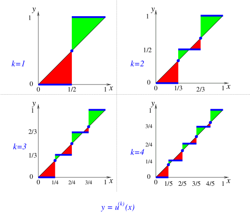
Figure 1: Win and loss zones for $u^{(k)}$

The following class of dual feasible functions is the implicit basis for the bin packing bound $L_{2}$ by Martello and Toth [17, 18]. This bound is obtained by neglecting all items smaller than a given value $\epsilon$. We account for these savings by increasing all items of size larger than $1-\epsilon$. Figure 2 shows the corresponding win and loss zones.

Proposition 4

Let $\epsilon\in[0,\frac{1}{2}]$. Then

$$U^{(\epsilon)}:[0,1] \rightarrow [0,1]$$

$$x \mapsto \left\{\begin{array}[]{ll}1,&\mbox{ for }x>1-\epsilon\\ x,&\mbox{ for }\epsilon\leq x\leq 1-\epsilon\\ 0,&\mbox{ for }x<\epsilon\end{array}\right.$$

is a dual feasible function. (See Figure 2.)

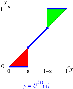
Figure 2: Win and loss zones for $U^{(\epsilon)}$

In our paper [6], we show how these two classes of dual feasible functions can be combined by virtue of Lemma 2 in order to get good bounds for the one-dimensional BPP. Our family of lower bounds can be computed in time $O(n)$ after sorting the items by size, and it dominates the class $L_{2}$ that was suggested by Martello an Toth [17, 18] as a generalization of the volume bound $L_{1}$. Our framework of dual feasible functions allows an easy generalization and proof of these bounds. In [6], we show that this generalized bound improves the asymptotic worst-case performance from $\frac{2}{3}$ to $\frac{3}{4}$, and provide empirical evidence that also the practical performance is improved significantly.

Our third class of dual feasible functions has some similarities to some bounds that were hand-tailored for the two-dimensional and three-dimensional BPP by Martello and Vigo [19], and Martello, Pisinger, and Vigo [16]. However, our bounds are simpler and dominate theirs. (We will discuss this in detail in Section 5.)

This third class also ignores items of size below a threshold value $\epsilon$. For the interval $(\epsilon,\frac{1}{2}]$, these functions are constant, on $(\frac{1}{2},1]$ they have the form of step functions. Figure 3 shows that for small values of $\epsilon$, the area of loss zones for $\phi^{(\epsilon)}$ exceeds the area of win zones by a clear margin. This contrasts to the behavior of the functions $u^{(k)}$ and $U^{(\epsilon)}$, where the win and loss areas have the same size.

Theorem 5

Let $\epsilon\in[0,\frac{1}{2})$. Then

$$\phi^{(\epsilon)}:[0,1] \rightarrow [0,1]$$

$$x \mapsto \left\{\begin{array}[]{ll}1-\frac{\lfloor(1-x)\epsilon^{-1}\rfloor}{\lfloor\epsilon^{-1}\rfloor},&\mbox{ for }x>\frac{1}{2}\\ \frac{1}{\lfloor\epsilon^{-1}\rfloor},&\mbox{ for }\epsilon\leq x\leq\frac{1}{2}\\ 0,&\mbox{ for }x<\epsilon\end{array}\right.$$

is a dual feasible function. (See Figure 3.)

Figure 3: Win and loss zones for $\phi^{(\epsilon)}$

Proof:   Let $S$ be a finite set of nonnegative real numbers, with $\sum\limits_{x\in S}x\leq 1$. Let $S^{\prime}:=\{x\in S\,|\,\epsilon\leq x\leq\frac{1}{2}\}.$ We distinguish two cases:

If all elements of $S$ have size at most $\frac{1}{2}$, then by definition of $S^{\prime}$,

$$1\geq\sum_{x\in S}x\geq\sum_{x\in S^{\prime}}x\geq|S^{\prime}|\epsilon$$ (5)

holds. Since $|S^{\prime}|$ is integral, it follows that $|S^{\prime}|\leq\lfloor\epsilon^{-1}\rfloor$, hence

$$\sum_{x\in S}\phi^{(\epsilon)}(x)=\sum_{x\in S^{\prime}}\phi^{(\epsilon)}(x)=|S^{\prime}|\frac{1}{\lfloor\epsilon^{-1}\rfloor}\leq 1.$$ (6)

Otherwise $S$ contains exactly one element $y>\frac{1}{2}$ and we have

$$1\geq\sum_{x\in S}x\geq y+\sum_{x\in S^{\prime}}x\geq y+|S^{\prime}|\epsilon.$$ (7)

Therefore $|S^{\prime}|\leq\lfloor(1-y)\epsilon^{-1}\rfloor$ and hence

$$\sum_{x\in S}\phi^{(\epsilon)}(x)=\phi^{(\epsilon)}(y)+\sum_{x\in S^{\prime}}\phi^{(\epsilon)}(x)=1-\frac{\lfloor(1-y)\epsilon^{-1}\rfloor}{\lfloor\epsilon^{-1}\rfloor}+|S^{\prime}|\frac{1}{\lfloor\epsilon^{-1}\rfloor}\leq 1.$$ (8)

 $\Box$

4 Conservative Scales

In this section we return to our original goal: deducing necessary conditions for feasible packings.

There can only be a packing if the total volume of the boxes does not exceed the volume of the container. This trivial necessary criterion is called the volume criterion. As we will see, it remains valid even if we apply appropriate transformations on the box sizes.

For any coordinate $i$, let

$${\cal F}(V,w_{i}):=\{S\subseteq V|w_{i}(S)\leq 1\},\,i\in\{1,\dots,d\}$$

be the family of $i$-feasible box sets, i.e., the subsets of boxes whose total $i$-width does not exceed the width of the container. If we replace $w$ by a size function $w^{\prime}$ without reducing these families, then all packing classes remain intact:

Theorem 6

Let $(V,w)$ and $(V,w^{\prime})$ be OPP instances. If for all $i\in\{1,\dots,d\}$ we have

$${\cal F}(V,w_{i})\subseteq{\cal F}(V,w^{\prime}_{i}),$$ (9)

then any packing class for $(V,w)$ is also a packing class for $(V,w^{\prime})$.

Proof:  As we showed in our paper [3], the existence of a packing is equivalent to the existence of a packing class, i.e., a set of $d$ graphs $G_{i}=(V,E_{i}),i=1,\ldots,d$ that have the following properties:

$$(P1): G_{i}:=(V,E_{i})$$ Each is an interval graph.

$$(P2): \mbox{Each stable set }S\mbox{ of }G_{i}\mbox{ is $x_{i}$--feasible}.$$

$$(P3): \bigcap_{i=1}^{d}E_{i}=\emptyset.$$

(Intuitively, these graphs describe the overlap of the $i$-projections of the boxes.)

This means we can focus on packing classes. The only condition on a packing class that involves the size of the objects deals with condition (P2): Any stable set of one of the component graphs $G_{i}$ should be $i$-feasible, i.e., the total sum of $i$-widths should not exceed the $i$-width of the container. This means that an OPP instance is characterized by the families of $i$-feasible box sets. By assumption, these are not changed when replacing $w$ by $w^{\prime}$.  $\Box$

Definition 7 (Conservative Scales)

A function $w^{\prime}$ satisfying the conditions of Theorem 6 is called a conservative scale for $(V,w)$.

The desired generalization of the volume criterion follows directly from Theorem 6:

Corollary 8

If $w^{\prime}$ s a conservative scale for the OPP-instance $(V,w)$, then

$$\sum_{b\in V}{\mbox{\it vol}}_{w^{\prime}}(b)\leq 1$$ (10)

is a necessary condition for the existence of a packing class for $(V,w)$.

In order to apply the new criterion, we need a method for constructing functions $w^{\prime}$. A particular way of getting conservative scales is given by the dual feasible functions described in the previous section.

Lemma 9

Let $(V,w)$ be an OPP instance and let $u_{1},\dots,u_{d}$ be dual feasible functions. Then $w^{\prime}:=(u_{1}(w_{1})$, $\dots$, $u_{d}(w_{d}))$ is a conservative scale for $(V,w)$.

Proof: For $i\in\{1,\dots,d\}$ the functions $u_{i}$ are dual feasible, hence

$$S\in{\cal F}(V,w_{i})\,\Leftrightarrow\,\sum_{b\in S}w_{i}(b)\leq 1\,\Rightarrow\,\sum_{b\in S}u_{i}(w_{i}(b))\leq 1\,\Leftrightarrow\,S\in{\cal F}(V,w^{\prime}_{i}).$$

 $\Box$

In the previous section, we described the dual feasible functions $u^{(k)},\,k\in{\rm I\kern-1.79993ptN},$ that can be computed in constant time for any item. They can be used to construct a conservative scale for an OPP instance in $d\cdot|V|$-linear time. By checking the volume criterion for a small set of conservative scales, we get a fast heuristic method for identifying OPP instances without a feasible packing.

Example 10

Consider the three-dimensional OPP

“Do nine cubes of size $\frac{2}{5}$ fit into a unit cube container?”.

The total volume is $9\times\frac{8}{125}=0.576\leq 1$, hence the volume criterion does not produce an answer. By applying the dual feasible function $u^{(2)}$ to all components, we get a conservative scale. The transformed boxes are cubes of size $\frac{1}{2}$. Now the total volume is $9\times\frac{1}{8}=1.125>1$, so with the help of Corollary 8, we get the answer “no” to the original question.

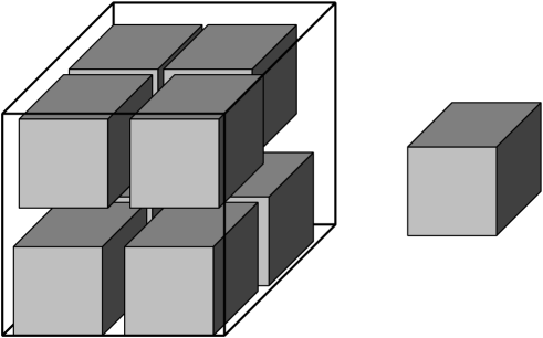
Figure 4: Trying to fit nine cubes of size $0.4$ into a unit container. (Example 10)

5 Bounds for Orthogonal Packing Problems

Corollary 8 yields a generic method for deriving linear relaxations of orthogonal packing problems: Let ${\cal W}$ be an arbitrary set of conservative scales for $(V,w)$. Then the difficult constraint

$$\mbox{``There is a packing class for }(S,w)\mbox{''}$$

can be replaced by the linear restriction

$$\forall w^{\prime}\in{\cal W}:\,{\mbox{\it vol}}_{w^{\prime}}(S)\leq 1.$$

The corollary implies that the latter is a relaxation. In the following we will use this method to obtain bounds for all orthogonal packing problems.

5.1 Strip Packing Problem

For the SPP-$d$, we get a lower bound:

Lemma 11

Let $V$ be a set of boxes, let $w$ be a size function on $V$, and let ${\cal W}$ be a finite set of conservative scales for $(V,w)$. Then the function $L_{SPP}(V,w)$, defined by

$$L_{SPP}(V,w):=\max_{w^{\prime}\in{\cal W}}{\mbox{\it vol}}_{w^{\prime}}(V),$$

is a lower bound for the SPP instance $(V,w)$.

The proof is immediate.

If a conservative scale $w^{\prime}$ is composed from dual feasible functions as described in Section 3, which can be evaluated in constant time for each box, then $L_{SPP}(V,w^{\prime})$ can be computed in time that is linear in $d\cdot|V|$.

5.2 Orthogonal Knapsack Problem

By using the above relaxation, the OKP turns into a higher-dimensional knapsack problem (MKP) (see [9]). While the OKP is strongly NP-hard, the MKP can be solved in pseudopolynomial time by using the dynamic program for the one-dimensional problem.

In case of ${\cal W}=\{w^{\prime}\}$ we get a one-dimensional knapsack problem as an OKP relaxation, with item weights given by box volumes with respect to the conservative scale $w^{\prime}$, and capacity given by the volume of the container. These bounds are used in the implementation of our OKP algorithm, which is described in detail in our paper [5]

5.3 Orthogonal Bin Packing Problem

The OBPP is relaxed to a Vector Packing Problem (see [10],[11]). This problem is still strongly NP-hard.

In order to derive a bound for the OBPP that is easier to compute, we consider the continuous lower bound $L_{0}$ for the one-dimensional BPP. For unit capacity, this bound arises as the sum of item sizes, rounded up to the next integer. $L_{0}$ yields a good approximation of the optimum, as long as there are sufficiently many “small” items (see [17, 18]).

For many instances, a majority of boxes has at least one dimension that is significantly smaller than the size of the container. This means that the box volume is significantly smaller than the volume of the container. In general, this is still true after a transformation by a conservative scale. This makes it plausible to use $L_{0}$ on transformed volumes. Summarizing:

Lemma 12

Let $V$ be a set of boxes, let $w$ be a size function on $V$, and let ${\cal W}$ be a finite set of conservative scales for $(V,w)$. Then the function $L_{OBPP}(V,w)$, defined by

$$L_{OBPP}(V,w):=\max_{w^{\prime}\in{\cal W}}\lceil{\mbox{\it vol}}_{w^{\prime}}(V)\rceil,$$

is a lower bound for the normalized OBPP instance $(V,w)$.

For conservative scales $w^{\prime}$ that are composed from dual feasible functions as described in Section 3, $L_{OBPP}(V,w^{\prime})$ can be computed in time linear in $d\cdot|V|$ — just like the bounds for strip packing from Lemma 11.

We demonstrate the advantages of our method by showing that generalizations of the lower bounds for the OBPP-$2$ and the OBPP-$3$ from the papers by Martello and Vigo [19] and Martello, Pisinger, and Vigo [16] fit into this framework. Those bounds are stated as maxima of several partial bounds that can all be stated as in Lemma 12. The necessary conservative scales can all be constructed from dual feasible functions $u^{(1)},U^{(\epsilon)}$ and $\phi^{(\epsilon)}$. In [19] and [16], these partial bounds are all derived by separate considerations, some of which are quite involved. We will discuss two of these cases to demonstrate how our framework leads to a better understanding of bounds and helps to find improvements. Particularly useful for this purpose is the decomposition of bounds into independent one-dimensional components, which was established in Lemma 9.

We state the original formulation of the most complicated partial bound in [19]. The only modification (apart from the naming of variables) arises from applying their bound to the normalized OBPP-$2$. (The integrality of input data that is required in [19] is of no consequence in this context.) For two parameters $p,q\in(0,\frac{1}{2}]$, Martello and Vigo set

$$I_{1}(p,q) := \left\{b\in V\quad|\quad w_{1}(b)>1-p\quad\wedge\quad w_{2}(b)>1-q\right\},$$

$$I_{2}(p,q) := \left\{b\in V\setminus I_{1}(p,q)\quad|\quad w_{1}(b)>\frac{1}{2}\quad\wedge\quad w_{2}(b)>\frac{1}{2}\right\},$$

$$I_{3}(p,q) := \left\{b\in V\quad|\quad\frac{1}{2}\geq w_{1}(b)\geq p\quad\wedge\quad\frac{1}{2}\geq w_{2}(b)\geq q\right\},$$

$$m(b,p,q):=\left\lfloor\frac{1}{p}\right\rfloor\left\lfloor\frac{1-w_{2}(b)}{q}\right\rfloor+\left\lfloor\frac{1}{q}\right\rfloor\left\lfloor\frac{1-w_{1}(b)}{p}\right\rfloor-\left\lfloor\frac{1-w_{1}(b)}{p}\right\rfloor\left\lfloor\frac{1-w_{2}(b)}{q}\right\rfloor,$$

$$L^{(p,q)}(V,w):=|I_{1}(p,q)\cup I_{2}(p,q)|+\left\lceil\frac{|I_{3}(p,q)|-\sum_{b\in I_{2}(p,q)}m(b,p,q)}{\lfloor p^{-1}\rfloor\lfloor q^{-1}\rfloor}\right\rceil.$$

Martello and Vigo derive the bound $L^{(p,q)}$ (which is denoted by $L_{3}(p,q)$ in [19]) by a geometric argument that uses a certain type of normal form of two-dimensional packings. This implies that only boxes from the sets $I_{1}(p,q)$, $I_{2}(p,q)$, $I_{3}(p,q)$ are taken into account.

We now give a formulation according to Lemma 12 that uses a conservative scale.

Theorem 13

Let $p,q\in(0,\frac{1}{2}]$. With

$$w^{\prime(p,q)}:=(\phi^{(p)}\circ w_{1},\phi^{(q)}\circ w_{2})$$

we have

$$L^{(p,q)}(V,w)=\lceil{\mbox{\it vol}}_{w^{\prime(p,q)}}(I_{1}(p,q)\cup I_{2}(p,q)\cup I_{3}(p,q))\rceil.$$

Proof.

In the following we only use elementary transformations and the definition of the dual feasible functions $\phi^{(\epsilon)}$ from Theorem 5.

By definition of $I_{1}(p,q)$ and $I_{3}(p,q)$ it follows immediately that

$$\forall b\in I_{1}(p,q):{\mbox{\it vol}}_{w^{\prime(p,q)}}(b)=1\cdot 1=1$$

and

$$\forall b\in I_{3}(p,q):{\mbox{\it vol}}_{w^{\prime(p,q)}}(b)=\frac{1}{\lfloor p^{-1}\rfloor}\frac{1}{\lfloor q^{-1}\rfloor}.$$

Furthermore, we get for $b\in I_{2}(p,q)$

$${\mbox{\it vol}}_{w^{\prime(p,q)}}(b)\quad=\quad\phi^{(p)}(w_{1}(b))\cdot\phi^{(q)}(w_{2}(b))$$

$$= \left(1-\frac{\lfloor(1-w_{1}(b))p^{-1}\rfloor}{\lfloor p^{-1}\rfloor}\right)\left(1-\frac{\lfloor(1-w_{2}(b))q^{-1}\rfloor}{\lfloor q^{-1}\rfloor}\right)$$

$$= 1-\frac{\lfloor(1-w_{1}(b))p^{-1}\rfloor}{\lfloor p^{-1}\rfloor}-\frac{\lfloor(1-w_{2}(b))q^{-1}\rfloor}{\lfloor q^{-1}\rfloor}+\frac{\lfloor(1-w_{1}(b))p^{-1}\rfloor\lfloor(1-w_{2}(b))q^{-1}\rfloor}{\lfloor p^{-1}\rfloor\lfloor q^{-1}\rfloor}$$

$$= 1-\frac{\left(\left\lfloor\frac{1}{q}\right\rfloor\left\lfloor\frac{(1-w_{1}(b))}{p}\right\rfloor+\left\lfloor\frac{1}{p}\right\rfloor\left\lfloor\frac{(1-w_{2}(b))}{q}\right\rfloor-\left\lfloor\frac{(1-w_{1}(b))}{p}\right\rfloor\left\lfloor\frac{(1-w_{2}(b))}{q}\right\rfloor\right)}{\lfloor p^{-1}\rfloor\lfloor q^{-1}\rfloor}$$

$$= 1-\frac{m(b,p,q)}{\lfloor p^{-1}\rfloor\lfloor q^{-1}\rfloor}.$$

All in all, this yields:

$$\lceil{\mbox{\it vol}}_{w^{\prime(p,q)}}(I_{1}(p,q)\cup I_{2}(p,q)\cup I_{3}(p,q))\rceil$$

$$= \left\lceil\sum_{b\in I_{1}(p,q)}{\mbox{\it vol}}_{w^{\prime(p,q)}}(b)+\sum_{b\in I_{2}(p,q)}{\mbox{\it vol}}_{w^{\prime(p,q)}}(b)+\sum_{b\in I_{3}(p,q)}{\mbox{\it vol}}_{w^{\prime(p,q)}}(b)\right\rceil$$

$$= \left\lceil\sum_{b\in I_{1}(p,q)}1+\sum_{b\in I_{2}(p,q)}\left(1-\frac{m(b,p,q)}{\lfloor p^{-1}\rfloor\lfloor q^{-1}\rfloor}\right)+\sum_{b\in I_{3}(p,q)}\frac{1}{\lfloor p^{-1}\rfloor\lfloor q^{-1}\rfloor}\right\rceil$$

$$= \left\lceil|I_{1}(p,q)|+|I_{2}(p,q)|-\sum_{b\in I_{2}(p,q)}\frac{m(b,p,q)}{\lfloor p^{-1}\rfloor\lfloor q^{-1}\rfloor}+\frac{I_{3}(p,q)}{\lfloor p^{-1}\rfloor\lfloor q^{-1}\rfloor}\right\rceil$$

$$= L^{(p,q)}(V,w).$$

 $\Box$

This alternative formulation of $L^{(p,q)}$ from Theorem 13 reveals a significant disadvantage of the bound: Boxes that are not contained in one of the sets $I_{1}(p,q),I_{2}(p,q),I_{3}(p,q)$ are disregarded for the balance, even if their volume is positive with respect to $w^{\prime(p,q)}$. In particular, boxes are disregarded that are narrow in one coordinate direction ($w_{i}(b)\leq\frac{1}{2}$) and wide in the other ($w_{i}(b)>\frac{1}{2}$). For example, the OBPP-$2$ instance with

$$V:=\{b_{1},b_{2},b_{3}\},\quad w(b_{1}):=\left(\frac{2}{3},\frac{1}{2}\right),\,w(b_{2})=w(b_{3}):=\left(\frac{1}{2},\frac{2}{3}\right)$$

yields $L^{(p,q)}(V,w)=0$ for all $p,q\in(0,\frac{1}{2}]$. None of the other partial bounds from [19] exceed the value of $1$. However, the above discussion yields the following improvement of $L^{(p,q)}$:

$$L^{\prime(p,q)}(V,w)=\lceil{\mbox{\it vol}}_{w^{\prime(p,q)}}(V)\rceil$$

This yields $L^{\prime(\frac{1}{2},\frac{1}{2})}(V,w)=2$, which is the optimal value.

We now give a description of the OBPP bound from [19] with the above improvement in the framework of conservative scales. Like the proof of Theorem 13, it can be derived by using only the definition of conservative scales and elementary transformations.

Theorem 14

For $p,q\in(0,\frac{1}{2}]$ let

$$\begin{array}[]{lccrrc}w^{(1)(p)}&:=&(&u^{(1)}\circ w_{1},&U^{(p)}\circ w_{2}&),\\ w^{(2)(p)}&:=&(&U^{(p)}\circ w_{1},&u^{(1)}\circ w_{2}&),\\[4.30554pt] w^{(3)(p)}&:=&(&u^{(1)}\circ w_{1},&\phi^{(p)}\circ w_{2}&),\\ w^{(4)(p)}&:=&(&\phi^{(p)}\circ w_{1},&u^{(1)}\circ w_{2}&),\\[4.30554pt] w^{(5)(p)}&:=&(&w_{1},&U^{(p)}\circ w_{2}&),\\ w^{(6)(p)}&:=&(&U^{(p)}\circ w_{1},&w_{2}&),\\[4.30554pt] w^{(7)(p,q)}&:=&(&\phi^{(p)}\circ w_{1},&\phi^{(q)}\circ w_{2}&).\end{array}$$

By Lemma 12, the maximum over the partial bounds is

$$L_{2d}:=\max\left\{\max_{k\in\{1,\dots,6\}}\max_{0<p\leq\frac{1}{2}}\{\lceil{\mbox{\it vol}}_{w^{(k)(p)}}(V)\rceil\},\max_{0<p\leq\frac{1}{2},\,0<q\leq\frac{1}{2}}\{\lceil{\mbox{\it vol}}_{w^{(7)(p,q)}}(V)\rceil\}\right\}.$$

$L_{2d}$ dominates the bound $L_{4}$ from [19].

Like for the bound $L_{2}$ (see Martello and Toth [17]), finding the maxima over the parameters $p,q$ can be reduced to considering finitely many values. This makes it possible to compute the one-parametric bounds in time $O(|V|)$, and the two-parametric bound in time $O(|V|^{2})$, provided that the boxes are sorted by size for each coordinate direction.

Most partial bounds for the OKP-$3$ that are given in [16] disregard boxes that do not span at least half the container volume in two coordinate directions. Since these boxes have to be stacked in the third direction, it is possible to use the corresponding bounds for the one-dimensional BPP.

Not counting symmetry, there is only one partial bound in [16] that is really based on higher-dimensional properties. For this bound, we derive a dominating new bound in terms of conservative scales.

For this purpose, let $p,q\in(0,\frac{1}{2}]$ and consider the sets

$$J_{1}(p,q) := \left\{b\in V\quad|\quad w_{1}(b)>1-p\quad\wedge\quad w_{2}(b)>1-q\right\},$$

$$J_{2}(p,q) := \left\{b\in V\setminus J_{1}(p,q)\quad|\quad w_{1}(b)>p\quad\wedge\quad w_{2}(b)>q\right\}.$$

A simplified formulation of the lower bound for the normalized OBPP-$3$ is

$$L^{(p,q)}(V,w):=\left\lceil\sum_{b\in J_{1}(p,q)}w_{3}(b)+\sum_{b\in J_{2}(p,q)}{\mbox{\it vol}}_{w}(b)\right\rceil.$$

In the first two coordinate directions, the size of the box is rounded to the full size of the container, if and only if both sizes exceed their respective threshold values $(1-p)$ and $(1-q)$. Noting that the same effect can be reached in each dimension by using the dual feasible function $U^{(\epsilon)}$, we see that the interconnection between both directions is unnecessary. Using the conservative scale

$$w^{\prime(p,q)}:=(U^{(p)}\circ w_{1},U^{(q)}\circ w_{2},w_{3}),$$

we can round up both sizes in the same way, but independent from each other. This yields the following bound that dominates $L^{(p,q)}$:

$$L^{\prime(p,q)}(V,w):=\left\lceil w^{\prime(p,q)}(V)\right\rceil.$$

For an example that there is some improvement, consider the OBPP-$3$ instance $(V,w)$ with five boxes of sizes $\left(\frac{2}{3},\frac{1}{2},\frac{1}{2}\right)$. For all $p,q\in(0,\frac{1}{2}]$ the set $J_{1}(p,q)$ is empty, so that $L^{(p,q)}(V,w)\leq\lceil{\mbox{\it vol}}_{w}(V)\rceil=\left\lceil\frac{5}{6}\right\rceil=1$ holds. On the other hand, $L^{\prime(p,q)}(V,w)=\lceil\frac{5}{4}\rceil=2$ yields the optimal value.

All other partial bounds from [16] can be formulated as in Lemma 12. The proof is left to the reader.

Theorem 15

Using the following conservative scales, we get a description of the bound from [16], including the improvement mentioned above.

$$\begin{array}[]{lccrrrc}w^{(1)(p)}&:=&(&u^{(1)}\circ w_{1},&u^{(1)}\circ w_{2},&U^{(p)}\circ w_{3}&),\\ w^{(2)(p)}&:=&(&u^{(1)}\circ w_{1},&U^{(p)}\circ w_{2},&u^{(1)}\circ w_{3}&),\\ w^{(3)(p)}&:=&(&U^{(p)}\circ w_{1},&u^{(1)}\circ w_{2},&u^{(1)}\circ w_{3}&),\\[4.30554pt] w^{(4)(p)}&:=&(&u^{(1)}\circ w_{1},&u^{(1)}\circ w_{2},&\phi^{(p)}\circ w_{3}&),\\ w^{(5)(p)}&:=&(&u^{(1)}\circ w_{1},&\phi^{(p)}\circ w_{2},&u^{(1)}\circ w_{3}&),\\ w^{(6)(p)}&:=&(&\phi^{(p)}\circ w_{1},&u^{(1)}\circ w_{2},&u^{(1)}\circ w_{3}&),\\[4.30554pt] w^{(7)(p,q)}&:=&(&U^{(p)}\circ w_{1},&U^{(q)}\circ w_{2},&w_{3}&),\\ w^{(8)(p,q)}&:=&(&U^{(p)}\circ w_{1},&w_{2},&U^{(q)}\circ w_{3}&),\\ w^{(9)(p,q)}&:=&(&w_{1},&U^{(p)}\circ w_{2},&U^{(q)}\circ w_{3}&).\end{array}$$

Then the maximum of the corresponding partial bounds according to Lemma 12 is

$$L_{3d}(V,w):=\max\left\{\max_{k\in\{1,\dots,6\}}\max_{0<p\leq\frac{1}{2}}\{\lceil{\mbox{\it vol}}_{w^{(k)(p)}}(V)\rceil\},\max_{k\in\{7,\dots,9\}}\max_{0<p\leq\frac{1}{2},\,0<q\leq\frac{1}{2}}\{\lceil{\mbox{\it vol}}_{w^{(k)(p,q)}}(V)\rceil\}.\right\}$$

This dominates the bound $L_{2}$ from [16].

Like $L_{2d}$, $L_{3d}$ can be computed in quadratic time.

From the new formulation of $L_{2d}$ and $L_{3d}$ it is immediate how the bounds can be improved by applying further dual feasible functions, without changing the complexity. $u^{(1)},U^{(\epsilon)}$, and $\phi^{(\epsilon)}$ are all dual feasible functions with win zones in the interval $(\frac{1}{2},1]$. (See Figures 1, 2, 3). This suggests it may be a good idea to use $u^{(k)},k\geq 2$ as well, where sizes $\leq\frac{1}{2}$ may be rounded up.

6 Bounds for Packing Classes

As mentioned in the proof of Theorem 6, and described in detail in our paper [3], it suffices to construct packing classes instead of explicit feasible geometric arrangements of boxes. This allows us to enumerate over feasible packings by performing a branch-and-bound scheme over the edge sets of the component graphs $G_{i}=(V,E_{i})$. At each stage of this scheme, we have fixed a subset of edges ${\cal E}_{+,i}\subseteq E_{i},\,i=1,\dots,d$ to be in the $i$th component graph $G_{i}$.

In the following, we describe how conservative scales can be used for constructing bounds on partial edge sets. In our exact algorithm that is described in [5], they help to limit the growth of the search tree.

First of all, conservative scales can be used to weaken the assumptions of Theorem 9 from our paper [3]:

Theorem 16

Let $E$ be a packing class for $(V,w)$, $w^{\prime}$ be a conservative scale for $(V,w)$, $i\in\{1,\dots,d\}$ and $S\subseteq V$. Let $G_{i}$ be the $i$th component graph of $E$. Then $G_{i}[S]$ contains a clique of cardinality $\lceil w^{\prime}_{i}(S)\rceil$.

Proof: By Theorem 6, any packing class $E$ for $(V,w)$ is also a packing class for $(V,w^{\prime})$. Then the claim follows from Theorem 9 in [3].  $\Box$

Now we generalize conservative scales. We assume that only packing classes $E$ are relevant that satisfy the condition

$${\cal E}_{+,i}\subseteq E_{i},\,i=1,\dots,d,$$ (11)

where ${\cal E}_{+,1}\dots,{\cal E}_{+,d}$ are given edge sets on $V$.

Consider a set of boxes $S\subseteq V$ that contains two boxes $b,c$, such that $e=bc\in{\cal E}_{+,i}$. With $e$, at least one of the edges of the clique $E_{S}$ must be contained in the $i$th component graph of any relevant packing class. This implies that $S$ can never occur as an independent set of the $i$th component graph in condition (P2). Therefore, $i$-feasibility of $S$ is not an issue, so removal of $S$ from ${\cal F}(V,w_{i})$ cannot delete any relevant packing classes. This means that for the purpose of size modification, we only have to consider sets of boxes $S$ with cliques $E_{S}$ that are disjoint from ${\cal E}_{+,i}$. The family of these sets is denoted by

$${\cal F}(V,w_{i},{\cal E}_{+,i}):=\left\{S\in{\cal F}(V,w_{i})|\mbox{$E_{S}$}\cap{\cal E}_{+,i}=\emptyset\right\}.$$

Therefore, the assumptions of Theorem 6 can be weakened:

Theorem 17

Let $(V,w)$ and $(V,w^{\prime})$ be OPP-$d$ instances, let ${\cal E}_{+}=({\cal E}_{+,1}\dots,{\cal E}_{+,d})$ be $d$-tuples of edge sets on $V$, and let $E$ be a packing class of $(V,w)$ that satisfies (11). Suppose that for all $i\in\{1,\dots,d\}$ the following holds:

$${\cal F}(V,w_{i},{\cal E}_{+,i})\subseteq{\cal F}(V,w^{\prime}_{i}).$$ (12)

Then $E$ is a packing class for $(V,w^{\prime})$.

Proof. Like in the proof for Theorem 6 we only have to check condition (P2). By (11) any independent set $S$ of the $i^{th}$ component graph satisfies $\mbox{$E_{S}$}\cap{\cal E}_{i}=\emptyset$. Then the assumption (12) guarantees that (P2) remains valid when changing $w$ to $w^{\prime}$.  $\Box$

Definition 18 (Generalization of Definition 7)

Given the assumptions of Theorem 17. Then we say that $w^{\prime}$ is a conservative scale for $(V,w,{\cal E}_{+})$.

Definitions 7 and 18 are compatible. A conservative scale for $(V,w,(\emptyset,\dots,\emptyset))$ is a conservative scale for $(V,w)$. Conversely, a conservative scale for $(V,w)$ is a a conservative scale for $(V,w,{\cal E}_{+})$ for any $d$-tuple of edge sets ${\cal E}_{+}$ of $V$.

Corollary 8 can now be generalized:

Corollary 19

Let $w^{\prime}$ be a conservative scale for $(V,w,{\cal E}_{+})$. Then condition (10) from Corollary 8 is a sufficient condition for the existence of a packing class for $(V,w)$ that satisfies condition (11).

So far we have used a selection of easily constructible conservative scales in order to apply the volume criterion. Now we describe a method for improving conservative scales by increasing the total box volume. Our approach uses the information provided by (11). The idea is to stretch an individual box along a given coordinate as much as possible while preserving a conservative scale.

Lemma 20

Let $(V,w)$ be an OPP-$d$ instance and let ${\cal E}_{+}$ be a $d$-tuple of edge sets on $V$. Let $b\in V$ be a box and let $i\in\{1,\dots,d\}$ be a coordinate direction. Choose

$$\lambda\geq\max\left\{w_{i}(S)\,|\,S\in{\cal F}(V,w_{i},{\cal E}_{+,i})\,\mbox{ and }\,b\in S\right\}.$$ (13)

Then the size function $w^{\prime}$ given by

$$w^{\prime}_{j}(c):=\left\{\begin{array}[]{ll}w_{j}(c)+(1-\lambda)&\mbox{ for }(j,c)=(i,b)\\ w_{j}(c)&\mbox{ else }\end{array}\right.$$ (14)

is a conservative scale for $(V,w,{\cal E}_{+})$.

Proof. Condition (12) needs to be checked only for coordinate $i$ and for sets containing $b$. Therefore consider a set $S\in{\cal F}(V,w_{i},{\cal E}_{+,i})$ with $b\in S$. Then the choice of $\lambda$ assures that

$$w^{\prime}_{i}(S)=w_{i}(S)+(1-\lambda)\leq w_{i}(S)+(1-w_{i}(S))=1.\hfill\hbox{\quad$\Box$ \vspace{1ex}}$$

It suffices to consider an upper bound for the maximum in (13) for these computations. For example, the family ${\cal F}(V,w_{i},{\cal E}_{+,i})$ is contained in the the power set of $\{b\}\cup\{c\in V\,|\,bc\in{\cal E}_{+,i}\}$. Replacing the family by the power set yields an upper bound that can be computed as the solution of a one-dimensional knapsack problem.

The following example illustrates the technical lemma and the underlying terms.

Example 21

Consider the OPP-$2$ instance $(V,w,W)$ with

$$V:=\left\{1^{\prime},\dots,6^{\prime}\right\},\quad W:=(20,13),$$

$$\begin{array}[]{rclrcl}w(1^{\prime})=w(2^{\prime})&:=&(8,7),&w(3^{\prime})&:=&(12,4),\\ w(4^{\prime})=w(5^{\prime})&:=&(6,6),&w(6^{\prime})&:=&(8,3).\\ \end{array}$$

Using Theorem 20, we construct a conservative scale that disproves the existence of a packing class with the side constraints

$$E_{1}\supseteq{\cal E}_{+,1}:=\{1^{\prime}3^{\prime},4^{\prime}5^{\prime}\}$$

.

We start by giving an intuitive idea of the situation. Let direction $1$ be “horizontal” and let direction $2$ be “vertical”. For a packing class, consider the space right and left of box $1^{\prime}$:

• Box $3^{\prime}$ must be outside of this space, as it is adjacent to $1^{\prime}$ in in ${\cal E}_{+,1}$; this implies a horizontal overlap with $1^{\prime}$.

• If $2^{\prime}$ or $6^{\prime}$ are packed alongside $1^{\prime}$, horizontal free space of size $W_{1}-w_{1}(1^{\prime})-w_{1}(2^{\prime})=W_{1}-w_{1}(1^{\prime})-w_{1}(6^{\prime})=20-8-8=4$ is left at the respective level, which does not fit any further boxes.

• $4^{\prime}$ and $5^{\prime}$ would both fit next to $1^{\prime}$. Because of $4^{\prime}5^{\prime}\in{\cal E}_{+,1}$, one of these boxes must lie above the other. This means that at most one of the boxes $4^{\prime}$ and $5^{\prime}$ is packed alongside $1^{\prime}$, leaving horizontal free space of size $W_{1}-w_{1}(1^{\prime})-w_{1}(4^{\prime})=W_{1}-w_{1}(1^{\prime})-w_{1}(5^{\prime})=20-8-6=6$.

At any level right and left of box $1^{\prime}$, at least a total of $4$ units must remain free. This implies an unpacked space of size at least $4\cdot 7$.

These facts can be covered by the terminology of conservative scales:

The maximal sets from ${\cal F}(V,w_{1},{\cal E}_{+,1})$ that contain $1^{\prime}$ are

$$\{1^{\prime},2^{\prime}\},\{1^{\prime},4^{\prime}\},\{1^{\prime},5^{\prime}\},\{1^{\prime},6^{\prime}\}.$$

This implies

$$\max\{w_{1}(S)|S\in{\cal F}(V,w_{1},{\cal E}_{+,i}),\,1^{\prime}\in S\}\,=\,\max\{8+8,\,8+8,\,8+6,\,8+6\}\,=\,16.$$

By Theorem 20 we get from $w$ a conservative scale for $(V,w,{\cal E}_{+})$by replacing $w_{1}(1^{\prime})=8$ by $8+(20-16)=12$. With respect to this conservative scale, the total box volume is

$$12\cdot 7+8\cdot 7+12\cdot 4+6\cdot 6+6\cdot 6+8\cdot 3=284>20\cdot 13=W_{1}\cdot W_{2}.$$

By Theorem 19, no packing class with $E_{1}\supseteq{\cal E}_{+,1}$ can exist.  $\Box$

7 Conclusions

We have described a new framework for obtaining lower bounds for higher-dimensional packing problems. We have shown that all known classes of lower bounds for these problems can easily be formulated in and improved by this framework. In this paper we have given three particular classes of dual feasible functions. Furthermore, any additional set of dual feasible functions for one-dimensional packing (described in detail in our paper [6]) can be used immediately for constructing new lower bounds for higher-dimensional packing problems, by using convex combinations and compositions.

When considering the performance of bounds resulting from dual feasible functions, one should also realize the limitations: As any such bound considers only one item at a time (which is why the bounds have linear complexity after sorting), complications resulting from the more involved combination of items cannot explicitly be recognized. Again, see [6] for a discussion in the context of one-dimensional bin packing. Thus, a possible way to stronger bounds may be to consider logical implications of several packed items at a time.

We omit a separate computational study on the performance of our new bounds. Instead, we demonstrate their usefulness by applying them to actually solve higher-dimensional packing problems to optimality. Combining our new classes of bounds with our characterization of feasible packings (described in [3, 7]), we get a powerful method that can solve instances of previously unmanageable size. All technical details are described in our paper [5].

References

- [1] S. P. Fekete, E. Köhler, and J. Teich. Higher-dimensional packing with order constraints. In Algorithms and Data Structures (WADS 2001), volume 2125 of Lecture Notes in Computer Science, pages 192–204. Springer-Verlag, 2001.
- [2] S. P. Fekete and J. Schepers. A new exact algorithm for general orthogonal d-dimensional knapsack problems. In Algorithms – ESA ’97, volume 1284 of Lecture Notes in Computer Science, pages 144–156. Springer-Verlag, 1997.
- [3] S. P. Fekete and J. Schepers. On higher-dimensional packing I: Modeling. Technical report, Univ. of Cologne, Center for Parallel Computing, Available at http://www.math.tu-bs.de/~fekete/ publications.html, 1997.
- [4] S. P. Fekete and J. Schepers. On higher-dimensional packing II: Bounds. Technical report, Univ. of Cologne, Center for Parallel Computing, Available at http://www.math.tu-bs.de/~fekete/ publications.html, 1997.
- [5] S. P. Fekete and J. Schepers. On higher-dimensional packing III: Exact algorithms. Technical report, Univ. of Cologne, Center for Parallel Computing, Available at http://www.math.tu-bs.de/ ~fekete/publications.html, 1997.
- [6] S. P. Fekete and J. Schepers. New classes of lower bounds for bin packing problems. Math. Programming, 91:11–32, 2001.
- [7] S. P. Fekete and J. Schepers. A combinatorial characterization of higher-dimensional orthogonal packing. Mathematics of Operations Research, 2004. to appear.
- [8] S. P. Fekete and J. Schepers. An exact algorithm for higher-dimensional orthogonal packing. Operations Research, 2004. to appear.
- [9] A. Freville and G. Plateau. An efficient preprocessing procedure for the multidimensional 0-1 knapsack problem. Discr. Appl. Math., 49:189–212, 1994.
- [10] G. Galambos, H. Kellerer, and G. J. Woeginger. A lower bound for on-line vector packing algorithms. Acta Cybern., 11:23–34, 1993.
- [11] M. R. Garey, R. L. Graham, D. S. Johnson, and A. C. Yao. Resource constrained scheduling as generalized bin packing. J. Combinatorial Theory Ser. A, 21:257–298, 1976.
- [12] D. S. Johnson. Near-optimal bin packing algorithms. PhD thesis, Massachusetts Institute of Technology, 1973.
- [13] E. G. Coffman jr. and G. S. Lueker. Probalistic Analysis of Packing and Partitioning Algorithms. Wiley, New York, 1991.
- [14] N. Kamarkar and R. M. Karp. An efficient approximation scheme for the one-dimensional bin-packing problem. In Proc. 23th IEEE Annu. Found. Comp. Sci. (FOCS 82), pages 312–320, 1982.
- [15] G. S. Lueker. Bin packing with items uniformly distributed over intervals . In Proc. 24th IEEE Annu. Found. Comp. Sci. (FOCS 83), pages 289–297, 1983.
- [16] S. Martello, D. Pisinger, and D. Vigo. The three-dimensional bin packing problem. Oper. Res., 48:256–267, 2000.
- [17] S. Martello and P. Toth. Knapsack Problems – Algorithms and Computer Implementations. Wiley, Chichester, 1990.
- [18] S. Martello and P. Toth. Lower bounds and reduction procedures for the bin packing problem. Discr. Appl. Math., 26:59–70, 1990.
- [19] S. Martello and D. Vigo. Exact solution of the two-dimensional finite bin packing problem. Managem. Sci., 44:388–399, 1998.