Heuristic average-case analysis of the backtrack resolution of random 3-Satisfiability instances.

Abstract

An analysis of the average-case complexity of solving random 3-Satisfiability (SAT) instances with backtrack algorithms is presented. We first interpret previous rigorous works in a unifying framework based on the statistical physics notions of dynamical trajectories, phase diagram and growth process. It is argued that, under the action of the Davis–Putnam–Loveland–Logemann (DPLL) algorithm, 3-SAT instances are turned into $2+p$-SAT instances whose characteristic parameters (ratio $\alpha$ of clauses per variable, fraction $p$ of 3-clauses) can be followed during the operation, and define resolution trajectories. Depending on the location of trajectories in the phase diagram of the 2+p-SAT model, easy (polynomial) or hard (exponential) resolutions are generated. Three regimes are identified, depending on the ratio $\alpha$ of the 3-SAT instance to be solved. Lower sat phase: for small ratios, DPLL almost surely finds a solution in a time growing linearly with the number $N$ of variables. Upper sat phase: for intermediate ratios, instances are almost surely satisfiable but finding a solution requires exponential time ($\sim 2^{N\,\omega}$ with $\omega>0$) with high probability. Unsat phase: for large ratios, there is almost always no solution and proofs of refutation are exponential. An analysis of the growth of the search tree in both upper sat and unsat regimes is presented, and allows us to estimate $\omega$ as a function of $\alpha$. This analysis is based on an exact relationship between the average size of the search tree and the powers of the evolution operator encoding the elementary steps of the search heuristic.

url]http://ludfc39.u-strasbg.fr/cocco/index.html

url]http://www.lptens.fr/$\sim$monasson

1 Introduction.

This paper focuses on the average complexity of solving random 3-SAT instances using backtrack algorithms. Being an NP-complete problem, 3-SAT is not thought to be solvable in an efficient way, i.e. in time growing at most polynomially with $N$. In practice, one therefore resorts to methods that need, a priori, exponentially large computational resources. One of these algorithms is the ubiquitous Davis–Putnam–Loveland–Logemann (DPLL) solving procedure(Davis, Logemann and Loveland, 1962; Gu, Purdom, Franco and Wah, 1997). DPLL is a complete search algorithm based on backtracking; its operation is briefly recalled in Figure 1. The sequence of assignments of variables made by DPLL in the course of instance solving can be represented as a search tree, whose size $Q$ (number of nodes) is a convenient measure of the hardness of resolution. Some examples of search trees are presented in Figure 2.

In the past few years, much experimental and theoretical progress has been made on the probabilistic analysis of 3-SAT (Hogg, Huberman and Williams, 1996; Gent, van Maaren and Walsh, 2000). Distributions of random instances controlled by few parameters are particularly useful in shedding light on the onset of complexity. An example that has attracted a lot of attention over the past years is random 3-SAT: all clauses are drawn randomly and each variable negated or left unchanged with equal probabilities. Experiments (Hogg, Huberman and Williams, 1996; Crawford and Auton, 1996; Mitchell, Selman and Levesque, 1992; Selman and Kirkpatrick, 1994) and theory (Friedgut, 1999; Dubois, Boufkhad and Mandler, 2000; Dubois et al., 2001) indicate that clauses can almost surely always (respectively never) be simultaneously satisfied if $\alpha$ is smaller (resp. larger) than a critical threshold $\alpha_{C}\simeq 4.3$ as soon as the numbers $M$ of clauses and $N$ of variables go to infinity at a fixed ratio $\alpha$. This phase transition (Monasson et al., 1999) is accompanied by a drastic peak in hardness at threshold (Hogg, Huberman and Williams, 1996; Mitchell, Selman and Levesque, 1992; Crawford and Auton, 1996). The emerging pattern of complexity is as follows. At small ratios $\alpha<\alpha_{L}$, where $\alpha_{L}$ depends on the heuristic used by DPLL, instances are almost surely satisfiable (sat), see Franco (2001) and Achlioptas (2001b) for recent reviews. The size $Q$ of the associated search tree scales, with high probability, linearly with the number $N$ of variables, and almost no backtracking is present (Frieze and Suen, 1996) (Figure 2A). Above the critical ratio, that is when $\alpha>\alpha_{C}$, instances are a.s. unsatisfiable (unsat) and proofs of refutation are obtained through massive backtracking (Figure 2B), leading to an exponential hardness: $Q=2^{N\omega}$ with $\omega>0$ (Chvàtal and Szmeredi, 1988). In the intermediate range, $\alpha_{L}<\alpha<\alpha_{C}$, finding a solution a.s. requires exponential effort ($\omega>0$) (Coarfa et al., 2000; Achlioptas, Beame and Molloy, 2001c; Cocco and Monasson, 2001).

The aim of this article is two-fold. First, we propose a simple and intuitive framework to unify the above findings. This framework is presented in Section 2. It is based on the statistical physics notions of dynamical trajectories and phase diagram, and was, to some extent, implicitly contained in the pioneering analysis of search heuristics by Chao and Franco (1986, 1990). Secondly, we present in Section 3 a quantitative study of the growth of the search tree in the unsat regime. Such a study has been lacking so far due to the formidable difficulty in taking into account the effect of massive backtracking on the operation of DPLL. We first establish an exact relationship between the average size of the search tree and the powers of the evolution operator encoding the elementary steps of the search heuristic. This equivalence is then used (in a non rigorous way) to accurately estimate the logarithm $\omega$ of the average complexity $Q$ as a function of $\alpha$,

$$\omega(\alpha)=\lim_{N\to\infty}\;\frac{1}{N}\;\log_{2}\;E_{(\alpha,N)}[Q]\quad,$$ (1)

where $E_{(N,\alpha)}$ denotes the expectation value for given $N$ and $\alpha$. The approach emphasizes the relevance of partial differential equations to analyse algorithms in presence of massive backtracking, as opposed to ordinary differential equations in the absence of the latter (Wormald, 1995; Achlioptas, 2001b). In Section 4, we focus upon the upper sat regime i.e. upon ratios $\alpha_{L}<\alpha<\alpha_{C}$. Combining the framework of Section 2 and the analysis of Section 3 we unveil the structure of the search tree (Figure 2C) and calculate $\omega$ as a function of the ratio $\alpha$ of the 3-SAT instance to be solved.

For the sake of clarity and since the style of our approach may look unusual to the computer scientist reader, the status of the different calculations and results (experimental, exact, conjectured, approximate, …) are made explicit throughout the article.

Figure 1: DPLL algorithm. When a variable has been chosen at step (1) e.g. $x=T$, at step (2) some clauses are satisfied e.g. $C=(x\;\hbox{\rm OR}\;{y}\;\hbox{\rm OR}\;z)$ and eliminated, other are reduced e.g. $C=(\hbox{\rm not}\,x\;\hbox{\rm OR}\;{y}\;\hbox{\rm OR}\;{z})\to C=({y}\;\hbox{\rm OR}\;{z})$. If some clauses include one variable only e.g. $C=y$, the corresponding variable is automatically fixed to satisfy the clause ($y=T$). This propagation (2c) is repeated up to the exhaustion of all unit clauses. Contradictions result from the presence of two opposite unit clauses e.g. $C=(y),C^{\prime}=(\hbox{\rm not}\,y)$. A solution is found when no clauses are left. The search process of DPLL is represented by a tree (Figure 2) whose nodes correspond to (1), and edges to (2). Branch extremities are marked with contradictions C (2B,2C), or by a solution S (2A,2C).

Figure 2: Types of search trees generated by the DPLL solving procedure on random 3-SAT. A. simple branch: the algorithm finds easily a solution without ever backtracking. B. dense tree: in the absence of solution, DPLL builds a tree, including many branches ending with contradictory leaves, before stopping. C. mixed case, branch + tree: if many contradictions arise before reaching a solution, the resulting search tree can be decomposed into a single branch followed by a dense tree. G is the highest node in the tree reached by DPLL through backtracking.

2 Phase diagram and trajectories.

2.1 The 2+p-SAT distribution and split heuristics

The action of DPLL on an instance of 3-SAT causes changes to the overall numbers of variables and clauses, and thus of the ratio $\alpha$. Furthermore, DPLL reduces some 3-clauses to 2-clauses. A mixed 2+p-SAT distribution, where $p$ is the fraction of 3-clauses, can be used to model what remains of the input instance at a node of the search tree. Using experiments and methods from statistical mechanics (Monasson et al., 1999), the threshold line $\alpha_{C}(p)$, separating sat from unsat phases, may be estimated with the results shown in Figure 3. For $p\leq p_{0}=2/5$, i.e. to the left of point T, the threshold line is given by $\alpha_{C}(p)=1/(1-p)$, as rigorously confirmed by Achlioptas et al. (2001a), and saturates the upper bound for the satisfaction of 2-clauses. Above $p_{0}$, no exact value for $\alpha_{C}(p)$ is known. Note that $\alpha_{C}\simeq 4.3$ corresponds to $p=1$.

The phase diagram of 2+p-SAT is the natural space in which DPLL dynamic takes place. An input 3-SAT instance with ratio $\alpha$ shows up on the right vertical boundary of Figure 3 as a point of coordinates $(p=1,\alpha)$. Under the action of DPLL, the representative point moves aside from the 3-SAT axis and follows a trajectory. This trajectory obviously depends on the heuristic of split followed by DPLL (Figure 1). Possible simple heuristics are (Chao and Franco, 1986, 1990),

• Unit-Clause (UC): randomly pick up a literal among a unit clause if any, or any unset variable otherwise.

• Generalized Unit-Clause (GUC): randomly pick up a literal among the shortest avalaible clauses.

• Short Clause With Majority (SC₁): randomly pick up a literal among unit clauses if any; otherwise randomly pick up an unset variable $v$, count the numbers of occurences $\ell,\bar{\ell}$ of $v$, $\bar{v}$ in 3-clauses, and choose $v$ (respectively $\bar{v}$) if $\ell>\bar{\ell}$ (resp. $\ell<\bar{\ell}$). When $\ell=\bar{\ell}$, $v$ and $\bar{v}$ are equally likely to be chosen.

Rigorous mathematical analysis, undertaken to provide rigorous bounds to the critical threshold $\alpha_{C}$, have so far been restricted to the action of DPLL prior to any backtracking, that is, to the first descent of the algorithm in the search tree. The corresponding search branch is drawn on Figure 2A. These studies rely on the two following facts:

First, the representative point of the instance treated by DPLL does not “leave” the 2+p-SAT phase diagram. In other words, the instance is, at any stage of the search process, uniformly distributed from the 2+p-SAT distribution conditioned to its clause–per–variable ratio $\alpha$ and fraction of 3-clauses $p$. This assumption is not true for all heuristics of split, but holds for the above examples ($UC$, $GUC$, $SC_{1}$) (Chao and Franco, 1986). Analysis of more sophisticated heuristics require to handle more complex instance distributions (Kaporis, Kirousis and Lalas, 2002).

Secondly, the trajectory followed by an instance in the course of resolution is a stochastic object, due to the randomness of the instance and of the assignments done by DPLL. In the large size limit ($N\to\infty$), this trajectory gets concentrated around its average locus in the 2+p-SAT phase diagram. This concentration phenomenon results from general properties of Markov chains (Wormald, 1995; Achlioptas, 2001b).

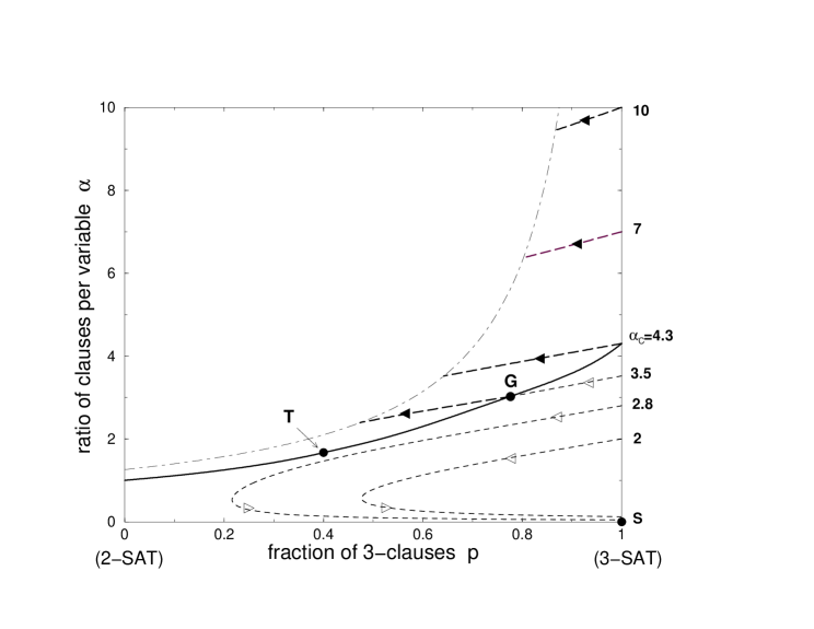
Figure 3: Phase diagram of 2+p-SAT and dynamical trajectories of DPLL. The threshold line $\alpha_{C}(p)$ (bold full line) separates sat (lower part of the plane) from unsat (upper part) phases. Extremities lie on the vertical 2-SAT (left) and 3-SAT (right) axis at coordinates ($p=0,\alpha_{C}=1$) and ($p=1,\alpha_{C}\simeq 4.3$) respectively. Departure points for DPLL trajectories are located on the 3-SAT vertical axis and the corresponding values of $\alpha$ are explicitely given. Dashed curves represent tree trajectories in the unsat region (thick lines, black arrows) and branch trajectories in the sat phase (thin lines, empty arrows). Arrows indicate the direction of ”motion” along trajectories parametrized by the fraction $t$ of variables set by DPLL. For small ratios $\alpha<\alpha_{L}$, branch trajectories remain confined in the sat phase, end in S of coordinates $(1,0)$, where a solution is found. At $\alpha_{L}$ ($\simeq 3.003$ for the GUC heuristic), the single branch trajectory hits tangentially the threshold line in T of coordinates $(2/5,5/3)$. In the intermediate range $\alpha_{L}<\alpha<\alpha_{C}$, the branch trajectory intersects the threshold line at some point G (which depends on $\alpha$). A dense tree then grows in the unsat phase, as happens when 3-SAT departure ratios are above threshold $\alpha>\alpha_{C}\simeq 4.3$. The tree trajectory halts on the dot-dashed curve $\alpha\simeq 1.259/(1-p)$ where the tree growth process stops. At this point, DPLL has reached back the highest backtracking node in the search tree, that is, the first node when $\alpha>\alpha_{C}$, or node G for $\alpha_{L}<\alpha<\alpha_{C}$. In the latter case, a solution can be reached from a new descending branch while, in the former case, unsatisfiability is proven, see Figure 2.

2.2 Trajectories associated to search branches

Let us briefly recall Chao and Franco (1986) analysis of the average trajectory corresponding to the action of DPLL prior to backtracking. The ratio of clauses per variable of the 3-SAT instance to be solved will be denoted by $\alpha_{0}$. The numbers of 2 and 3-clauses are initially equal to $C_{2}=0,C_{3}=\alpha_{0}\,N$ respectively. Under the action of DPLL, $C_{2}$ and $C_{3}$ follow a Markovian stochastic evolution process, as the depth $T$ along the branch (number of assigned variables) increases. Both $C_{2}$ and $C_{3}$ are concentrated around their expectation values, the densities $c_{j}(t)=E[C_{j}(T=t\,N)]$ ($j=2,3$) of which obey a set of coupled ordinary differential equations (ODE) (Chao and Franco, 1986, 1990; Achlioptas, 2001b),

$$\frac{dc_{3}}{dt}=-\frac{3\,c_{3}}{1-t}\qquad,\qquad\frac{dc_{2}}{dt}=\frac{3\,c_{3}}{2(1-t)}-\frac{2\,c_{2}}{1-t}-\rho_{1}(t)\;h(t)\qquad,$$ (2)

where $\rho_{1}(t)=1-c_{2}(t)/(1-t)$ is the probability that DPLL fixes a variable at depth $t$ (fraction of assigned variables) through unit-propagation. Function $h$ depends upon the heuristic: $h_{UC}(t)=0$, $h_{GUC}(t)=1$ (if $\alpha_{0}>2/3$; for $\alpha_{0}<2/3$, see Chao and Franco (1990)), $h_{SC_{1}}(t)=a\,e^{-a}\,(I_{0}(a)+I_{1}(a))/2$ where $a\equiv 3\,c_{3}(t)/(1-t)$ and $I_{\ell}$ is the $\ell^{th}$ modified Bessel function. To obtain the single branch trajectory in the phase diagram of Figure 3, we solve ODEs (2) with initial conditions $c_{2}(0)=0,c_{3}(0)=\alpha_{0}$, and perform the change of variables

$$p(t)=\frac{c_{3}(t)}{c_{2}(t)+c_{3}(t)}\qquad,\qquad\alpha(t)=\frac{c_{2}(t)+c_{3}(t)}{1-t}\quad.$$ (3)

Results are shown for the GUC heuristics and starting ratios $\alpha_{0}=2$ and 2.8 in Figure 3. The trajectory, indicated by a light dashed line, first heads to the left and then reverses to the right until reaching a point on the 3-SAT axis at a small ratio. Further action of DPLL leads to a rapid elimination of the remaining clauses and the trajectory ends up at the right lower corner S, where a solution is found.

Frieze and Suen (1996) have shown that, for ratios $\alpha_{0}<\alpha_{L}\simeq 3.003$ (for the GUC heuristics), the full search tree essentially reduces to a single branch, and is thus entirely described by the ODEs (2). The amount of backtracking necessary to reach a solution is bounded from above by a power of $\log N$. The average size of the branch, $Q$, scales linearly with $N$ with a multiplicative factor $\gamma(\alpha_{0})=Q/N$ that can be calculated (Cocco and Monasson, 2001). The boundary $\alpha_{L}$ of this easy sat region can be defined as the largest initial ratio $\alpha_{0}$ such that the branch trajectory $(p(t),\alpha(t))$ issued from $(1,\alpha_{0})$ never leaves the sat phase during DPLL action. In other words, the instance essentially keeps being sat throughout the resolution process. We shall see in Section 4 this does not hold for sat instances with ratios $\alpha_{L}<\alpha_{0}<\alpha_{C}$.

3 Analysis of the search tree growth in the unsat phase.

In this Section, we present an analysis of search trees corresponding to unsat instances, that is, in presence of massive backtracking. We first report results from numerical experiments, then expose our analytical approach to compute the complexity of resolution (size of search tree).

3.1 Numerical experiments

For ratios above threshold ($\alpha_{0}>\alpha_{C}\simeq 4.3$), instances almost never have a solution but a considerable amount of backtracking is necessary before proving that clauses are incompatible. Figure 2B shows a generic unsat, or refutation, tree. In contrast to the previous section, the sequence of points $(p,\alpha)$ attached to the nodes of the search tree do not arrange along a line any longer, but rather form a cloud with a finite extension in the phase diagram of Figure 3. Examples of clouds are provided on Figure 4.

Figure 4: Clouds associated to search trees obtained from the resolution of three unsat instances with initial ratios $\alpha_{0}=4.3,7$ and 10 respectively. Each point in the cloud corresponds to a splitting node in the search tree. Sizes of instances and search trees are $N=120,Q=7597$ for $\alpha_{0}=4.3$, $N=200,Q=6335$ for $\alpha_{0}=7$, and $N=300,Q=6610$ for $\alpha_{0}=10$.

$$\begin{array}[]{|c|c|c|c|c|c||c|}\hline\cr\vrule\lx@intercol\hfil\alpha_{0}\hfil\lx@intercol&\vrule\lx@intercol\hfil 4.3\hfil\lx@intercol&\vrule\lx@intercol\hfil 7\hfil\lx@intercol&\vrule\lx@intercol\hfil 10\hfil\lx@intercol&\vrule\lx@intercol\hfil 15\hfil\lx@intercol&\vrule\lx@intercol\hfil 20\hfil\lx@intercol\vrule\lx@intercol\vrule\lx@intercol&\vrule\lx@intercol\hfil 3.5\hfil\lx@intercol\vrule\lx@intercol\\ \hline\cr\omega_{EXP}&0.089&0.0477&0.0320&0.0207&0.0153&0.034\\ &\pm 0.001&\pm 0.0005&\pm 0.0005&\pm 0.0002&\pm 0.0002&\pm 0.003\\ \hline\cr\omega_{THE}&0.0916&0.0486&0.0323&0.0207&0.0153&0.035\\ \hline\cr\end{array}$$

Table 1: Logarithm of the complexity $\omega$ from experiments (EXP) and theory (THE) as a function of the ratio $\alpha_{0}$ of clauses per variable of the 3-SAT instance. Ratios above 4.3 correspond to unsat instances; the rightmost ratio lies in the upper sat phase.

The number of points in a cloud i.e. the size $Q$ of its associated search tree grows exponentially with $N$ (Chvàtal and Szmeredi, 1988). It is thus convenient to define its logarithm $\omega$ through $Q=2^{N\omega}$. We experimentally measured $Q$, and averaged its logarithm $\omega$ over a large number of instances. Results have then be extrapolated to the $N\to\infty$ limit (Cocco and Monasson, 2001) and are reported in Table 1. $\omega$ is a decreasing function of $\alpha_{0}$ (Beame et al., 1998): the larger $\alpha_{0}$, the larger the number of clauses affected by a split, and the earlier a contradiction is detected. We will use the vocable “branch” to denote a path in the refutation tree which joins the top node (root) to a contradiction (leaf). The number of branches, $B$, is related to the number of nodes, $Q$, through the relation $Q=B-1$ valid for any complete binary tree. As far as exponential (in $N$) scalings are concerned, the logarithm of $B$ (divided by $N$) equals $\omega$. In the following paragraph, we show how $B$ can be estimated through the use of a matrix formalism.

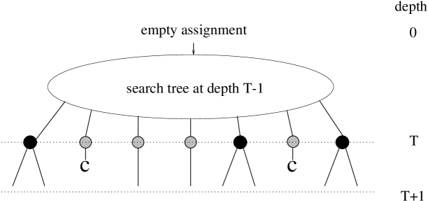
Figure 5: Imaginary, parallel growth process of an unsat search tree used in the theoretical analysis. Variables are fixed through unit-propagation, or by the splitting heuristic as in the DPLL procedure, but branches evolve in parallel. $T$ denotes the depth in the tree, that is the number of variables assigned by DPLL along each branch. At depth $T$, one literal is chosen on each branch among 1-clauses (unit-propagation, grey circles not represented on Figure 2), or 2,3-clauses (splitting, black circles as in Figure 2). If a contradiction occurs as a result of unit-propagation, the branch gets marked with C and dies out. The growth of the tree proceeds until all branches carry C leaves. The resulting tree is identical to the one built through the usual, sequential operation of DPLL.

3.2 Parallel growth process and Markovian evolution matrix

The probabilistic analysis of DPLL in the unsat regime appears to be a formidable task since the search tree of Figure 2B is the output of a complex, sequential process: nodes and edges are added by DPLL through successive descents and backtrackings (depth-first search). We have imagined a different building up of the refutation tree, which results in the same complete tree but can be mathematically analyzed. In our imaginary process (Figure 5), the tree grows in parallel, layer after layer (breadth-first search). At time $T=0$, the tree reduces to a root node, to which is attached the 3-SAT instance to be solved, and an attached outgoing edge. At time $T$, that is, after having assigned $T$ variables in the instance attached to each branch, the tree is made of $B(T)\ (\leq 2^{T})$ branches, each one carrying a partial assignment of variables. At next time step $T\to T+1$, a new layer is added by assigning, according to DPLL heuristic, one more variable along every branch. As a result, a branch may keep growing through unitary propagation, get hit by a contradiction and die out, or split if the partial assignment does not induce unit clauses. This parallel growth process is Markovian, and can be encoded in an instance–dependent matrix we now construct.

To do so, we need some preliminary definitions:

Definition 1

Partial state of variables.

The partial state $s$ of a Boolean variable $x$ is one of the three following possibilities: undetermined ($u$) if the variable has not been assigned by the search heuristic yet, true ($t$) if the variable is partially assigned to true, false ($f$) if the variable is partially assigned to false. The partial state $S$ of a set of Boolean variables $X=\{x_{1},x_{2},\ldots,x_{N}\}$ is the collection of the states of its elements, $S=\{s_{1},s_{2},\ldots,s_{N}\}$.

Let $\bf I$ be an instance of the SAT problem, defined over a set of Boolean variables $X$ with partial state $S$. A clause of $\bf I$ is said to be

• satisfied if at least one of its literals is true according to $S$;

• unsatisfied, or violated if all its literals are false according to $S$;

• undetermined otherwise; then its ‘type’ is the number $(=1,2,3)$ of undetermined variables it includes.

The instance $\bf I$ is said to be satisfied if all its clauses are satisfied, unsatisfied if one (at least) of its clauses is violated, undetermined otherwise. The set of partial states that violate ${\bf I}$ is denoted by $W$.

Definition 2

Vector space attached to a variable.

To each Boolean variable $x$ is associated a three dimensional vector space ${\bf v}$ with spanning basis $|u\rangle$, $|t\rangle$, $|f\rangle$, orthonormal with respect to the dot (inner) product denoted by $\langle.|.\rangle$,

$$\langle u|u\rangle=\langle t|t\rangle=\langle f|f\rangle=1\ ,\ \langle u|t\rangle=\langle u|f\rangle=\langle t|f\rangle=0\ .$$ (4)

The partial state attached to a basis vector $|s\rangle$ is $s$ (=$\,u,t,f)$.

Letters $u$, $t$, $f$ stand for the different partial states the variable may acquire in the course of the search process. Note that the coefficients of the decomposition of any vector $|x\rangle\in{\bf v}$ over the spanning basis,

$$|x\rangle=x^{(u)}\,|u\rangle+x^{(t)}\,|t\rangle+x^{(f)}\,|f\rangle\quad,$$ (5)

can be obtained through use of the dot product: $x^{(s)}=\langle s|x\rangle$ with $s=u,t,f$. By extension, $\langle S|$ denotes the transposed of vector $|S\rangle$.

Definition 3

Vector space attached to a set of variables.

We associate to the set $X=\{x_{1},x_{2},\ldots,x_{N}\}$ of $N$ Boolean variables the $3^{N}$–dimensional vector space ${\bf V}={\bf v}_{1}\otimes{\bf v}_{2}\otimes\ldots\otimes{\bf v}_{N}$. The spanning basis of ${\bf V}$ is the tensor product of the spanning basis of the ${\bf v}_{i}$’s. To lighten notations, we shall write $|s_{1},s_{2},...,s_{N}\rangle$ for $|s_{1}\rangle\otimes|s_{2}\rangle\otimes\ldots\otimes|s_{N}\rangle$. The partial state attached to a basis vector $|S\rangle=|s_{1},s_{2},...,s_{N}\rangle$ is $S=(s_{1},s_{2},...,s_{N})$. The dot product naturally extends over ${\bf V}$: $\langle s^{\prime}_{1},s^{\prime}_{2},\ldots,s^{\prime}_{N}|s_{1},s_{2},\ldots,s_{N}\rangle=1$ if $s_{i}=s^{\prime}_{i}\ \forall i$, 0 otherwise.

Any element $|X\rangle\in{\bf V}$ can be uniquely decomposed as a linear combination of vectors from the spanning basis. Two examples of vectors are $|\Sigma\rangle$ and $|U\rangle$, respectively the sum of all vectors in the spanning basis and the fully undetermined vector,

$$|\Sigma\rangle = \big{(}|u\rangle+|t\rangle+|f\rangle\big{)}\otimes\big{(}|u\rangle+|t\rangle+|f\rangle\big{)}\otimes\ldots\otimes\big{(}|u\rangle+|t\rangle+|f\rangle\big{)}\ ,$$ (6)

$$|U\rangle = |u,u,\ldots,u\rangle\qquad.$$ (7)

Basis vectors fulfill the closure identity

$$\sum_{S}|S\rangle\;\langle S|={\bf 1}\quad,$$ (8)

where ${\bf 1}$ is the identity operator on ${\bf V}$. To establish identity (8), apply the left hand side operator to any vector $|S^{\prime}\rangle$ and take advantage of the orthonormality of the spanning basis .

Definition 4

(Heuristic-induced) Transition probabilities

Let $S=(s_{1},s_{2},...,s_{N})$ be a partial state which does not violate instance ${\bf I}$. Call $S^{(j,x)}$, with $j=1,\ldots,N$ and $x=t,f$, the partial state obtained from $S$ by replacing $s_{j}$ with $x$. The probability that the heuristic under consideration (UC, GUC, …) chooses to assign variable $x_{j}$ when presented partial state $S$ is denoted by $h(j|S)$. The probability that the heuristic under consideration then fixes variable $x_{j}$ to $x\,(=\,t,f)$ is denoted by $g(x|S,j)$.

A few elementary facts about transition probabilities are:

1. $h(j|S)=0$ if $s_{j}\neq u$.

2. $g(x|S,j)+g(\bar{x}|S,j)=1$.

3. Assume that the number $C_{1}(S)$ of undetermined clauses of type 1 (unit clauses) is larger or equal to unity. Call $C_{1}(j|S)$ the number of unit clauses containing variable $x_{j}$, and $C_{1}(x|S,j)$ the number of unit clauses satisfied if $x_{j}$ equals $x\,(=\,t,f)$. Clearly $C_{1}(j|S)=C_{1}(t|S,j)+C_{1}(f|S,j)$. Then, as a result of unit–propagation,

   $$h(j|S) = \frac{C_{1}(j|S)}{C_{1}(S)}\quad,$$

   $$g(x|S,j) = \frac{C_{1}(x|S,j)}{C_{1}(j|S)}\quad\hbox{\rm for}\ x=t,f\ \hbox{\rm and}\ C_{1}(j|S)\geq 1\ .$$ (9)

4. In the absence of unitary clause ($C_{1}(S)=0$), transition probabilities depend on the details of the heuristic. For instance, in the case of the UC heuristic,

   1. if $s_{j}=u$, $h(j|S)=\frac{1}{u(S)}$ and $g(x|S,j)=\frac{1}{2}$,

   2. if $s_{j}\neq u$, $h(j|S)=0$,

   where $u(S)$ is the number of undetermined variables in partial state $S$.

5. The sum of transition probabilities from a partial state $S$ is equal to unity,

   $$\sum_{j=1}^{N}h(j|S)\;\bigg{[}g(t|S,j)+g(f|S,j)\bigg{]}=1\quad.$$ (10)

It is important to stress that the definition of the transition probabilities does not make any reference to any type of backtracking. It relies on the notion of variable assignement through the heuristic of search only.

Let us now introduce the

Definition 5

(Heuristic-induced) Evolution operator.

The evolution operator is a linear operator $\bf H$ acting on $\bf V$ encoding the action of DPLL for a given unsatisfiable instance ${\bf I}$. Its matrix elements in the spanning basis are

1. if $S$ violates $\bf I$,

   $$\langle S^{\prime}|{\bf H}|S\rangle=\left\{\begin{array}[]{c c}1&\hbox{\rm if}\ S^{\prime}=S\\ 0&\hbox{\rm if}\ S^{\prime}\neq S\end{array}\right.\qquad,$$ (11)

2. if $S$ does not violate $\bf I$,

   $$\langle S^{\prime}|{\bf H}|S\rangle=\left\{\begin{array}[]{c l}h(j|S)\times g(x|S,j)&\hbox{\rm if}\ C_{1}(S)\geq 1\ \hbox{\rm and}\ S^{\prime}=S^{(j,x)}\\ h(j|S)&\hbox{\rm if}\ C_{1}(S)=0\ \hbox{\rm and}\\ &\big{(}S^{\prime}=S^{(j,x)}\ \hbox{\rm or}\ S^{\prime}=S^{(j,\bar{x})}\big{)}\\ 0&\hbox{\rm otherwise}\end{array}\right.$$

where $S,S^{\prime}$ are the attached partial states to $|S\rangle,|S^{\prime}\rangle$, and $C_{1}(S)$ is the number of undetermined clauses of type 1 (unitary clauses) for partial state $S$.

Notice that we use the same notation, $\bf H$, for the operator and its matrix in the spanning basis. The different cases encountered in the above definition of $\bf H$ are symbolized in Figure 6. We may now conclude:

Theorem 6

Branch function and average size of refutation tree

Call branch function the function $B$ with integer-valued argument $T$,

$$B(T)=\langle\Sigma|{\bf H}^{T}|U\rangle\quad,$$ (12)

where $\bf H$ is the evolution operator associated to the unsatisfiable instance $\bf I$, ${\bf H}^{T}$ denotes the $T^{th}$ (matricial) power of ${\bf H}$, and vectors $|\Sigma\rangle,|U\rangle$ are defined in (6,7). Then, there exist two instance–dependent integers $T^{*}\ (\leq N)$ and $B^{*}\ (\leq 2^{N})$ such that,

$$B(T)=B^{*}\ ,\quad\forall\ T\geq T^{*}\ .$$ (13)

Furthermore, $B^{*}$ is the expectation value over the random assignments of variables of the size (number of leaves) of the search tree produced by DPLL to refute ${\bf I}$. The smallest non zero $T^{*}$ for which (13) holds is the largest number of variables that the heuristic needs to assign to reach a contradiction.

Proof of Theorem 6

Let $S$ be a partial state. We call refutation tree built from $S$ a complete search tree that proves the unsatisfiability of ${\bf I}$ conditioned to the fact that DPLL is allowed to assign only variables which are undetermined in $S$. The height of the search tree is the maximal number of assignments leading from the root node (attached to partial state $S$) to a contradictory leaf.

Let $T$ be a positive integer. We call $b_{T}(S)$ the average size (number of leaves) of refutation trees of height $\leq T$ that can be built from partial state $S$. Clearly, $b_{T}(S)=1$ for all $S\in W$, and $b_{T}(S)\geq 2$ if $S\notin W$. Recall $W$ is the set of violating partial states from Definition 1.

Assume now $T$ is an integer larger or equal to 1, $S$ a partial state with $C_{1}(S)$ unitary clauses. Our parallel representation of DPLL allows us to write simple recursion relations:

1. if $S\in W$, $b_{T}(S)=1=b_{T-1}(S)$.

2. if $S\notin W$ and $C_{1}(S)\geq 1$,

   $$b_{T}(S)=\sum_{j=1}^{N}\sum_{x=t,f}h(j|S)\,g(x|S,j)\;b_{T-1}\big{(}S^{(j,x)}\big{)}\quad.$$ (14)

3. if $S\notin W$ and $C_{1}(S)=0$,

   $$b_{T}(S)=\sum_{j=1}^{N}h(j|S)\;\bigg{[}b_{T-1}\big{(}S^{(j,t)}\big{)}+b_{T-1}\big{(}S^{(j,f)}\big{)}\bigg{]}\quad.$$ (15)

These three different cases are symbolized on Figure 6A, B and C respectively. From definitions (11,2), these recursion relations are equivalent to

$$b_{T}(S)=\sum_{S^{\prime}}\langle S^{\prime}|{\bf H}|S\rangle\;b_{T-1}(S^{\prime})\quad,$$ (16)

for any partial state $S$. Let $|b_{T}\rangle$ be the vector of $\bf V$ whose coefficients on the spanning basis $\{|S\rangle\}$ are the $b_{T}(S)$’s. In particular,

$$|b_{0}\rangle=\sum_{S_{0}\in W}|S_{0}\rangle\quad.$$ (17)

Then identity (16) can be written as $|b_{T}\rangle={\bf H}^{\dagger}\;|b_{T-1}\rangle$ where ${\bf H}^{\dagger}$ is the transposed of the evolution operator. Note that the branch function (12) is simply $B(T)=\langle U|b_{T}\rangle$. We deduce

$$|b_{T}\rangle=({\bf H}^{\dagger})^{T}\;|b_{0}\rangle=\sum_{S_{0}\in W}\sum_{\sigma_{T}}p\big{(}\sigma_{T};S_{0}\big{)}|S_{0}\rangle\quad,$$ (18)

where the second sum runs over all $3^{N\times T}$ sequences $\sigma_{T}=(S_{1},S_{2},\ldots,S_{T-1},S_{T})$ of $T$ partial states with associated weight

$$p\big{(}\sigma_{T};S_{0}\big{)} = \langle S_{T}|{\bf H}^{\dagger}|S_{T-1}\rangle\times\ldots\times\langle S_{2}|{\bf H}^{\dagger}|S_{1}\rangle\times\langle S_{1}|{\bf H}^{\dagger}|S_{0}\rangle$$ (19)

$$= \langle S_{0}|{\bf H}|S_{1}\rangle\times\langle S_{1}|{\bf H}|S_{2}\rangle\ldots\times\langle S_{T-1}|{\bf H}|S_{T}\rangle\ ,$$

The length of a sequence is the number of partial states it includes. We call $S_{0}$–genuine a sequence of partial states $\sigma_{T}$ with non zero weight (19). The second sum on the right hand side of equation (18) may be rewritten as a sum over all $S_{0}$–genuine sequences $\sigma_{T}$ of length $T$ only.

Lemma 7

Take $S_{0}\in W$. Any $S_{0}$-genuine sequence $\sigma_{N+1}$ of length $N+1$ includes at least one partial state belonging to $W$.

Suppose this is not true. There exists a genuine sequence $\sigma_{{N+1}}$ with $S_{T}\notin W$, $\forall\ 1\leq T\leq N+1$. Call $u_{T}$ the number of undetermined variables in partial state $S_{T}$. Since the sequence is genuine, $\langle S_{T-1}|{\bf H}|S_{T}\rangle\neq 0$ for every $T$ comprised between 1 and $N+1$. From the evolution operator definition (2), $S_{T}$ contains exactly one more undetermined variable than $S_{T-1}$, and $u_{T}=u_{T-1}+1$ for all $1\leq T\leq N+1$. Hence $u_{N+1}-u_{0}=N+1$. But $u_{0}$ and $u_{N+1}$ are, by definition, integer numbers comprised between 0 and $N$. ∎

From Lemma 7, the index $\nu$ of a $S_{0}$–genuine sequence $\sigma_{N+1}$ of length $N+1$,

$$\nu=\sup\big{\{}T:1\leq T\leq N+1\ \hbox{\rm and}\ S_{T}\in\sigma_{N+1}\ \hbox{\rm and}\ S_{T}\ \in\ W\big{\}}\quad,$$ (20)

exists and is larger, or equal, to $1$. Let us define

$$\hat{\sigma}_{N+1}=(S_{\nu+1},S_{\nu+2},\ldots,S_{N},S_{N+1})\quad.$$ (21)

From definition (11), $\sigma_{N+1}$ is simply $S_{0}$ repeated $\nu$ times followed by $\hat{\sigma}_{N+1}$, and $p(\sigma_{N+1})=p(\hat{\sigma}_{N+1})$. Call $\nu^{*}(S_{0})$ the smallest index of all $S_{0}$-genuine sequences of length $N+1$, and $\nu^{*}$ the minimum of $\nu^{*}(S_{0})$ over $S_{0}\in W$. Then, from equation (18), $|b_{N+1}\rangle=|b_{N}\rangle=\ldots=|b_{T^{*}}\rangle$ where $T^{*}=N+1-\nu^{*}\leq N$. Thus $|b_{T^{*}}\rangle$ is a right eigenvector of ${\bf H}^{\dagger}$ with eigenvalue unity, and $|b_{T}\rangle=|b_{T^{*}}\rangle$ for all $T\geq T^{*}$. $T^{*}$, which depends upon instance ${\bf I}$, is the length of the longest genuine sequence without repetition. It is the maximal number of (undetermined) variables to be fixed before a contradiction is found.

Lemma 8

Take $S\notin W$. Then there is no $S$-genuine sequence of length $T^{*}$.

Suppose this is not true. There exist $S\notin W$ and a $S$–genuine sequence $\sigma_{T^{*}}$ of length $T^{*}$. As $S$ does not violate ${\bf I}$, and ${\bf I}$ is not satisfiable, there are still some undetermined variables in partial state $S$. A certain number of them, say $T^{\prime}\geq 1$, must be assigned to some $t,f$ values to reach a contradiction, that is, a partial state $S_{0}\in W$. Therefore there exists a $S_{0}$–genuine sequence, $\tilde{\sigma}$, of length $T^{\prime}\geq 1$ ending with $S$ and with no repeated partial state. Concatenating $\tilde{\sigma}$ and $\sigma_{T^{*}}$, we obtain a $S_{0}$–genuine sequence of length $T^{*}+T^{\prime}>T^{*}$ and without repetition, in contradiction with the above result. ∎

Using Lemma 8, we may replace $|b_{0}\rangle$ in equation (18) with $|\Sigma\rangle$, and find

$$B(T)\equiv\langle\Sigma|{\bf H}^{T}|U\rangle=\langle U|({\bf H}^{\dagger})^{T}|\Sigma\rangle=\langle U|b_{T^{*}}\rangle=b_{T^{*}}(U)\ ,$$ (22)

for all $T\geq T^{*}$. Hence, $B^{*}=b_{T^{*}}(U)$ is the average size (over the random assignments made by the heuristic) of the refutation tree to instance $\bf I$ generated from the fully undetermined partial state. ∎

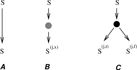
Figure 6: Transitions allowed by the heuristic-induced evolution operator. Grey and black nodes correspond to variables assigned through unit-propagation and splitting respectively, as in Figure 5. A. If the partial state $S$ already violates the instance ${\bf I}$, it is left unchanged. B. If the partial state does not violate $\bf I$ and there is at least one unitary clause, a variable is fixed through unit propagation (grey node) e.g. $x_{j}=x$. The output partial state is $S^{j,x}$. C. If the partial state does not violate $\bf I$ and there is no unitary clause, a variable $x_{j}$ is fixed through splitting (black node). Two partial states are generated, $S^{j,t}$ and $S^{j,f}$.

3.3 Some examples of short instances and associated matrices

We illustrate the above definitions and results with three explicit examples of instances involving few variables:

Example 9

Instance over $N=1$ variable

Consider the following unsat instance built from a single variable,

$${\bf I}_{1}=x_{1}\wedge\bar{x}_{1}\qquad.$$ (23)

The 3–dimensional vector space ${\bf v}_{1}$ is spanned by vectors $|u\rangle,|t\rangle,|f\rangle$. The evolution matrix reads

$${\bf H}=\left(\begin{array}[]{c c c}0&0&0\\ \frac{1}{2}&1&0\\ \frac{1}{2}&0&1\end{array}\right)\ \hbox{\rm with}\quad|u\rangle=\left(\begin{array}[]{c}1\\ 0\\ 0\end{array}\right)\ ,\quad|t\rangle=\left(\begin{array}[]{c}0\\ 1\\ 0\end{array}\right)\ ,\quad|f\rangle=\left(\begin{array}[]{c}0\\ 0\\ 1\end{array}\right)\ .$$ (24)

Entries can be interpreted as follows. Starting from the $u$ state, variable $x_{1}$ will be set through unit-propagation to $t$ or $f$ with equal probabilities: $\langle t|{\bf H}|u\rangle=\langle f|{\bf H}|u\rangle=1/2$. Once the variable has reached this state, the instance is violated: $\langle t|{\bf H}|t\rangle=\langle f|{\bf H}|f\rangle=1$. All other entries are null. In particular, state $u$ can never be reached from any state, so the first line of the matrix is filled in with zeroes: $\langle u|{\bf H}|s\rangle=0,\forall s$. Function (12) is easily calculated

$$B(T)=\left(\begin{array}[]{c}1\\ 1\\ 1\end{array}\right)^{\dagger}\;.\;{\bf H}^{T}\;.\;\left(\begin{array}[]{c}1\\ 0\\ 0\end{array}\right)=1\ ,\quad\forall\ T\geq 0\ .$$ (25)

Therefore, $T^{*}=B^{*}=1$. Indeed, refutation is obtained without any split, and the search tree involves a unique branch of length 1 (Figure 7A).

Our next example is a 2-SAT instance whose refutation requires to split one variable.

Example 10

Instance over $N=2$ variables, with a unique refutation tree.

$${\bf I}_{2}=(x_{1}\vee x_{2})\wedge(\bar{x}_{1}\vee x_{2})\wedge(x_{1}\vee\bar{x}_{2})\wedge(\bar{x}_{1}\vee\bar{x}_{2})$$ (26)

The evolution matrix $\bf H$ is a $9\times 9$ matrix with 16 non zero entries,

$$\langle s,u|{\bf H}|u,u\rangle = \langle u,s|{\bf H}|u,u\rangle=\frac{1}{2}\ ,\qquad\forall\ s=t,f$$ (27)

$$\langle s,s^{\prime}|{\bf H}|s,u\rangle = \langle s,s^{\prime}|{\bf H}|u,s^{\prime}\rangle=\frac{1}{2}\ ,\qquad\forall\ s,s^{\prime}=t,f$$ (28)

$$\langle s^{\prime},s|{\bf H}|s^{\prime},s\rangle = 1\ ,\qquad\forall\ s,s^{\prime}=t,f\quad.$$ (29)

We now explain how these matrix elements were obtained. From the undetermined state $|u,u\rangle$, any of the four clause can be chosen by the heuristic. Thus, any of the two literals $x_{1}$, $x_{2}$ has a probability $1/2$ to be chosen: $h(1|u,u)=h(2|u,u)=\frac{1}{2}$. Next, unit-propagation will set the unassigned variable to true, or false with equal probabilities $1/2$ (28). Finally, entries corresponding to violating states in eqn (29) are calculated according to rule (11).

The branch function $B(T)$ equals 1 for $T=0$, 2 for any $T\geq 1$; thus, $T^{*}=1$ and $B^{*}=2$, in agreement with the associated search tree symbolized in Figure 7B.

We now introduce an instance with a non unique refutation tree.

Example 11

Instance with $N=3$ variables, and two refutation trees.

$${\bf I}_{3}=(x_{1}\vee x_{2})\wedge(\bar{x}_{1}\vee x_{2})\wedge(x_{1}\vee\bar{x}_{2})\wedge(\bar{x}_{1}\vee\bar{x}_{2})\wedge(x_{3}\vee\bar{x}_{3})$$ (30)

Notice the presence of a (trivial) clause containing opposite literals, which allows us to obtain a variety in the search trees without considering more than three variables. The evolution matrix $\bf H$ is a $27\times 27$ matrix with 56 non zero entries (for the GUC heuristic),

$$\langle s,u,u|{\bf H}|u,u,u\rangle = \langle u,s,u|{\bf H}|u,u,u\rangle=\frac{2}{5}\ ,\qquad\forall\ s=t,f$$ (31)

$$\langle u,u,s|{\bf H}|u,u,u\rangle = \frac{1}{5}\ ,\qquad\forall\ s=t,f$$ (32)

$$\langle s,s^{\prime},s^{\prime\prime}|{\bf H}|s,u,s^{\prime\prime}\rangle = \langle s,s^{\prime},s^{\prime\prime}|{\bf H}|u,s^{\prime},s^{\prime\prime}\rangle=\frac{1}{2}\ ,\quad\forall\ s,s^{\prime}=t,f;s^{\prime\prime}=u,t,f$$

$$\langle s^{\prime},u,s|{\bf H}|u,u,s\rangle = \langle u,s^{\prime},s|{\bf H}|u,u,s\rangle=\frac{1}{2}\ ,\qquad\forall\ s,s^{\prime}=t,f$$

$$\langle s,s^{\prime},s^{\prime\prime}|{\bf H}|s,s^{\prime},s^{\prime\prime}\rangle = 1\ ,\qquad\forall\ s,s^{\prime}=t,f;\ s^{\prime\prime}=u,t,f$$

The first split variable is $x_{3}$ if the last clause is chosen (probability $1/5$), or $x_{1}$ or $x_{2}$ otherwise (with probability $2/5$ each), leading to expressions (31) and (32). The remaining entries of $\bf H$ are obtained in the same way as explained in Example 10.

We obtain $B(0)=1$, $B(1)=2$ and $B(T\geq 2)=12/5$. Therefore, $T^{*}=2$ and

$$B^{*}=\frac{12}{5}=\frac{4}{5}\times 2+\frac{1}{5}\times 4\qquad,$$ (33)

where the different contributions to $B^{*}$ and their probabilities are explicitely written down, see Figures 7B and 7C.

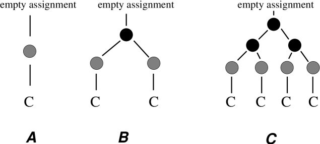
Figure 7: Refutation search trees associated to instances ${\bf I}_{1}$, ${\bf I}_{2}$ and ${\bf I}_{3}$. Grey and black nodes correspond to variables assigned through unit-propagation and split respectively, as in Figure 5. A. Example 9: refutation of instance ${\bf I}_{1}$ is obtained as a result of unit-propagation. The size (number of leaves) of the search tree is $B=1$. B. Example 10: search tree generated by DPLL on instance ${\bf I}_{2}$. The black and grey node correspond to the split of $x_{1}$ and unit-propagation over $x_{2}$, or vice-versa. The size of the tree is $B=2$. C. Example 11: search tree corresponding to the instance ${\bf I}_{3}$ when DPLL first splits variable $x_{3}$. The size of the tree is $B=4$. If the first split variable is $x_{1}$ or $x_{2}$, the refutation search tree of instance ${\bf I}_{3}$ corresponds to case B.

3.4 Dynamical annealing approximation

Let us denotes by $\overline{q}$ the expectation value of a function $q$ of the instance ${\bf I}$ over the random 3-SAT distribution, at given numbers of variable, $N$, and clauses, $\alpha\,N$. From Theorem 6, the expectation value of the size of the refutation tree is

$$B^{*}(\alpha,N)\equiv\overline{B^{*}}=\langle\Sigma|\overline{{\bf H}^{N}}|U\rangle\quad.$$ (34)

Calculation of the expectation value of the $N^{th}$ power of ${\bf H}$ is a hard task that we were unable to perform for large sizes $N$. We therefore turned to a simplifying approximation, hereafter called dynamical annealing. This approximation is not thought to be justified in general, but may be asymptotically exact in some limiting cases we will expose later on.

A first temptation is to approximate the expectation of the $N^{th}$ power of ${\bf H}$ with the $N^{th}$ power of the expectation of ${\bf H}$. This is however too a brutal approximation to be meaningful, and a more refined scheme is needed.

Definition 12

Clause projection operator

Consider an instance ${\bf I}$ of the 3-SAT problem. The clause vector $\vec{C}(S)$ of a partial state $S$ is a three dimensional vector $\vec{C}=(C_{1},C_{2},C_{3})$ where $C_{j}$ is the number of undetermined clauses of ${\bf I}$ of type $j$. The clause projection operator, ${\bf P}({\vec{C}})$, is the operator acting on $\bf V$ and projecting onto the subspace of partial state vectors with clause vectors $\vec{C}$,

$${\bf P}({\vec{C}})\;|S\rangle=\left[\prod_{j=1}^{3}\delta_{C_{j}-C_{j}(S)}\right]\ |S\rangle\quad,$$ (35)

where $\delta$ is the Kronecker function. The sum of all state vectors in the spanning basis with clause vector $\vec{C}$ is denoted by $|\Sigma(\vec{C})\rangle={\bf P}({\vec{C}})\;|\Sigma\rangle$. The sum of all state vectors in the spanning basis with clause vector $\vec{C}$ and $U$ undetermined variables is denoted by $|\Sigma_{U}(\vec{C})\rangle$.

It is an easy check that ${\bf P}$ is indeed a projection operator: ${\bf P}^{2}({\vec{C}})={\bf P}({\vec{C}})$. As the set of partial states can be partitioned according to their clause vectors,

$$\sum_{\vec{C}}{\bf P}({\vec{C}})=\sum_{\vec{C}}{\bf P}^{2}({\vec{C}})={\bf 1}\quad.$$ (36)

We now introduce the clause vector-dependent branch function

$$B(\vec{C},T)=\langle\Sigma(\vec{C})|{\bf H}^{T}|U\rangle\quad.$$ (37)

Summation of the $B$’s over all $\vec{C}$ gives back function (12) from identity (36). The evolution equation for $B(\vec{C},T)$ is,

$$B(\vec{C},T+1) = \langle\Sigma(\vec{C})|{\bf H}\;\times{\bf H}^{T}|U\rangle$$ (38)

$$= \langle\Sigma(\vec{C})|{\bf H}\times\left(\sum_{\vec{C}^{\prime}}{\bf P}^{2}({\vec{C}^{\prime}})\right)\times{\bf H}^{T}|U\rangle$$

$$= \sum_{\vec{C}^{\prime}}\;\langle\Sigma(\vec{C})|{\bf H}\times{\bf P}({\vec{C}^{\prime}})\times\left(\sum_{S}|S\rangle\langle S|\right)\times{\bf P}({\vec{C}^{\prime}})\times{\bf H}^{T}|U\rangle$$

$$= \sum_{\vec{C}^{\prime}}\sum_{S}\langle\Sigma(\vec{C})|{\bf H}\times{\bf P}({\vec{C}^{\prime}})|S\rangle\;\langle S|{\bf P}({\vec{C}^{\prime}})\times{\bf H}^{T}|U\rangle$$

where we have made use of identities (8) and (36). We are now ready to do the two following approximation steps:

Approximation 13

Dynamical annealing (step A)

Substitute in equation (38) the partial state vector

$${\bf P}(\vec{C}^{\prime})\,|S\rangle\quad\hbox{ with}\quad\frac{1}{\langle\Sigma|\Sigma_{N-T}(\vec{C}^{\prime})\rangle}\;|\Sigma_{N-T}(\vec{C}^{\prime})\rangle\quad,$$ (39)

that is, with its average over the set of basis vectors with clause vector $\vec{C}^{\prime}$ and $N-T$ undetermined variables.

Following step A, equation (38) becomes an approximated evolution equation for $B$,

$$B(\vec{C},T+1)=\sum_{\vec{C}^{\prime}}{\bf\hat{H}}[\vec{C},\vec{C}^{\prime};T]\;B(\vec{C},T)\quad,$$ (40)

where the new evolution matrix ${\bf\hat{H}}$, not to be confused with ${\bf H}$, is

$${\bf\hat{H}}[\vec{C},\vec{C}^{\prime};T]=\frac{\langle\Sigma(\vec{C})|{\bf H}|\Sigma_{N-T}(\vec{C}^{\prime})\rangle}{\langle\Sigma|\Sigma_{N-T}(\vec{C}^{\prime})\rangle}\quad.$$ (41)

Then,

Approximation 14

Dynamical annealing (step B)

Substitute in equation (40) the evolution matrix ${\bf\hat{H}}$ with

$${\bf\bar{H}}[\vec{C},\vec{C}^{\prime};T]=\frac{\overline{\langle\Sigma(\vec{C})|{\bf H}|\Sigma_{N-T}(\vec{C}^{\prime})\rangle}}{\overline{\langle\Sigma|\Sigma_{N-T}(\vec{C}^{\prime})\rangle}}$$ (42)

that is, consider the instance ${\bf I}$ is redrawn at each time step $T\to T+1$, keeping information about clause vectors at time $T$ only.

Let us interpret what we have done so far. The quantity we focus on is $\bar{B}(\vec{C};T+1)$, the expectation number of branches at depth $T$ in the search tree (Figure 5) carrying partial states with clause vector $\vec{C}=(C_{1},C_{2},C_{3})$. Within the dynamical annealing approximation, the evolution of the $\bar{B}$’s is Markovian,

$$\bar{B}(\vec{C};T+1)=\sum_{\vec{C}^{\prime}}\;{\bf\bar{H}}\;[\vec{C},\vec{C}^{\prime};T]\;\bar{B}(\vec{C}^{\prime};T)\ .$$ (43)

The entries of the evolution matrix ${\bf\bar{H}}[\vec{C},\vec{C}^{\prime};T]$ can be interpreted as the average number of branches with clause vector $\vec{C}$ that DPLL will generate through the assignment of one variable from a partial assignment (partial state) of variables with clause vector $\vec{C}^{\prime}$.

For the GUC heuristic, we find (Cocco and Monasson, 2001),

$${\bf\bar{H}}[\vec{C},\vec{C}^{\prime};T]={C_{3}^{\prime}\choose C_{3}^{\prime}-C_{3}}\;\left(\frac{3}{N-T}\right)^{C_{3}^{\prime}-C_{3}}\;\left(1-\frac{3}{N-T}\right)^{C_{3}}\times$$

$$\qquad\qquad\qquad\qquad\sum_{w_{2}=0}^{C_{3}^{\prime}-C_{3}}\left(\frac{1}{2}\right)^{C_{3}^{\prime}-C_{3}}{C_{3}^{\prime}-C_{3}\choose w_{2}}\times$$

$$\left\{(1-\delta_{C^{\prime}_{1}})\;\left(1-\frac{1}{2(N-T)}\right)^{C^{\prime}_{1}-1}\sum_{z_{2}=0}^{C_{2}^{\prime}}{C_{2}^{\prime}\choose z_{2}}\left(\frac{2}{N-T}\right)^{z_{2}}\right.\times$$

$$\left(1-\frac{2}{N-T}\right)^{C_{2}^{\prime}-z_{2}}\sum_{w_{1}=0}^{z_{2}}\left(\frac{1}{2}\right)^{z_{2}}{z_{2}\choose w_{1}}\;\delta_{C_{2}-C_{2}^{\prime}-w_{2}+z_{2}}\;\delta_{C_{1}-C_{1}^{\prime}-w_{1}+1}+$$

$$\delta_{C_{1}^{\prime}}\sum_{z_{2}=0}^{C_{2}^{\prime}-1}{C_{2}^{\prime}-1\choose z_{2}}\left(\frac{2}{N-T}\right)^{z_{2}}\,\left(1-\frac{2}{N-T}\right)^{C_{2}^{\prime}-1-z_{2}}\times$$

$$\left.\sum_{w_{1}=0}^{z_{2}}\left(\frac{1}{2}\right)^{z_{2}}{z_{2}\choose w_{1}}\;\delta_{C_{2}-C_{2}^{\prime}-w_{2}+z_{2}+1}\;[\delta_{C_{1}-w_{1}}+\delta_{C_{1}-1-w_{1}}]\right\}\ ,$$ (44)

where $\delta_{X}$ denotes the Kronecker delta function over integers $X$: $\delta_{X}=1$ if $X=0$, $\delta_{X}=0$ otherwise. Expression (3.4) is easy to obtain from the interpretation following equation (43).

3.5 Generating functions and asymptotic scalings at large $N$

Let us introduce the generating function $G(\,{\vec{y}}\,;T\,)$ of the average number of branches $\bar{B}(\,{\vec{C}}\,;T\,)$ where $\vec{y}\equiv(y_{1},y_{2},y_{3})$, through

$$G(\,{\vec{y}}\,;T\,)=\sum_{\vec{C}}\;e^{\,{\vec{y}}\cdot{\vec{C}}}\;\bar{B}(\,{\vec{C}}\,,T\,)\quad,\quad{\vec{y}}\cdot{\vec{C}}\equiv\sum_{j=1}^{3}y_{j}\,C_{j}\quad.$$ (45)

Evolution equation (40) for the $\bar{B}$’s can be rewritten in term of the generating function $G$,

$$G(\,{\vec{y}}\,;T+1\,) = e^{-\gamma_{1}({\vec{y}})}\;G\big{(}\,{\vec{\gamma}}({\vec{y}})\,;T\,\big{)}+$$ (46)

$$\left(e^{-\gamma_{2}({\vec{y}})}(e^{y_{1}}+1)-e^{-\gamma_{1}({\vec{y}})}\right)\;G\big{(}-\infty,\,\gamma_{2}({\vec{y}}),\,\gamma_{3}({\vec{y}})\,;T\,\big{)}$$

where ${\vec{\gamma}}$ is a vectorial function of argument ${\vec{y}}$ whose components read

$$\gamma_{1}({\vec{y}}) = y_{1}+\ln\left[1-\frac{1}{2(N-T)}\right]\quad,$$

$$\gamma_{2}({\vec{y}}) = y_{2}+\ln\left[1+\frac{2}{N-T}\left(\frac{e^{-y_{2}}}{2}\left(1+e^{y_{1}}\right)-1\right)\right]\quad,$$

$$\gamma_{3}({\vec{y}}) = y_{3}+\ln\left[1+\frac{3}{N-T}\left(\frac{e^{-y_{3}}}{2}\left(1+e^{y_{2}}\right)-1\right)\right]\quad.$$ (47)

To solve equation (46), we infer the large $N$ behaviour of $G$ from the following remarks:

1. Each time DPLL assigns variables through splitting or unit-propagation, the numbers $C_{j}$ of clauses of length $j$ undergo $O(1)$ changes. It is thus sensible to assume that, when the number of assigned variables increases from $T_{1}=t\,N$ to $T_{2}=t\,N+\Delta T$ with $\Delta T$ very large but $o(N)$ e.g. $\Delta T=\sqrt{N}$, the densities $c_{2}=C_{2}/N$ and $c_{3}=C_{3}/N$ of 2- and 3-clauses have been modified by $o(1)$.

2. On the same time interval $T_{1}<T<T_{2}$, we expect the number of unit-clauses $C_{1}$ to vary at each time step. But its distribution $\rho(C_{1}|c_{2},c_{3};t)$, conditioned to the densities $c_{2}$, $c_{3}$ and the reduced time $t$, should reach some well defined limit distribution. This claim is a generalization of the result obtained by Frieze and Suen (1996) for the analysis of the GUC heuristic in the absence of backtracking.

3. As long as a partial state does not violate the instance, very few unit-clauses are generated, and splitting frequently occurs. In other words, the probability that $C_{1}=0$ is strictly positive as $N$ gets large.

The above arguments entice us to make the following

Claim 15

Asymptotic expression for the generating function $G$

For large $N,T$ at fixed ratio $t=T/N$, the generating function (45) of the average numbers $\bar{B}$ of branches is expected to behave as

$$G(y_{1},y_{2},y_{3};t\,N)=\exp\bigg{[}\,N\,\varphi(y_{2},y_{3};t)+\psi(y_{1},y_{2},y_{3};t)+o(1)\bigg{]}\quad.$$ (48)

Hypothesis (48) expresses in a concise way some important information on the distribution of clause populations during the search process that we now extract. Call $\omega$ the Legendre transform of $\varphi$,

$$\omega(\,c_{2},c_{3}\,;t\,)=\min_{y_{2},y_{3}}\bigg{[}\varphi(\,y_{2},y_{3}\,;t\,)-y_{2}\,c_{2}-y_{3}\,c_{3}\bigg{]}\qquad.$$ (49)

Then, combining equations (45), (48) and (49), we obtain

$$\sum_{C_{1}\geq 0}\rho(C_{1}|c_{2},c_{3};t)\;\bar{B}(C_{1},c_{2}\,N,c_{3}\,N;t\,N)\asymp\exp\big{[}\,N\,\omega(c_{2},c_{3};t\,)\big{]}\quad,$$ (50)

up to non exponential in $N$ corrections. In other words, the expectation value of the number of branches carrying partial states with $(1-t)\,N$ undetermined variables and $c_{j}\,N$ $j$-clauses ($j=2,3$) scales exponentially with $N$, with a growth function $\omega(c_{2},c_{3};t)$ related to $\varphi(y_{2},y_{3};t)$ through identity (49). Moreover, $\varphi(0,0;t)$ is the logarithm of the number of branches (divided by $N$) after a fraction $t$ of variables have been assigned. The most probable values of the densities $c_{j}(t)$ of $j$-clauses are then obtained from the partial derivatives of $\varphi$: $c_{j}(t)=\partial\varphi/\partial y_{j}(0,0)$ for $j=2,3$.

Let us emphasize that $\varphi$ in equation (48) does not depend on $y_{1}$. This hypothesis simply expresses that, as far as non violating partial states are concerned, both terms on the right hand side of (46) are of the same order, and that the density of unit-clauses, $c_{1}=\partial\varphi/\partial y_{1}$, identically vanishes.

Similarly, function $\psi(y_{1},y_{2},y_{3};t)$ is related to the generating function of distribution $\rho(C_{1}|c_{2},c_{3};t)$,

$$\sum_{C_{1}\geq 0}\rho(C_{1}|c_{2},c_{3};t)\,\e^{y_{1}\,C_{1}}=e^{\psi(y_{1},y_{2},y_{3};t)-\psi(0,y_{2},y_{3};t)}\quad,$$ (51)

where $c_{j}=\partial\varphi/\partial y_{j}(y_{2},y_{3};t)$ ($j=2,3$) on the left hand side of the above formula.

Inserting expression (48) into the evolution equation (46), we find

$$\frac{\partial\varphi}{\partial t}(y_{2},y_{3};t) = -y_{1}+\frac{2}{1-t}\left[e^{-y_{2}}\left(\frac{1+e^{y_{1}}}{2}\right)-1\right]\frac{\partial\varphi}{\partial y_{2}}(y_{2},y_{3};t)$$ (52)

$$+ \frac{3}{1-t}\left[e^{-y_{3}}\left(\frac{1+e^{y_{2}}}{2}\right)-1\right]\frac{\partial\varphi}{\partial y_{3}}(y_{2},y_{3};t)$$

$$+ \ln\left[1+K(y_{1},y_{2})\;e^{\psi(-\infty,y_{2},y_{3};t)-\psi(y_{1},y_{2},y_{3};t)}\right]$$

where $K(y_{1},y_{2})=e^{-y_{2}}(e^{2\,y_{1}}+e^{y_{1}})-1$. As $\varphi$ does not depend upon $y_{1}$, the latter may be chosen at our convenience e.g. to cancel $K$ and the contribution from the last term in equation (52),

$$y_{1}=Y_{1}(y_{2})\equiv y_{2}-\ln\left(\frac{1+\sqrt{1+4e^{y_{2}}}}{2}\right)\quad.$$ (53)

Such a procedure, sometimes called kernel method and, to our knowledge, first proposed by Knuth (1968), is correct in the major part of the $y_{2},y_{3}$ space and, in particular, in the vicinity of $(0,0)$ we focus on in this paper. We end up with the following partial differential equation (PDE) for $\varphi$,

$$\frac{\partial\varphi}{\partial t}(y_{2},y_{3};t)={H}\left[\frac{\partial\varphi}{\partial y_{2}},\frac{\partial\varphi}{\partial y_{3}},y_{2},y_{3},t\right]\quad,$$ (54)

where ${H}$ incorporates the details of the splitting heuristic,

$${H}_{GUC}[c_{2},c_{3},y_{2},y_{3},t] = -Y_{1}(y_{2})+\frac{3\,c_{3}}{1-t}\;\left[e^{-y_{3}}\;\left(\frac{1+e^{y_{2}}}{2}\right)-1\right]$$ (56)

$$+ \frac{c_{2}}{1-t}\;\left(e^{-Y_{1}(y_{2})}-2\right)\qquad.$$

We must therefore solve the partial differential equation (PDE) (54) with the initial condition,

$$\varphi(y_{2},y_{3},t=0)=\alpha_{0}\;y_{3}\quad,$$ (57)

obtained through inverse Legendre transform (49) of the initial condition over $\bar{B}$, or equivalently over $\omega$,

$$\omega(c_{2},c_{3};t=0)=\left\{\begin{array}[]{c c c}0&\hbox{\rm if}&c_{3}=\alpha_{0}\ ,\\ -\infty&\hbox{\rm if}&c_{3}\neq\alpha_{0}\ .\end{array}\right.$$

${}^{\ }$                          

Figure 8: Snapshots of the surface $\omega(p,\alpha;t)$ for $\alpha_{0}=10$ at three different times i.e. depths in the tree, $t=0.01$, 0.05 and 0.09 (from left to right, top to down). The height $\omega^{*}(t)$ of the top of the surface, with coordinates $p^{*}(t),\alpha^{*}(t)$, is the logarithm (divided by $N$) of the number of branches. The coordinates $(p^{*}(t),\alpha^{*}(t))$ define the tree trajectory shown in Figure 3. The halt line is hit at $t_{h}\simeq 0.094$. Note the overall growth of the surface $\omega(p,\alpha;t)$ with time (beware of the change of scales between figures).

3.6 Interpretation in terms of growth process

We can interpret the dynamical annealing approximation made in the previous paragraphs, and the resulting PDE (54) as a description of the growth process of the search tree resulting from DPLL operation. Using Legendre transform (49), PDE (54) can be written as an evolution equation for the logarithm $\omega(c_{2},c_{3},t)$ of the average number of branches with parameters $c_{2},c_{3}$ as the depth $t=T/N$ increases,

$$\frac{\partial\omega}{\partial t}(c_{2},c_{3},t)={H}\left[c_{2},c_{3},-\frac{\partial\omega}{\partial c_{2}},-\frac{\partial\omega}{\partial c_{3}},t\right]\qquad.$$ (58)

Partial differential equation (PDE) (58) is analogous to growth processes encountered in statistical physics (McKane, Droz, Vannimenus and Wolf, 1995). The surface $\omega$, growing with “time” $t$ above the plane $c_{2},c_{3}$, or equivalently from (3), above the plane $p,\alpha$ (Figure 8), describes the whole distribution of branches. The average number of branches at depth $t$ in the tree equals

$$B(t)=\int_{0}^{1}dp\;\int_{0}d\alpha\;e^{N\,\omega(p,\alpha;t)}\asymp e^{N\,\omega^{*}(t)}\quad,$$ (59)

where $\omega^{*}(t)$ is the maximum over $p,\alpha$ of $\omega(p,\alpha;t)$ reached in $p^{*}(t),\alpha^{*}(t)$. In other words, the exponentially dominant contribution to $B(t)$ comes from branches carrying 2+p-SAT instances with parameters $p^{*}(t),\alpha^{*}(t)$, that is clause densities $c^{*}_{2}(t)=\alpha^{*}(t)(1-p^{*}(t))$, $c^{*}_{3}(t)=\alpha^{*}(t)p^{*}(t)$. Parametric plot of $p^{*}(t),\alpha^{*}(t)$ as a function of $t$ defines the tree trajectories on Figure 3.

The hyperbolic line in Figure 3 indicates the halt points, where contradictions prevent dominant branches from further growing. Each time DPLL assigns a variable through unit-propagation, an average number $u(p,\alpha)$ of new 1-clauses is produced, resulting in a net rate of $u-1$ additional 1-clauses. As long as $u<1$, 1-clauses are quickly eliminated and do not accumulate. Conversely, if $u>1$, 1-clauses tend to accumulate. Opposite 1-clauses $x$ and $\bar{x}$ are likely to appear, leading to a contradiction (Chao and Franco, 1990; Frieze and Suen, 1996). The halt line is defined through $u(p,\alpha)=1$, and reads (Cocco and Monasson, 2001),

$$\alpha=\left(\frac{3+\sqrt{5}}{2}\right)\ln\left[\frac{1+\sqrt{5}}{2}\right]\;\frac{1}{1-p}\qquad.$$ (60)

It differs from the halt line $\alpha=1/(1-p)$ corresponding to a single branch (Frieze and Suen, 1996). As far as dominant branches are concerned, an alternative and simpler way of obtaining the halt criterion is through calculation of the probability $\rho^{*}_{S}(t)\equiv\rho(C_{1}=0|c^{*}_{2}(t),c^{*}_{3}(t);t)$ that a split occurs when a variable is assigned by DPLL,

$$\rho^{*}_{S}(t)=\exp\left(\frac{\partial\varphi}{\partial t}(0,0;t)\right)-1\quad,$$ (61)

from equations (51,52). The probability of split vanishes, and unit-clauses accumulate till a contradiction is obtained, when the tree stops growing. Along the tree trajectory, $\omega^{*}(t)$ grows thus from 0, on the right vertical axis, up to some final positive value, $\omega_{THE}$, on the halt line. $\omega_{THE}$ is our theoretical prediction for the logarithm of the complexity (divided by $N$).

Equation (58) was solved using the method of characteristics. Using eqn. (3), we have plotted the surface $\omega$ at different times, with the results shown in Figure 8 for $\alpha_{0}=10$. Values of $\omega_{THE}$, obtained for $4.3<\alpha<20$ by solving equation (58) compare very well with numerical results (Table 1). We stress that, though our calculation is not rigorous, it provides a very good quantitative estimate of the complexity. It is therefore expected that our dynamical annealing approximation be quantitavely accurate. It is a reasonable conjecture that it becomes exact at large ratios $\alpha_{0}$, where PDE (54) can be exactly solved:

Conjecture 16

Asymptotic equivalent of $\omega$ for large ratios

Resolution of PDE (58) in the large ratio $\alpha_{0}$ limit gives (for the GUC heuristic),

$$\omega_{THE}(\alpha_{0})\asymp\frac{3+\sqrt{5}}{6\,\ln 2}\;\left[\ln\left(\frac{1+\sqrt{5}}{2}\right)\right]^{2}\;\frac{1}{\alpha_{0}}\quad.$$ (62)

This result exhibits the $1/\alpha_{0}$ scaling proven by Beame et al. (1998), and is conjectured to be exact.

As $\alpha_{0}$ increases, search trees become smaller and smaller, and correlations between branches, weaker and weaker, making dynamical annealing more and more accurate.

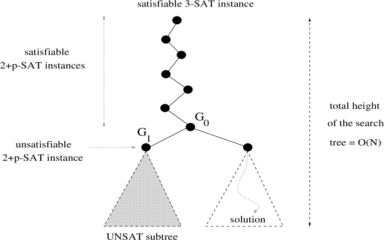
Figure 9: Detailed structure of the search tree in the upper sat phase ($\alpha_{L}<\alpha<\alpha_{C}$). DPLL starts with a satisfiable 3-SAT instance and transforms it into a sequence of 2+p-SAT instances. The leftmost branch in the tree symbolizes the first descent made by DPLL. Above node $G_{0}$, instances are satisfiable while below $G_{1}$, instances have no solutions. A grey triangle accounts for the (exponentially) large refutation subtree that DPLL has to go through before backtracking above $G_{1}$ and reaching $G_{0}$. By definition, the highest node reached back by DPLL is $G_{0}$. Further backtracking, below $G_{0}$, will be necessary but a solution will be eventually found (right subtree), see Figure 2C.

4 Upper phase and mixed branch–tree trajectories.

The interest of the trajectory framework proposed in this paper is best seen in the upper sat phase, that is, for ratios $\alpha_{0}$ ranging from $\alpha_{L}$ to $\alpha_{C}$. This intermediate region juxtaposes branch and tree behaviors, see search tree in Figures 2C and 9.

The branch trajectory, started from the point $(p=1,\alpha_{0})$ corresponding to the initial 3-SAT instance, hits the critical line $\alpha_{c}(p)$ at some point G with coordinates ($p_{G},\alpha_{G}$) after $N\;t_{G}$ variables have been assigned by DPLL, see Figure 3. The algorithm then enters the unsat phase and, with high probability, generates a 2+p-SAT instance with no solution. A dense subtree that DPLL has to go through entirely, forms beyond G till the halt line (left subtree in Figure 9). The size of this subtree can be analytically predicted from the theory exposed in Section 3. All calculations are identical, except initial condition (57) which has to be changed into

$$\varphi(y_{2},y_{3},t=0)=\alpha_{G}\;(1-p_{G})\;y_{2}+\alpha_{G}\;p_{G}\;y_{3}\quad.$$ (63)

As a result we obtain the size $2^{N_{G}\;\omega_{G}}$ of the unsatisfiable subtree to be backtracked (leftmost subtree in Figure 9). $N_{G}=N\,(1-t_{G})$ denotes the number of undetermined variables at point $G$.

$G$ is the highest backtracking node in the tree (Figures 2C and 9) reached back by DPLL, since nodes above G are located in the sat phase and carry 2+p-SAT instances with solutions. DPLL will eventually reach a solution. The corresponding branch (rightmost path in Figure 2C) is highly non typical and does not contribute to the complexity, since almost all branches in the search tree are described by the tree trajectory issued from G (Figure 3). We expect that the computational effort DPLL requires to find a solution will, to exponential order in $N$, be given by the size of the left unsatisfiable subtree of Figure 9. In other words, massive backtracking will certainly be present in the right subtree (the one leading to the solution), and no significant statistical difference is expected between both subtrees.

We have experimentally checked this scenario for $\alpha_{0}=3.5$. The average coordinates of the highest backtracking node, $(p_{G}\simeq 0.78,\alpha_{G}\simeq 3.02$), coincide with the computed intersection of the single branch trajectory (Section 2.2) and the estimated critical line $\alpha_{c}(p)$ (Cocco and Monasson, 2001). As for complexity, experimental measures of $\omega$ from 3-SAT instances at $\alpha_{0}=3.5$, and of $\omega_{G}$ from 2+0.78-SAT instances at $\alpha_{G}=3.02$, obey the expected identity

$$\omega_{THE}=\omega_{G}\times(1-t_{G})\quad,$$ (64)

and are in very good agreement with theory (Table 1). Therefore, the structure of search trees corresponding to instances of 3-SAT in the upper sat regime reflects the existence of a critical line for 2+p-SAT instances.

5 Conclusions.

In this paper, we have exposed a procedure to understand the complexity pattern of the backtrack resolution of the random Satisfiability problem (Figure 10). Main steps are:

1. Identify the space of parameters in which the dynamical evolution takes place; this space will be generally larger than the initial parameter space since the algorithm modifies the instance structure. While the distribution of 3-SAT instances is characterized by the clause per variable ratio $\alpha$ only, another parameter $p$ accounting for the emergence of 2-clauses has to be considered.

2. Divide the parameter space into different regions (phases) depending on the output of the resolution e.g. sat/unsat phases for 2+p-SAT.

3. Represent the action of the algorithm as trajectories in this phase diagram. Intersection of trajectories with the phase boundaries allow to distinguish hard from easy regimes (Figure 10).

In addition, we have also presented a non rigorous study of the search tree growth, which allows us to accurately estimate the complexity of resolution in presence of massive backtracking. From a mathematical point of view, it is worth noticing that monitoring the growth of the search tree requires a PDE, while ODEs are sufficient to account for the evolution of a single branch (Achlioptas, 2001b).

An interesting question raised by this picture is the robustness of the polynomial/exponential crossover point T (Figure 3). While the ratio $\alpha_{L}$ separating easy (polynomial) from hard (exponential) resolutions depends on the heuristics used by DPLL ($\alpha_{L}^{GUC}\simeq 3.003$, $\alpha_{L}^{UC}=8/3$), T appears to be located at the same coordinates $(p_{T}=2/5,\alpha_{T}=5/3)$ for all three UC, GUC, and SC₁ heuristics. From a technical point of view, the robustness of T comes from the structure of the ODEs (2). The coordinates of T, and the time $t_{T}$ at which the branch trajectory issued from $(p=1,\alpha_{0}=\alpha_{L})$ hits the critical line $\alpha_{C}(p)$ tangentially, obey the equations $\rho_{1}=\partial\rho_{1}/\partial t=0$ with $\rho_{1}=1-\alpha(t)\big{(}1-p(t)\big{)}$. The set of ODEs (2), combined with the previous conditions, gives $p_{T}=2/5$ (Achlioptas, 2001b).

This robustness explains why the polynomial/exponential crossover location of critically constrained 2+p-SAT instances, which should a priori depend on the algorithm used, was found by Monasson et al. (1999) to coincide roughly with the algorithm–independent, tricritical point on the $\alpha_{C}(p)$ line.

Our approach has already been extended to other decision problems, e.g. the vertex covering of random graphs (Hartmann and Weigt, 2001) or the coloring of random graphs (Ein-Dor and Monasson, 2003) (see (Jia and Moore, 2003) for recent rigorous results on backtracking in this case). It is important to stress that it is not limited to the determination of the average solving time, but may also be used to capture its distribution (Gent and Walsh, 1994; Cocco and Monasson, 2002; Montanari and Zecchina, 2002) and to understand the efficiency of restarts techniques (Gomes et al., 2000). Finally, we emphasize that theorem 6 relates the computational effort to the evolution operator representing the elementary steps of the search heuristic for a given instance. It is expected that this approach will be useful to obtain results on the average-case complexity of DPLL at fixed instance, where the average is performed over the random choices done by the algorithm only (Monasson, 2003).

Figure 10: Schematic representation of the resolution trajectories in the sat (branch trajectories symbolized with dashed line) and unsat (tree trajectories represented by hatched regions) phases. DPLL goes along branch trajectories in a linear time, but takes an exponential time to go through tree trajectories. The mixed case of hard sat instances correspond to the crossing of the boundary separating the two phases (bold line), which leads to the exploration of unsat subtrees before a solution is finally found.

References

- (1)
- Achlioptas et al. (2001a) Achlioptas, D., Kirousis, L., Kranakis, E. and Krizanc, D. Rigorous results for random (2+p)-SAT, Theor. Comp. Sci. 265, 109-129 (2001).
- Achlioptas (2001b) Achlioptas, D. Lower bounds for random 3-SAT via differential equations, Theor. Comp. Sci. 265, 159–185 (2001).
- Achlioptas, Beame and Molloy (2001c) Achlioptas, D., Beame, P. and Molloy, M. A Sharp Threshold in Proof Complexity. in Proceedings of STOC 01, p.337-346 (2001).
- Beame et al. (1998) Beame, P., Karp, R., Pitassi, T. and Saks, M. ACM Symp. on Theory of Computing (STOC98), 561–571 Assoc. Comput. Mach., New York (1998).
- Chao and Franco (1986) Chao, M.T. and Franco, J. Probabilistic analysis of two heuristics for the 3-satisfiability problem, SIAM Journal on Computing 15, 1106-1118 (1986).
- Chao and Franco (1990) Chao, M.T. and Franco, J. Probabilistic analysis of a generalization of the unit-clause literal selection heuristics for the k-satisfiability problem, Information Science 51, 289–314 (1990).
- Chvàtal and Szmeredi (1988) Chvàtal, V. and Szmeredi, E. Many hard examples for resolution, Journal of the ACM 35, 759–768 (1988).
- Coarfa et al. (2000) Coarfa, C., Dernopoulos, D.D., San Miguel Aguirre, A., Subramanian, D. and Vardi, M.Y. Random 3-SAT: The plot thickens. In R. Dechter, editor, Proc. Principles and Practice of Constraint Programming (CP’2000), Lecture Notes in Computer Science 1894, 143-159 (2000).
- Cocco and Monasson (2001) Cocco, S. and Monasson, R. Trajectories in phase diagrams, growth processes and computational complexity: how search algorithms solve the 3-Satisfiability problem, Phys. Rev. Lett. 86, 1654 (2001); Analysis of the computational complexity of solving random satisfiability problems using branch and bound search algorithms, Eur. Phys. J. B 22, 505 (2001).
- Cocco and Monasson (2002) Cocco, S. and Monasson R. Exponentially hard problems are sometimes polynomial, a large deviation analysis of search algorithms for the random satisfiability problem, and its application to stop-and-restart resolutions, Phys. Rev. E 66, 037101 (2002).
- Crawford and Auton (1996) Crawford, J. and Auton, L. Experimental Results on the Cross-Over Point in Satisfiability Problems, Proc. 11th Natl. Conference on Artificial Intelligence (AAAI-93), 21–27, The AAAI Press / MIT Press, Cambridge, MA (1993); Artificial Intelligence 81 (1996).
- Davis, Logemann and Loveland (1962) Davis, M., Logemann, G., Loveland, D. A machine program for theorem proving. Communications of the ACM 5, 394-397 (1962).
- Dubois, Boufkhad and Mandler (2000) Dubois, O., Boufkhad, Y. and Mandler, J. Typical random 3-SAT formulae and the satisfiability threshold. SODA, p. 126-127 (2000).
- Dubois et al. (2001) Dubois, O., Monasson, R., Selman, B. and Zecchina, R. (eds) Phase transitions in combinatorial problems. Theor. Comp. Sci. 265 (2001).
- Franco (2001) Franco, J. Results related to thresholds phenomena research in satisfiability: lower bounds. Theor. Comp. Sci. 265, 147–157 (2001).
- Friedgut (1999) Friedgut, E. Sharp thresholds of graph properties, and the k-sat problem, Journal of the A.M.S. 12, 1017 (1999).
- Frieze and Suen (1996) Frieze, A. and Suen, S. Analysis of two simple heuristics on a random instance of k-SAT, Journal of Algorithms 20, 312–335 (1996).
- Gent and Walsh (1994) Gent, I.P. and Walsh, T. Easy problems are sometimes hard, Artificial Intelligence 70, 335-345 (1994).
- Gent, van Maaren and Walsh (2000) Gent , I., van Maaren, H. and Walsh, T. (eds). SAT2000: Highlights of Satisfiability Research in the Year 2000, Frontiers in Artificial Intelligence and Applications, vol. 63, IOS Press, Amsterdam (2000).
- Gomes et al. (2000) Gomes, C.P., Selman, B., Crato, N. and Kautz, H. J. Automated Reasoning 24, 67 (2000).
- Gu, Purdom, Franco and Wah (1997) Gu, J., Purdom, P.W., Franco, J. and Wah, B.W. Algorithms for satisfiability (SAT) problem: a survey. DIMACS Series on Discrete Mathematics and Theoretical Computer Science 35, 19-151, American Mathematical Society (1997).
- Hartmann and Weigt (2001) Hartmann, A. and Weigt, M. Typical solution time for a vertex-covering algorithm on finite-connectivity random graphs, Phys. Rev. Lett. 86, 1658 (2001).
- Hogg, Huberman and Williams (1996) Hogg, T., Huberman, B.A. and Williams, C. (eds). Frontiers in problem solving: phase transitions and complexity. Artificial Intelligence 81 I & II (1996).
- Jia and Moore (2003) Jia, H. and Moore, C. How much backtracking does it take to 3-color a random graph? preprint (2003).
- Kaporis, Kirousis and Lalas (2002) Kaporis, A.C., Kirousis, L.M. and Lalas, E.G. The Probabilistic Analysis of a Greedy Satisfiability Algorithm. ESA, p. 574-585 (2002).
- Knuth (1968) Knuth, D.E. The art of computer programming, vol. 1: Fundamental algorithms, Section 2.2.1, Addison-Wesley, New York (1968).
- Ein-Dor and Monasson (2003) Ein-Dor, L. and Monasson, R. The dynamics of proving uncolorability of large random graphs. J. Phys. A 36 11055 (2003).
- McKane, Droz, Vannimenus and Wolf (1995) McKane, A. Droz, M. Vannimenus, J. and Wolf D. (eds), Scale invariance, interfaces, and non–equilibrium dynamics, Nato Asi Series B: Physics, vol. 344, Plenum Press, New-York (1995).
- Mitchell, Selman and Levesque (1992) Mitchell, D., Selman, B. and Levesque, H. Hard and Easy Distributions of SAT Problems, Proc. of the Tenth Natl. Conf. on Artificial Intelligence (AAAI-92), 440-446, The AAAI Press / MIT Press, Cambridge, MA (1992).
- Monasson et al. (1999) Monasson, R., Zecchina, R., Kirkpatrick, S., Selman, B. and Troyansky, L. Determining computational complexity from characteristic ’phase transitions’. Nature 400, 133–137 (1999); 2+p-SAT: Relation of Typical-Case Complexity to the Nature of the Phase Transition, Random Structure and Algorithms 15, 414 (1999).
- Monasson (2003) Monasson, R. On the analysis of backtrack procedures for the coloring of random graphs. preprint (2003).
- Montanari and Zecchina (2002) Montanari, A. and Zecchina, R. Optimizing searches via rare events. Phys. Rev. Lett. 88, 178701 (2002)
- Selman and Kirkpatrick (1994) Selman, B. and Kirkpatrick, S. Critical Behavior in the Satisfiability of Random Boolean Expressions. Science 264, 1297–1301 (1994).
- Wormald (1995) Wormald, N. Differential equations for random processes and random graphs. Ann. Appl. Probab. 5, 1217-1235 (1995).