On the cost of participating in a peer-to-peer network

Abstract

In this paper, we model the cost incurred by each peer participating in a peer-to-peer network. Such a cost model allows to gauge potential disincentives for peers to collaborate, and provides a measure of the “total cost” of a network, which is a possible benchmark to distinguish between proposals. We characterize the cost imposed on a node as a function of the experienced load and the node connectivity, and show how our model applies to a few proposed routing geometries for distributed hash tables (DHTs). We further outline a number of open questions this research has raised.

1 Introduction

A key factor in the efficiency of a peer-to-peer overlay network is the level of collaboration provided by each peer. This paper takes a first step towards quantifying the level of collaboration that can be expected from each participant, by proposing a model to evaluate the cost each peer incurs for being a part of the overlay.

Such a cost model has several useful applications, among which, (1) providing a benchmark that can be used to compare between different proposals, complementary to recent works comparing topological properties of various overlays [7, 12], (2) allowing for predicting disincentives, and designing mechanisms that ensure a protocol is strategyproof [16], and (3) facilitating the design of load balancing primitives.

This work is not the first attempt to characterize the cost of participating in a network. Jackson and Wolinsky [9] proposed cost models to analyze formation strategies in social and economic networks. More recent studies [4, 6] model (overlay) network formation as a non-cooperative game. These studies assume that each node has the freedom to choose which links it maintains, whereas we assume that the overlay topology is constrained by a protocol. Moreover, our approach extends previously proposed cost models [4, 6, 9], by considering the load imposed on each node in addition to the distance to other nodes and degree of connectivity.

In the remainder of this paper, we introduce our proposed cost model, before applying it to several routing geometries used in recently proposed distributed hash tables (DHT) algorithms [10, 12, 18, 19, 21]. We conclude by discussing some open problems this research has uncovered.

2 Proposed cost model

The model we propose applies to any peer-to-peer network where nodes request and serve items, or serve requests between other nodes. This includes peer-to-peer file-sharing systems [1], ad-hoc networks [5], peer-to-peer lookup services [18, 21], peer-to-peer streaming systems [8], or application-layer multicast overlays [2, 3, 11], to name a few examples.

To simplify the presentation, we assume a DHT-like structure, defined by quadruplet $(V,E,K,F)$, where $V$ is the set of vertices in the network, $E$ is the set of edges, $K$ is the set of keys (items) in the network, and $F:K\rightarrow V$ is the hash function that assigns keys to vertices. We denote by $K_{i}=\{k\in K:F(k)=i\}$ the set of keys stored at node $i\in V$. We have $K=\bigcup_{i}K_{i}$, and we assume, without loss of generality, that the sets $K_{i}$ are disjoint. We characterize each request with two independent random variables, $X\in V$ and $Y\in K$, which denote the node $X$ making the request, and the key $Y$ being requested, respectively.

Consider a given node $i\in V$. Every time a key $k$ is requested in the entire network, node $i$ is in one of four situations:

1. Node $i$ does not hold or request $k$, and is not on the routing path of the request. Node $i$ is not subject to any cost.

2. Node $i$ holds key $k$, and pays a price $s_{i,k}$ for serving the request. We define the service cost $S_{i}$ incurred by $i$, as the expected value of $s_{i,k}$ over all possible requests. That is,

   $$S_{i}=\sum_{k\in K_{i}}s_{i,k}\mbox{Pr}[Y=k]\ .$$

3. Node $i$ requests key $k$, and pays a price to look up and retrieve $k$. We model this price as $a_{i,k}t_{i,j}$, where $t_{i,j}$ is the number of hops between $i$ and the node $j$ that holds the key $k$, and $a_{i,k}$ is a (positive) proportional factor. We define the access cost suffered by node $i$, $A_{i}$, as the sum of the individual costs $a_{i,k}t_{i,j}$ multiplied by the probability key $k\in K_{j}$ is requested, that is,

   $$A_{i}=\sum_{j\in V}\sum_{k\in K_{j}}a_{i,k}t_{i,j}\mbox{Pr}[Y=k]\ ,$$ (1)

   with $t_{i,j}=\infty$ if there is no path from node $i$ to node $j$, and $t_{i,i}=0$ for any $i$.

4. $i$ does not hold or request $k$, but has to forward the request for $k$, thereby paying a price $r_{i,k}$. The overall routing cost $R_{i}$ experienced by node $i$ is the average over all possible keys $k$, of the values of $r_{i,k}$ such that $i$ is on the path of the request. That is, we consider the binary function

   $$\chi_{j,l}(i)=\left\{\begin{array}[]{ll}1&\mbox{if $i$ is on the path from $j$ to $l$,}\\ &\mbox{excluding $j$ and $l$}\\ 0&\mbox{otherwise,}\end{array}\right.$$

   and express $R_{i}$ as

   $$R_{i}=\sum_{j\in V}\sum_{l\in V}\sum_{k\in K_{l}}r_{i,k}\mbox{Pr}[X=j]\mbox{Pr}[Y=k]\chi_{j,l}(i)\ .$$ (2)

In addition, each node keeps some state information so that the protocol governing the DHT operates correctly. In most DHT algorithms, each node $i$ maintains a neighborhood table, which grows linearly with the out-degree $\deg(i)$ of the node, resulting in a maintenance cost $M_{i}$ given by

$$M_{i}=m_{i}\deg(i)\ ,$$

where $m_{i}>0$ denotes the cost of keeping a single entry in the neighborhood table of node $i$.

Last, the total cost $C_{i}$ imposed on node $i$ is given by

$$C_{i}=S_{i}+A_{i}+R_{i}+M_{i}\ ,$$

which can be used to compute the total cost of the network, $C=\sum_{i\in V}C_{i}$. The topology that minimizes $C$, or “social optimum,” is generally not trivial. In particular, the social optimum is the full mesh only if $m_{i}=0$ for all $i$, and the empty set only if $a_{i,k}=0$ for all $(i,k)$.

3 Case studies

We next apply the proposed cost model to a few selected routing geometries. We define a routing geometry as in [7], that is, as a collection of edges, or topology, associated with a route selection mechanism. Unless otherwise noted, we assume shortest path routing, and distinguish between different topologies. We derive the various costs experienced by a node in each geometry, before illustrating the results with numerical examples.

3.1 Analysis

We consider a network of $N>0$ nodes, and, for simplicity, assume that, for all $i$ and $k$, $s_{i,k}=s$, $a_{i,k}=a$, $r_{i,k}=r$, and $m_{i}=m$. For the analysis in this section, we also assume that each node holds the same number of keys, and that all keys have the same popularity. As a result, for all $i$,

$$\sum_{k\in K_{i}}\mbox{Pr}[Y=k]=\frac{1}{N}\ ,$$

which implies

$$S_{i}=\frac{s}{N}\ ,$$

regardless of the geometry considered. We also assume that requests are uniformly distributed over the set of nodes, that is, for any node $i$,

$$\mbox{Pr}[X=i]=\frac{1}{N}\ .$$

Last, we assume that no node is acting maliciously.

Star network

The star frequently appears as an equilibrium in network formation studies using cost models based on graph connectivity [4, 6, 9].

We use $i=0$ to denote the center of the star, which routes all traffic between peripheral nodes. That is, $\chi_{j,l}(0)=1$ for any $j\neq l$ ($j>0$, $l>0$). Substituting in Eqn. (2), we get

$$R_{0}=\frac{r(N-1)(N-2)}{N^{2}}\ .$$

The center node is located at a distance of one hop from all $(N-1)$ other nodes, thus

$$A_{0}=\frac{a(N-1)}{N}\ .$$

In addition, $\deg(0)=N-1$, which implies that the cost incurred by the center of the star, $C_{0}$, is

$$C_{0}=m(N-1)+\frac{s}{N}+\frac{a(N-1)}{N}+\frac{r(N-1)(N-2)}{N^{2}}\ .$$ (3)

Peripheral nodes do not route any traffic, i.e., $R_{i}=0$ for all $i>0$, and are located at a distance of one from the center of the star, and at a distance of two from the $(N-2)$ other nodes, giving

$$A_{i}=\frac{a(2N-3)}{N}\ .$$

Furthermore, $\deg(i)=1$ for all peripheral nodes. Thus, $M_{i}=m$, and the total cost imposed on nodes $i>0$ is

$$C_{i}=m+\frac{s+a(2N-3)}{N}\ .$$ (4)

The difference $C_{0}-C_{i}$ quantifies the (dis)incentive to be in the center of the star. As expressed in the following two theorems, there is a (dis)incentive to be in the center of the star in a vast majority of cases.

Theorem 1.

If the number of nodes $N$ ($N>0$) is variable, $C_{0}\neq C_{i}$ unless $m=r=a=0$.

Proof.

Assume that $C_{0}-C_{i}=0$. Because $N\neq 0$, $C_{0}-C_{i}=0$ is equivalent to $N^{2}(C_{0}-C_{i})=0$. Using the expressions for $C_{0}$ and $C_{i}$ given in Eqs. (3) and (4), and rewriting the condition $N^{2}(C_{0}-C_{i})=0$ as a polynomial in $N$, we obtain

$$mN^{3}-(2m+a-r)N^{2}+(2a-3r)N+2r=0\ .$$

We can factor the above by $(N-2)$, and obtain

$$(N-2)(mN^{2}-(a-r)N-r)=0\ .$$ (5)

A polynomial in $N$ is constantly equal to zero if and only if all of the polynomial coefficients are equal to zero. Thus, Eqn. (5) holds for any value of $N$ if and only if:

$$\left\{\begin{array}[]{lll}m&=&0\ ,\\ a-r&=&0\ ,\\ r&=&0\ .\\ \end{array}\right.$$

The solutions of the above system of equations are $m=r=a=0$. Hence, $C_{0}-C_{i}=0$ for any $N$ only when nodes only pay an (arbitrary) price for serving data, while state maintenance, traffic forwarding, and key lookup and retrieval come for free. ∎

Theorem 2.

If the number of nodes $N$ ($N>0$) is held fixed, and at least one of $m$, $r$, or $a$ is different from zero, $C_{0}=C_{i}$ only if $N=2$ or $N=N_{0}$, where $N_{0}$ is a positive integer that must satisfy:

$$N_{0}=\left\{\begin{array}[]{ll}\frac{r}{r-a}&\mbox{if $m=0$ and $r\neq a$}\ ,\\ \frac{a-r}{2m}+\sqrt{\left(\frac{a-r}{2m}\right)^{2}+\frac{r}{m}}&\mbox{if $m\neq 0$}\ .\end{array}\right.$$ (6)

Additionally, $C_{0}\neq C_{i}$ for any $N\neq 2$ if $m=0$ and $r=a$.

Proof.

Recall from the proof of Theorem 1, that $C_{0}-C_{i}=0$ is equivalent to Eqn. (5). Clearly, setting $N=2$ satisfies Eqn. (5) for all values of $s$, $r$, and $m$. Assuming now that $N\neq 2$, to have $C_{0}-C_{i}=0$, we need to have

$$mN^{2}-(a-r)N-r=0\ .$$ (7)

Since at least one of $m$, $r$, or $a$ is not equal to zero, Eqn. (7) has at most two real solutions. We distinguish between all possible cases for $m$, $r$, and $a$ such that at least one of $m$, $r$, and $a$ is different from zero.

• If $m=0$, and $a=r$, Eqn. (7) reduces to $r=0$, which implies $m=r=a=0$, thereby contradicting the hypothesis that at least one of $m$, $r$, and $a$ is different from zero. Therefore, Eqn. (7) does not admit any solution, i.e., there is a (dis)incentive to be in the center of the star regardless of $N$.

• If $m=0$ and $r\neq a$, the only solution to Eqn. (7) is

  $$N_{0}=\frac{r}{r-a}\ .$$ (8)

  Note that if $r<a$, $N_{0}<0$ which is not feasible. (The number of nodes has to be positive.)

• If $m\neq 0$, then Eqn. (7) admits two real roots (or a double root if $a=r=0$), given by

  $$N_{0}=\frac{a-r}{2m}\pm\sqrt{\left(\frac{a-r}{2m}\right)^{2}+\frac{r}{m}}\ .$$

  However, because $r\geq 0$, and $m\geq 0$,

  $$\frac{a-r}{2m}-\sqrt{\left(\frac{a-r}{2m}\right)^{2}+\frac{r}{m}}\leq 0\ ,$$

  so that the only potentially feasible $N_{0}$ is given by

  $$N_{0}=\frac{a-r}{2m}+\sqrt{\left(\frac{a-r}{2m}\right)^{2}+\frac{r}{m}}\ .$$ (9)

Combining Eqs. (8) and Eqs. (9) yields the expression for $N_{0}$ given in Eqn. (6). Note that the expression given in Eqn. (6) is only a necessary condition. In addition, $N_{0}$ has to be an integer so that we can set the number of nodes $N$ to $N=N_{0}$. ∎

De Bruijn graphs

De Bruijn graphs are used in algorithms such as Koorde [10], Distance-Halving [15], or ODRI [12], and are extensively discussed in [12, 20]. In a de Bruijn graph, any node $i$ is represented by an identifier string $(i_{1},\ldots,i_{D})$ of $D$ symbols taken from an alphabet of size $\Delta$. The node represented by $(i_{1},\ldots,i_{D})$ links to each node represented by $(i_{2},\ldots,i_{D},x)$ for all possible values of $x$ in the alphabet. The resulting directed graph has a fixed out-degree $\Delta$, and a diameter $D$.

Denote by $V^{\prime}$ the set of nodes such that the identifier of each node in $V^{\prime}$ is of the form $(h,h,\ldots,h)$. Nodes in $V^{\prime}$ link to themselves, so that $M_{i}=m(\Delta-1)$ for $i\in V^{\prime}$. For nodes $i\notin V^{\prime}$, the maintenance cost $M_{i}$ is $M_{i}=m\Delta$. The next two lemmas will allow us to show that the routing cost at each node also depends on the position of the node in the graph.

Lemma 1.

With shortest-path routing, nodes $i\in V^{\prime}$ do not route any traffic, and $R_{i}=0$.

Proof.

(By contradiction.) Consider a node $i\in V^{\prime}$ with identifier $(h,h,\ldots,h)$, and suppose $i$ routes traffic from a node $j$ to a node $k$. The nodes linking to $i$ are all the nodes with an identifier of the form $(x,h,\ldots,h)$, for all values of $x$ in the alphabet. The nodes linked from $i$ are all the nodes of the form $(h,\ldots,h,y)$ for all values of $y$ in the alphabet. Therefore, there exists $x_{0}$ and $y_{0}$ such that traffic from node $j$ to node $k$ follows a path $\mathcal{P}=(x_{0},h,\ldots,h)\rightarrow(h,h,\ldots,h)\rightarrow(h,h,\ldots,y_{0})$. Because, in a de Bruijn graph, there is an edge between $(x_{0},h,\ldots,h)$ and $(h,h,\ldots,y_{0})$, traffic using the path $\mathcal{P}$ between $j$ and $k$ does not follows the shortest path. We arrive to a contradiction, which proves that $i$ does not route any traffic. ∎

Lemma 2.

The number of routes $L_{i}$ passing through a given node $i$ is bounded by $L_{i}\leq L_{\max}$ with

$$L_{\max}=\frac{(D-1)(\Delta^{D+2}-(\Delta-1)^{2})-D\Delta^{D+1}+\Delta^{2}}{(\Delta-1)^{2}}\ .$$

The bound is tight, since it can be reached when $\Delta\geq D$ for the node $(0,1,2,\ldots,D-1)$.

Proof.

The proof follows the spirit of the proof used in [20] to bound the maximum number of routes passing through a given edge. In a de Bruijn graph, by construction, each node maps to an identifier string of length $D$, and each path of length $k$ hops maps to a string of length $D+k$, where each substring of $D$ consecutive symbols corresponds to a different hop [12]. Thus, determining an upper bound on the number of paths of length $k$ that pass through a given node $i$ is equivalent to computing the maximum number, $l_{k}$, of strings of length $D+k$ that include node $i$’s identifier, $\sigma_{i}=(i_{1},\ldots,i_{D})$, as a substring. In each string of length $D+k$ corresponding to a paths including $i$, where $i$ is neither the source nor the destination of the path, the substring $\sigma_{i}$ can start at one of $(k-1)$ positions $(2,\ldots,k)$. There are $\Delta$ possible choices for each of the $k$ symbols in the string of length $D+k$ that are not part of the substring $\sigma_{i}$. As a result,

$$l_{k}\leq(k-1)\Delta^{k}\ .$$

With shortest path routing, the set of all paths going through node $i$ include all paths of length $D+k$ with $k\in[1,D]$. So,

$$L_{i} \leq \sum_{k=1}^{k=D}l_{k}\leq\sum_{k=1}^{k=D}(k-1)\Delta^{k}$$ (10)

$$\leq \frac{(D-1)\Delta^{D+2}-D\Delta^{D+1}+\Delta^{2}}{(\Delta-1)^{2}}\ .$$

We improve the bound given in Eqn. (10) by considering the strings of length $2D$ that are of the form $\sigma^{*}\sigma^{*}$, where $\sigma^{*}$ is a string of length $D$. Strings of the form $\sigma^{*}\sigma^{*}$ denote a cycle $\sigma^{*}\rightarrow\sigma^{*}$, and cannot be a shortest path in a de Bruijn graph. Hence, we can subtract the number of the strings $\sigma^{*}\sigma^{*}$ from the bound in Eqn. (10). Because $\sigma_{i}=(i_{1},\ldots,i_{D})$ is a substring of $\sigma^{*}\sigma^{*}$ of length $D$, $\sigma^{*}$ has to be a circular permutation of $\sigma_{i}$, for instance $(i_{D-1},i_{D},i_{1},\ldots,i_{D-2})$. Since $i$ does not route any traffic when $i$ is the source of traffic, $\sigma^{*}\neq\sigma_{i}$. Thus, there are only $(D-1)$ possibilities for $\sigma^{*}$, and $(D-1)$ strings $\sigma^{*}\sigma^{*}$. Subtracting $(D-1)$ from the bound in Eqn. (10) yields $L_{\max}$.

∎

From Lemmas 1 and 2, we infer that, in a de Bruijn graph, for any $i$, $j$ and $k$, $0\leq\mbox{Pr}[\chi_{i,j}(k)=1]\leq L_{\max}/N^{2}$. Because $\chi_{i,j}(k)$ is a binary function, $\mbox{Pr}[\chi_{i,j}(k)=1]=E[\chi_{i,j}]$, and we finally obtain $0\leq R_{i}\leq R_{\max}$ with

$$R_{\max}=\frac{rL_{\max}}{N^{2}}\ .$$

We next compute upper and lower bounds on the access cost. To derive a tight upper bound on $A_{i}$, consider a node $i\in V^{\prime}$. Node $i$ links to itself and has only $(\Delta-1)$ neighbors. Each neighbor of $i$ has itself $\Delta$ neighbors, so that there are $\Delta(\Delta-1)$ nodes $k$ such that $t_{i,k}=2$. By iteration and substitution in Eqn. (1), we get, after simplification, $A_{i}\leq A_{\max}$, with

$$A_{\max}=a\frac{D\Delta^{D+1}-(D+1)\Delta^{D}+1}{N(\Delta-1)}\ ,$$

and $A_{i}=A_{\max}$ for nodes in $V^{\prime}$.

Now, consider that each node $i$ has at most $\Delta$ neighbors. Then, node $i$ has at most $\Delta^{2}$ nodes at distance 2, at most $\Delta^{3}$ nodes at distance 3, and so forth. Hence, there are at least $\Delta^{D}-\sum_{k=0}^{D-1}\Delta^{k}$ nodes at the maximum distance of $D$ from node $i$. We get

$$A_{i}\geq\frac{a}{N}\left(\sum_{k=1}^{D-1}k\Delta^{k}+D\left(\Delta^{D}-\sum_{k=0}^{D-1}\Delta^{k}\right)\right)\ ,$$

which reduces to $A_{i}\geq A_{\min}$, with

$$A_{\min}=\frac{a}{N}\left(D\Delta^{D}+\frac{D}{\Delta-1}-\frac{\Delta(\Delta^{D}-1)}{(\Delta-1)^{2}}\right).$$

It can be shown that $A_{i}=A_{\min}$ for the node $(0,1,\ldots,D-1)$ when $\Delta\geq D$.

Note that, the expressions for both $A_{\min}$ and $A_{\max}$ can be further simplified for $N=\Delta^{D}$, that is, when the identifier space is fully populated.

$D$-dimensional tori

We next consider $D$-dimensional tori, as in CAN [18], where each node is represented by $D$ Cartesian coordinates, and has $2D$ neighbors, for a maintenance cost of $M_{i}=2mD$ for any $i$.

Routing at each node is implemented by greedy forwarding to the neighbor with the shortest Euclidean distance to the destination. We assume here that each node is in charge of an equal portion of the $D$-dimensional space. From [18], we know that the average length of a routing path is $\frac{D}{4}N^{1/D}$ hops. Because we assume that the $D$-dimensional torus is equally partitioned, we conclude by symmetry, that for all $i$,

$$A_{i}=a\frac{D}{4}N^{1/D}\ .$$

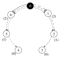
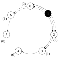
$\ldots$

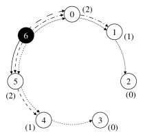
Figure 1: Routing in a ring. The numbers in parentheses represent the number of routes originating from the black node that pass through each node.

To determine the routing cost $R_{i}$, we compute the number of routes passing through a given node $i$, or node loading, as a function $L_{i,D}$ of the dimension $D$. With our assumption that the $D$-torus is equally partitioned, $L_{i,D}$ is the same for all $i$ by symmetry. We next compute $L_{i,D}$ by induction on the dimension $D$.

Base case $(D=1)$.

For $D=1$, the $D$-torus is a ring, as depicted in Figure 1 for $N=7$. Each of the diagrams in the figure corresponds to a case where the source of all requests, represented by a black node, is held fixed. The numbers in each node ($0,\ldots,6$) represent the node coordinate, the different line styles represent the different routes to all destinations, and the numbers in parentheses denote the number of routes originating from the fixed source that pass through each of the other nodes. As shown in the figure, shifting the source of all requests from 0 to $1,\ldots,6$ only results in shifting the number of routes that pass through each node. Hence, the node loading $L_{i,1}$ at each node $i$, is equal to the sum of the number of routes passing through each node when the source is held fixed. In the figure, for $N=7$, we have for any $i$, $L_{i,1}=0+1+2+2+1+0=6$. More generally, for $N$ odd, the sum of the number of routes passing through each node is equal to

$$L_{i,1} = 2\left(1+2+\ldots+\left(\frac{N-1}{2}-1\right)\right)$$ (11)

$$= \frac{(N-1)(N-3)}{4}\ ,$$

and for $N$ even, is given by

$$L_{i,1} = \left(1+2+\ldots+\left(\frac{N}{2}-1\right)\right)+\left(1+2+\ldots+\left(\frac{N}{2}-2\right)\right)$$ (12)

$$= \frac{(N-2)^{2}}{4}\ .$$

We can express Eqs. (11) and (12) in a more compact form, which holds for any $N$,

$$L_{i,1}=\left(\left\lfloor\frac{N}{2}\right\rfloor-1\right)\left(\left\lceil\frac{N}{2}\right\rceil-1\right)\ .$$ (13)

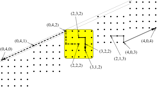
Figure 2: Routing in 3-torus. Coordinates are corrected one at a time, first along the horizontal axis, then along the vertical axis, and finally along the diagonal axis.

General case $(D>1)$.

The key observation to compute the number of routes $L_{i,D}$ passing through each node $i$ for $D>1$, is that there are several equivalent shortest paths along the Cartesian coordinates, because the coordinates of two consecutive nodes in a path cannot differ in more than one dimension. Consider for instance, for $D=2$, going from node (0,0) to node (1,1): both $\mathcal{P}_{1}=(0,0)\rightarrow(1,0)\rightarrow(1,1)$ and $\mathcal{P}_{2}=(0,0)\rightarrow(0,1)\rightarrow(1,1)$ are equivalent shortest paths. Therefore, we can always pick the path that corrects coordinates successively, starting with the first coordinate, i.e., $\mathcal{P}_{1}$ in the above example.

Consider a $D$-torus, as represented for $D=3$ in Figure 2, where each of the $N=125$ nodes is represented by a dot. The figure illustrate how requests are routed by correcting coordinates successively, with the example of three different paths, $(2,3,2)\rightarrow(3,1,2)$, $(2,2,2)\rightarrow(0,4,0)$, and $(2,1,3)\rightarrow(4,0,4)$. For any node $k$, we compute the number of routes passing through $k$. We denote the source of the route as node $i$, and the destination of the route as node $j$. We have $i\neq j\neq k$. We further denote the coordinates of $i$, $j$, and $k$ by $(i_{1},\ldots,i_{D})$, $(j_{1},\ldots,j_{D})$, and $(k_{1},\ldots,k_{D})$. We distinguish between the only three possibilities for $k$ that are allowed by the routing scheme that corrects coordinates one at a time:

1. Node $k$ has the same $D$-th coordinate as both the source $i$ and the destination $j$, i.e., $i_{D}=j_{D}=k_{D}$. In other words, the route $\mathcal{P}=i\rightarrow j$ is entirely contained within a $(D-1)$-torus. This case is illustrated in the figure for the route represented by a solid line going from $i=(2,3,2)$ to $j=(3,1,2)$ through $k=(3,2,2)$. The corresponding $(D-1)$-torus containing $i$, $j$ and $k$ is denoted by the shaded box. By definition of the node loading, the node loading resulting from all possible paths $\mathcal{P}$ contained in a $(D-1)$-torus is equal to $L_{i,D-1}$. There are $n$ different such $(D-1)$-tori in the $D$-torus under consideration, one for each possible value of $i_{D}=j_{D}=k_{D}$. So, the total load incurred on each node by all paths which remain contained within a $(D-1)$-torus is equal to $nL_{i,D-1}$.

2. Nodes $i$, $j$ and $k$ all differ in their $D$-th coordinate, i.e., $i_{D}\neq j_{D}\neq k_{D}$. Because coordinates are corrected one at a time, for any $l\in(1,\ldots,D-1)$, we must have $k_{l}=j_{l}$. This case is illustrated in the figure for the route represented by a dashed line, going from $i=(2,2,2)$ to $j=(0,4,0)$, through $k=(0,4,1)$. Since $k_{l}=j_{l}$, nodes $j$ and $k$ belong to the same ring where only the $D$-th coordinate varies. Such a ring is represented in the figure by the dotted curve. From node $k$’s perspective, routing traffic from $i$ to $j$ is equivalent to routing traffic between nodes $i^{\prime}$ and $j$, where node $i^{\prime}$ satisfies $i^{\prime}_{l}=k_{l}$ for any $l\in(1,\ldots,D-1)$, and $i^{\prime}_{D}=i_{D}$. (In the figure, the coordinates of node $i^{\prime}$ are $(0,4,2)$.) From our hypothesis $k_{D}\neq i_{D}$, we have $k_{D}\neq i^{\prime}_{D}$, which implies $k\neq i^{\prime}$. Therefore, computing the number of routes passing through node $k$ coming from $i$ is equivalent to computing the number of routes passing through node $k$ and originating from node $i^{\prime}$. Summing over all possible destination nodes $j$, the computation of all routes passing through $k$ and originating from all nodes $i^{\prime}$ in the same ring as $j$ and $k$ is identical to the computation of the node loading in the base case $D=1$. So, the load imposed on node $k$ is equal to $L_{i,1}$. Now, summing over all possible nodes $i$ is equivalent to summing over all possible rings where only the $D$-th coordinate varies. There are are $n^{D-1}$ such rings in the $D$-torus. We conclude that the total load incurred on each node $k$ by the paths going from all $i$ to all $j$ satisfying $i_{D}\neq j_{D}\neq k_{D}$ is equal to $n^{D-1}L_{i,1}$.

3. Node $k$ has the same $D$-th coordinate as node $i$, and a $D$-th coordinate different from that of the destination $j$. In other words, $i_{D}\neq j_{D}$, $i_{D}=k_{D}$. This situation is illustrated in the figure for the route going from $i=(2,1,3)$ to $j=(4,0,4)$ and passing through $k=(4,0,3)$, and represented by a thick dotted line. In this configuration, there are $(n-1)$ possible choices for the destination node $j$ such that $j_{D}\neq k_{D}$, and $j_{l}=k_{l}$ for $l\leq D-1$. There are $n^{D-1}-1$ possible choices for the source node $i$ such that $i_{D}=k_{D}$ and $i\neq j$. Hence, in this configuration, there is a total of $(n-1)(n^{D-1}-1)$ routes passing through each node $k$.

Summing the node loadings obtained in all three possible cases above, we obtain

$$L_{i,D}=nL_{i,D-1}+n^{D-1}L_{i,1}+(n-1)(n^{D-1}-1)\ .$$

Replacing $L_{i,1}$ by the expression given in Eqn. (13), using $n=N^{1/D}$, and removing the recursion in the above relationship, we obtain, for any node $i$,

$$L_{i,D}=N^{\frac{D-1}{D}}\left(D\left(N^{\frac{1}{D}}-1+\left(\left\lfloor\frac{N^{\frac{1}{D}}}{2}\right\rfloor-1\right)\left(\left\lceil\frac{N^{\frac{1}{D}}}{2}\right\rceil-1\right)\right)-N^{\frac{1}{D}}\right)+1\ .$$

For all $i$, $R_{i}$ immediately follows from $L_{i,D}$ with

$$R_{i}=r\frac{L_{i,D}}{N^{2}}\ .$$

Plaxton trees

We next consider the variant of Plaxton trees [17] used in Pastry [19] or Tapestry [22]. Nodes are represented by a string $(i_{1},\ldots,i_{D})$ of $D$ digits in base $\Delta$. Each node is connected to $D(\Delta-1)$ distinct neighbors of the form $(i_{1},\ldots,i_{l-1},x,y_{l+1},\ldots,y_{D})$, for $l=1\ldots D$, and $x\neq i_{l}\in\{0,\ldots,\Delta-1\}$. The resulting maintenance cost is $M_{i}=mD(\Delta-1)$.

Among the different possibilities for the remaining coordinates $y_{l+1},\ldots,y_{D}$, the protocols generally select a node that is nearby according to a spatial proximity metric. We here assume that the spatial distribution of the nodes is uniform, and that the identifier space is fully populated (i.e., $N=\Delta^{D}$), which enables us to pick $y_{l+1}=i_{l+1},\ldots,y_{D}=i_{D}$. Thus, two nodes $i$ and $j$ at a distance of $k$ hops differ in $k$ digits. There are $D\choose k$ ways of choosing which digits are different, and each such digit can take any of $(\Delta-1)$ values. So, for a given node $i$, there are ${D\choose k}(\Delta-1)^{k}$ nodes that are at distance $k$ from $i$. Multiplying by the total number of nodes $N=\Delta^{D}$, and dividing by the total number of paths $N^{2}$, we infer that, for all $i$, $j$, and $k$, we have

$$\mbox{Pr}[t_{i,j}=k]=\frac{{D\choose k}(\Delta-1)^{k}}{N}\ .$$ (14)

Now, for any $i$ and $j$ such that $t_{i,j}=l$, because routes are unique, there are exactly $(l-1)$ different nodes on the path between $i$ and $j$. So, the probability that a node $k$ picked at random is on the path from $i$ to $j$ is

$$\mbox{Pr}[\chi_{i,j}(k)=1|t_{i,j}=l]=\frac{l-1}{N}\ .$$ (15)

The total probability theorem tells us that

$$\mbox{Pr}[\chi_{i,j}(k)=1]=\sum_{l=1}^{D}\mbox{Pr}[\chi_{i,j}(k)=1|t_{i,j}=l]\cdot\mbox{Pr}[t_{i,j}=l]\ .$$

Substituting with the expressions obtained for $\mbox{Pr}[t_{i,j}=l]$ and $\mbox{Pr}[\chi_{i,j}(k)=1|t_{i,j}=l]$ in Eqs. (14) and (15) gives:

$$\mbox{Pr}[\chi_{i,j}(k)=1]=\frac{1}{N^{2}}\sum_{l=1}^{D}(l-1){D\choose l}(\Delta-1)^{l}\ ,$$ (16)

which can be simplified as follows. We write:

$$\sum_{l=1}^{D}{D\choose l}(l-1)(\Delta-1)^{l}=(\Delta-1)^{2}\sum_{l=1}^{D}(l-1){D\choose l}(\Delta-1)^{l-2}\ ,$$

and rewrite the right-hand term as a function of the derivative of a series,

$$\sum_{l=1}^{D}{D\choose l}(l-1)(\Delta-1)^{l}=(\Delta-1)^{2}\frac{\partial}{\partial\Delta}\left(\sum_{l=1}^{D}{D\choose l}(\Delta-1)^{l-1}\right)\ ,$$

or, equivalently,

$$\sum_{l=1}^{D}{D\choose l}(l-1)(\Delta-1)^{l}=(\Delta-1)^{2}\frac{\partial}{\partial\Delta}\left(\frac{1}{\Delta-1}\sum_{l=1}^{D}{D\choose l}1^{D-l}(\Delta-1)^{l}\right)\ .$$

The binomial theorem allows us to simplify the above to:

$$\sum_{l=1}^{D}{D\choose l}(l-1)(\Delta-1)^{l}=(\Delta-1)^{2}\frac{\partial}{\partial\Delta}\left(\frac{1}{\Delta-1}(1+\Delta-1)^{D}-1\right)\ ,$$

which, making the partial derivative explicit, becomes,

$$\sum_{l=1}^{D}{D\choose l}(l-1)(\Delta-1)^{l}=(\Delta-1)^{2}\left(\frac{D\Delta^{D-1}(\Delta-1)-\Delta^{D}+1}{(\Delta-1)^{2}}\right)\ ,$$

and reduces to

$$\sum_{l=1}^{D}{D\choose l}(l-1)(\Delta-1)^{l}=\Delta^{D-1}(D(\Delta-1)-\Delta)+1\ .$$

Substituting in Eqn. (16) gives:

$$\mbox{Pr}[\chi_{i,j}(k)=1]=\frac{\Delta^{D-1}(D(\Delta-1)-\Delta)+1}{N^{2}}\ ,$$

which we multiply by $r$ to obtain

$$R_{i}=r\frac{\Delta^{D-1}(D(\Delta-1)-\Delta)+1}{N^{2}}\ .$$ (17)

To compute the access cost $A_{i}$, we use the relationship $A_{i}=aE[t_{i,j}]$. We have

$$E[t_{i,j}]=\sum_{k=1}^{D}k\mbox{Pr}[t_{i,j}=k]\ ,$$

which, using the expression for $\mbox{Pr}[t_{i,j}=k]$ given in Eqn. (14), implies

$$E[t_{i,j}]=\sum_{k=0}^{D}k\frac{{D\choose k}(\Delta-1)^{k}}{N}\ ,$$

and can be expressed in terms of the derivative of a classical series:

$$E[t_{i,j}]=\frac{\Delta-1}{N}\frac{\partial}{\partial\Delta}\left(\sum_{k=0}^{D}{D\choose k}(\Delta-1)^{k}\right)\ .$$

Using the binomial theorem, the series on the right-hand side collapses to $\Delta^{D}$, which yields

$$E[t_{i,j}]=\frac{\Delta-1}{N}\frac{\partial(\Delta^{D})}{\partial\Delta}\ .$$

We compute the partial derivative, and obtain

$$E[t_{i,j}]=\frac{D\Delta^{D-1}(\Delta-1)}{N}\ .$$

Multiplying by $a$ to obtain $A_{i}$, we eventually get, for all $i$,

$$A_{i}=a\frac{D\Delta^{D-1}(\Delta-1)}{N}\ ,$$

which can be simplified, using $N=\Delta^{D}$:

$$A_{i}=aD\frac{\Delta-1}{\Delta}\ .$$ (18)

Chord rings

In a Chord ring [21], nodes are represented using a binary string (i.e., $\Delta=2$). When the ring is fully populated, each node $i$ is connected to a set of $D$ neighbors, with identifiers $((i+2^{m})\mod 2^{D})$ for $m=0\ldots D-1$. An analysis identical to the above yields $R_{i}$ and $A_{i}$ as in Eqs. (17) and (18) for $\Delta=2$. Note that Eqn. (18) with $\Delta=2$ is confirmed by experimental measurements [21].

3.2 Numerical results

$(\Delta,D)$	$A_{\min}$	$A_{\max}$	$\frac{A_{\max}}{A_{\min}}$	$R^{\prime}_{\min}$	$R_{\max}$	$\frac{R_{\max}}{R^{\prime}_{\min}}$
(2, 9)	7.18	8.00	1.11	3.89	17.53	4.51
(3, 6)	5.26	5.50	1.04	2.05	9.05	4.41
(4, 4)	3.56	3.67	1.03	5.11	13.87	2.71
(5, 4)	3.69	3.75	1.02	1.98	5.50	2.78
(6, 3)	2.76	2.80	1.01	5.38	9.99	1.86

Table 1: Asymmetry in costs in a de Bruijn graph $(a=1,r=1000)$

We illustrate our analysis with a few numerical results. In Table 1, we consider five de Bruijn graphs with different values for $\Delta$ and $D$, and $X$ and $Y$ i.i.d. uniform random variables. Table 1 shows that while the access costs of all nodes are comparable, the ratio between $R_{\max}$ and the second best case routing cost, $R^{\prime}_{\min}$, is in general significant. Thus, if $r\gg a$, there can be an incentive for the nodes with $R_{i}=R_{\max}$ to defect. For instance, these nodes may leave the network and immediately come back, hoping to be assigned a different identifier $i^{\prime}\neq i$ and incurring a lower cost. Additional mechanisms, such as enforcing a cost of entry to the network, may be required to prevent such defections.

(a) Access cost $(a=1)$

(b) Routing cost $(r=1000)$

Figure 3: Costs in a de Bruijn network with $\Delta=5$, $D=4$ and $N=625$

We graph the access and routing costs for the case $\Delta=5$, $D=4$ and $N=625$ in Figure 3. We plot the access cost of each node in function of the node identifier in Figure 3(a), and the routing cost of each node in function of the node identifier in Figure 3(b). Figure 3 further illustrates the asymmetry in costs evidenced in Table 1, by exhibiting that different nodes have generally different access and routing costs. Therefore, in a de Bruijn graph, there is potentially a large number of nodes that can defect, which, in turn, may result in network instability, if defection is characterized by leaving and immediately rejoining the network.

Next, we provide an illustration by simulation of the costs in the different geometries. We choose $\Delta=2$, for which the results for Plaxton trees and Chord rings are identical. We choose $D=\{2,6\}$ for the $D$-dimensional tori, and $D=\log_{\Delta}N$ for the other geometries. We point out that selecting a value for $D$ and $\Delta$ common to all geometries may inadvertently bias one geometry against another. We emphasize that we only illustrate a specific example here, without making any general comparison between different DHT geometries.

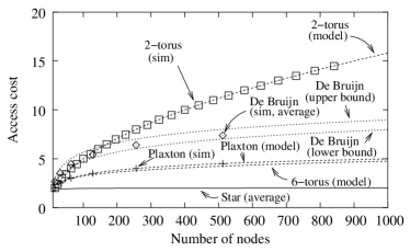
(a) Access cost $(a=1)$

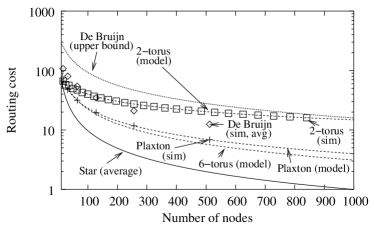
(b) Routing cost $(r=1000)$

Figure 4: Access and routing costs. Curves marked “sim” present simulation results.

We vary the number of nodes between $N=10$ and $N=1000$, and, for each value of $N$ run ten differently seeded simulations, consisting of 100,000 requests each, with $X$ and $Y$ i.i.d. uniform random variables. We plot the access and routing costs averaged over all nodes and all requests in Figure 4. The graphs show that our analysis is validated by simulation, and that the star provides a lower average cost than all the other geometries. In other words, a centralized architecture appears more desirable to the community as a whole than a distributed solution. However, we stress that we do not consider robustness against attack, fault-tolerance, or potential performance bottlenecks, all being factors that pose practical challenges in a centralized approach, nor do we offer a mechanism creating an incentive to be in the center of the star. While the cost model proposed here can be used to quantify the cost incurred by adding links for a higher resiliency to failures, we defer that study to future work.

4 Discussion

We proposed a model, based on experienced load and node connectivity, for the cost incurred by each peer to participate in a peer-to-peer network. We argue such a cost model is a useful complement to topological performance metrics [7, 12], in that it allows to predict disincentives to collaborate (peers refusing to serve requests to reduce their cost), discover possible network instabilities (peers leaving and re-joining in hopes of lowering their cost), identify hot spots (peers with high routing load), and characterize the efficiency of a network as a whole.

We believe however that this paper raises more questions than it provides answers. First, we only analyzed a handful of DHT routing geometries, and even omitted interesting geometries such as the butterfly [13], or geometries based on the XOR metric [14]. Applying the proposed cost model to deployed peer-to-peer systems such as Gnutella or FastTrack could yield some insight regarding user behavior. Furthermore, for the mathematical analysis, we used strong assumptions such as identical popularity of all items and uniform spatial distribution of all participants. Relaxing these assumptions is necessary to evaluate the performance of a geometry in a realistic setting. Also, obtaining a meaningful set of values for the parameters $(s,a,r,m)$ for a given class of applications (e.g., file sharing between PCs, ad-hoc routing between energy-constrained sensor motes) remains an open problem. Finally, identifying the minimal amount of knowledge each node should possess to devise a rational strategy, or studying network formation with the proposed cost model are other promising avenues for further research.

References

- [1] The annotated Gnutella protocol specification v0.4, June 2001. http://rfc-gnutella.sourceforge.net/developer/stable/index.html.
- [2] S. Banerjee, B. Bhattacharjee, and C. Kommareddy. Scalable application layer multicast. In Proceedings of ACM SIGCOMM’02, pages 205–217, Pittsburgh, PA, August 2002.
- [3] Y.-H. Chu, S. Rao, and H. Zhang. A case for endsystem multicast. In Proceedings of ACM SIGMETRICS’00, pages 1–12, Santa Clara, CA, June 2000.
- [4] B.-G. Chun, R. Fonseca, I. Stoica, and J. Kubiatowicz. Characterizing selfishly constructed overlay networks. In Proceedings of IEEE INFOCOM’04, Hong Kong, March 2004. To appear.
- [5] C. Perkins (ed). Ad hoc networking. Addison-Wesley, Boston, MA, 2000.
- [6] A. Fabrikant, A. Luthra, E. Maneva, C. Papadimitriou, and S. Shenker. On a network creation game. In Proceedings of ACM PODC’03, pages 347–351, Boston, MA, July 2003.
- [7] K. Gummadi, R. Gummadi, S. Gribble, S. Ratnasamy, S. Shenker, and I. Stoica. The impact of DHT routing geometry on resilience and proximity. In Proceedings of ACM SIGCOMM’03, pages 381–394, Karlsruhe, Germany, August 2003.
- [8] M. Hefeeda, A. Habib, B. Botev, D. Xu, and B. Bhargava. Promise: Peer-to-peer media streaming using CollectCast. In Proceedings of ACM Multimedia’03, pages 45–54, Berkeley, CA, November 2003.
- [9] M. Jackson and A. Wolinsky. A strategic model for social and economic networks. Journal of Economic Theory, 71(1):44–74, October 1996.
- [10] M. F. Kaashoek and D. Karger. Koorde: A simple degree-optimal distributed hash table. In Proceedings of the 2nd International Workshop on Peer-to-Peer Systems (IPTPS’03), pages 323–336, Berkeley, CA, February 2003.
- [11] J. Liebeherr, M. Nahas, and W. Si. Application-layer multicast with Delaunay triangulations. IEEE Journal of Selected Areas in Communications, 20(8):1472–1488, October 2002.
- [12] D. Loguinov, A. Kumar, V. Rai, and S. Ganesh. Graph-theoretic analysis of structured peer-to-peer systems: routing distances and fault resilience. In Proceedings of ACM SIGCOMM’03, pages 395–406, Karlsruhe, Germany, August 2003.
- [13] D. Malkhi, M. Naor, and D. Ratajczak. Viceroy: a scalable and dynamic emulation of the butterfly. In Proceedings of ACM PODC’02, pages 183–192, Monterey, CA, July 2002.
- [14] P. Maymounkov and D. Mazières. Kademlia: A peer-to-peer information system based on the XOR metric. In Proceedings of the 1st International Workshop on Peer-to-Peer Systems (IPTPS’02), pages 53–65, Cambridge, MA, February 2002.
- [15] M. Naor and U. Wieder. Novel architectures for P2P applications: the continuous-discrete approach. In Proceedings of ACM SPAA’03, pages 50–59, San Diego, CA, June 2003.
- [16] C. Ng, D. Parkes, and M. Seltzer. Strategyproof computing: Systems infrastructures for self-interested parties. In Proceedings of the 1st Workshop on the Economics of Peer-to-Peer Systems, Berkeley, CA, June 2003.
- [17] C. G. Plaxton, R. Rajamaran, and A. Richa. Accessing nearby copies of replicated objects in a distributed environment. Theory of Computing Systems, 32(3):241–280, June 1999.
- [18] S. Ratnasamy, P. Francis, M. Handley, R. Karp, and S. Shenker. A scalable content-addressable network. In Proceedings of ACM SIGCOMM’01, pages 161–172, San Diego, CA, August 2001.
- [19] A. Rowston and P. Druschel. Pastry: Scalable, decentralized object location and routing for large scale peer-to-peer systems. In Proceedings of the 18th IFIP/ACM International Conference on Distributed Systems Platform (Middleware’01), pages 329–350, Heidelberg, Germany, November 2001.
- [20] K. Sivarajan and R. Ramaswami. Lightwave networks based on de Bruijn graphs. IEEE/ACM Transactions on Networking, 2(1):70–79, February 1994.
- [21] I. Stoica, R. Morris, D. Liben-Nowell, D. Karger, M. F. Kaashoek, and H. Balakrishnan. Chord: A scalable peer-to-peer lookup protocol for Internet applications. IEEE/ACM Transactions on Networking, 11(1):17–32, February 2003.
- [22] B. Zhao, L. Huang, J. Stribling, S. Rhea, A. Joseph, and J. Kubiatowicz. Tapestry: A resilient global-scale overlay for service deployment. IEEE Journal on Selected Areas in Communications, 2004. To appear.