On Addressing Efficiency Concerns in Privacy-Preserving Mining

Abstract

Data mining services require accurate input data for their results to be meaningful, but privacy concerns may influence users to provide spurious information. To encourage users to provide correct inputs, we recently proposed a data distortion scheme for association rule mining that simultaneously provides both privacy to the user and accuracy in the mining results. However, mining the distorted database can be orders of magnitude more time-consuming as compared to mining the original database. In this paper, we address this issue and demonstrate that by (a) generalizing the distortion process to perform symbol-specific distortion, (b) appropriately chooosing the distortion parameters, and (c) applying a variety of optimizations in the reconstruction process, runtime efficiencies that are well within an order of magnitude of undistorted mining can be achieved.

1 Introduction

The knowledge models produced through data mining techniques are only as good as the accuracy of their input data. One source of data inaccuracy is when users deliberately provide wrong information. This is especially common with regard to customers who are asked to provide personal information on Web forms to e-commerce service providers. The compulsion for doing so may be the (perhaps well-founded) worry that the requested information may be misused by the service provider to harass the customer. As a case in point, consider a pharmaceutical company that asks clients to disclose the diseases they have suffered from in order to investigate the correlations in their occurrences – for example, “Adult females with malarial infections are also prone to contract tuberculosis”. While the company may be acquiring the data solely for genuine data mining purposes that would eventually reflect itself in better service to the client, at the same time the client might worry that if her medical records are either inadvertently or deliberately disclosed, it may adversely affect her employment opportunities.

Recently, in [11], we investigated (for the first time) whether customers can be encouraged to provide correct information by ensuring that the mining process cannot, with any reasonable degree of certainty, violate their privacy, but at the same time produce sufficiently accurate mining results. The difficulty in achieving these goals is that privacy and accuracy are typically contradictory in nature, with the consequence that improving one usually incurs a cost in the other [2].

Our study was carried out in the context of extracting association rules from large historical databases, a popular mining process [3] that identifies interesting correlations between database attributes, such as the one described in the pharmaceutical example. For this framework, we presented a scheme called MASK, (Mining Associations with Secrecy Konstraints), based on a simple probabilistic distortion of user data, employing random numbers generated from a pre-defined distribution function. It is this distorted information that is eventually supplied to the data miner, along with a description of the distortion procedure. A special feature of MASK is that the distortion process can be implemented at the data source itself, that is, at the user machine. This increases the confidence of the user in providing accurate information since she does not have to trust a third-party to distort the data before it is acquired by the service provider.

Experimental evaluation of MASK on a variety of synthetic and real datasets showed that, by appropriate setting of the distortion parameters, it was possible to simultaneously achieve a high degree of privacy and retain a high degree of accuracy in the mining results. While these results were very encouraging, a problem left unaddressed was characterizing the runtime efficiency of mining the distorted data as compared to directly mining the original data. That is, the question “Is privacy-preserving mining of association rules more expensive than direct mining?” was not considered in detail. Our subsequent analysis has shown that this issue is indeed a major concern: Specifically, we have found that on typical market-basket databases, privacy-preserving mining can take as much as two to three orders of magnitude more time as compared to direct mining. Such enormous overheads raise serious questions about the viability of supporting privacy concerns in data mining environments.

In this paper, we address the runtime efficiency issue in privacy-preserving association rule mining, which to the best of our knowledge has never been previously considered in the literature. Within this framework, our contributions are the following:

• We show that there are inherent reasons as to why mining the distorted database is a significantly harder exercise as compared to directly mining the original database.

• We demonstrate that it is possible to bring the efficiency to well within an order of magnitude with respect to direct mining, while retaining satisfactory privacy and accuracy levels. This improvement is achieved through changes in both the distortion process and the mining process of MASK, resulting in a new algorithm that we refer to as EMASK. In EMASK, the distortion process is generalized to perform symbol-specific distortion – that is, different distortion parameters are used for 1’s and 0’s in a transaction.(1 indicates the presence of an item and 0 indicates the absence of an item in a transaction). Estimation procedures are designed to carefully chose the parameters of distortion beforehand and a variety of optimizations are applied in the mining process to achieve the desired goals. Our new design is validated against a variety of synthetic and real datasets.

• In MASK, privacy is measured with respect to the ability to directly reconstruct entries in the distorted matrix. We refer to this hereafter as “basic privacy”. In EMASK, we consider basic privacy as well as “reinterrogated privacy” – this latter notion captures the situation wherein the miner is permitted to utilize the mining output (i.e. the association rules) to reinterrogate the distorted matrix, potentially resulting in reduced privacy.

1.1 Organization

The remainder of this paper is organized as follows: In Section 2, we describe the privacy framework employed in our study, while Section 3 provides background information about the original MASK algorithm. Then, in Section 4, we present the details of our new EMASK privacy-preserving scheme. The performance model and the experimental results are highlighted in Sections 5 and 6, respectively. Related work on privacy-preserving mining is reviewed in Section 7. Finally, in Section 8, we summarize the conclusions of our study.

2 Problem Framework

2.1 Database Model

We assume that each customer contributes a tuple to the database with the tuple being a fixed-length sequence of 1’s and 0’s. A typical example of such a database is the so-called “market-basket” database [3] wherein the columns represent the items sold by a supermarket, and each row describes, through a sequence of 1’s and 0’s, the purchases made by a particular customer (1 indicates a purchase and 0 indicates no purchase). We also assume that the overall number of 1’s in the database is significantly smaller than the number of 0’s – this is especially true for market-baskets since each customer typically buys only a small fraction of all the items available in the store. In short, the database is modeled as a large disk-resident two-dimensional sparse boolean matrix.

Note that the boolean representation is only logical and that the database tuples may actually be physically stored as “item-lists”, that is, as an ordered list of the identifiers of the items purchased in the transaction. The list representation may appear preferable for the sparse databases that we are considering, since it reduces the space requirement as compared to storing entire bit-vectors. However, because we are distorting user information, it may be the case that the distorted matrix will not be as sparse as the true database. Therefore, in this paper, we assume that the distorted database is stored as a large collection of bit-vectors.

2.2 Mining Objectives

The goal of the miner is to compute association rules on the above database. Denoting the set of transactions in the database by ${\cal T}$ and the set of items in the database by $\cal I$, an association rule is a (statistical) implication of the form $\cal X\Longrightarrow Y$, where ${\cal X,\cal Y\subset\cal I}$ and ${\cal X}\cap Y=\phi$. A rule $\cal X\Longrightarrow Y$ is said to have a support (or frequency) factor s iff at least ${s}\%$ of the transactions in ${\cal T}$ satisfy $\cal X\cup Y$. A rule $\cal X\Longrightarrow Y$ is satisfied in the set of transactions ${\cal T}$ with a confidence factor c iff at least $c\%$ of the transactions in ${\cal T}$ that satisfy $\cal X$ also satisfy $\cal Y$. Both support and confidence are fractions in the interval [0,1]. The support is a measure of statistical significance, whereas confidence is a measure of the strength of the rule.

A rule is said to be “interesting” if its support and confidence are greater than user-defined thresholds ${sup}_{min}$ and ${con}_{min}$, respectively, and the objective of the mining process is to find all such interesting rules. It has been shown in [3] that achieving this goal is effectively equivalent to generating all subsets $\cal X$ of $\cal I$ that have support greater than ${sup}_{min}$ – these subsets are called frequent itemsets. Therefore, the mining objective is, in essence, to efficiently discover all frequent itemsets that are present in the database.

2.3 Privacy Metric

As mentioned earlier, the mechanism adopted in this paper for achieving privacy is to distort the user data before it is subject to the mining process. Accordingly, we measure privacy with regard to the probability with which distorted entries can be reconstructed. In short, our privacy metric is: “With what probability can a random 1 or 0 in the true matrix be reconstructed”? For the sake of presentation simplicity, we will assume in the sequel that the user is only interested in privacy for 1’s (this appears reasonable to expect in a market-basket environment, since the 1’s denote specific actions, whereas the 0’s are default options). The generalization to providing privacy for both 1’s and 0’s is straightforward – the details are given in [1].

Privacy can be computed at two levels: Basic Privacy (BP) and Re-interrogated Privacy (RP). In basic privacy, we assume that the miner does not have access to the distorted data matrix after the completion of the mining process. Whereas, in re-interrogated privacy, the miner can use the mining output (i.e. the association rules) to subsequently re-interrogate the distorted database, possibly resulting in reduced privacy.

3 Background on MASK

We present here background information on the MASK algorithm, which we recently proposed in [11] for providing acceptable levels of both privacy and accuracy.

Given a customer tuple with 1’s and 0’s, the MASK algorithm has a simple distortion process: Each item value (i.e. 1 or 0) is either kept the same with probability $p$ or is flipped with probability $1-p$. All the customer tuples are distorted in this fashion and make up the database supplied to the miner – in effect, the miner receives a probabilistic function of the true customer database. For this distortion process, the Basic Privacy for 1’s was computed to be

$$\textstyle{{\cal R}_{1}(p)=\frac{s_{0}\times p^{2}}{s_{0}\times p+(1-s_{0})\times(1-p)}+\frac{s_{0}\times(1-p)^{2}}{s_{0}\times(1-p)+(1-s_{0})\times p}}$$ (1)

where $s_{0}$ is the average support of individual items in the database and $p$ is the distortion parameter mentioned above.

Since the privacy graph as a function of $p$ has a large range where it is almost constant, it means that we have considerable flexibility in choosing the $p$ value – in particular, we can choose it in a manner that will minimize the error in the subsequent mining process. Specifically, the experiments in [11] showed that choosing $p=0.9$ (or, equivalently, $p=0.1$, since the graph is symmetric about $p=0.5$) was most conducive to accuracy.

The concept of Re-interrogated Privacy was not considered in [11]; we include it in this paper and compute both Basic Privacy and Re-interrogated Privacy for EMASK (see Section 4.1.1 for details).

4 The EMASK Algorithm

Our motivation for the EMASK algorithm stems from the fact that while MASK is successful in obtaining the dual objectives of privacy and accuracy, its runtime efficiency proves to be rather poor. To motivate the cause for this inefficiency, let us look at the performance numbers of a sample database. Figure 1 shows the running time (on log scale) of MASK as compared to Apriori for a synthetic database generated with IBM Synthetic Data generator (T10.I4.D1M.N1K as per naming convention of [4]). The figure shows that there are huge differences in running times of the two algorithms – specifically, mining the distorted database can take as much as two to three orders of magnitude more time than mining the original database. Obviously, such enormous overheads make it difficult for MASK to be viable in practice.

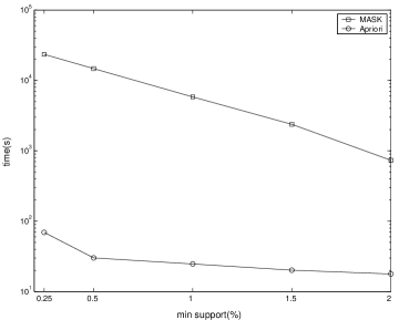
Figure 1: Comparison of run time of Apriori and MASK (log scale)

The reason for the huge overheads are the following:

Increased database density:

This overhead is inherent to the methods employing random distortion method to achieve privacy. The random perturbation methods flip 0’s to 1’s to hide the original 1’s. Due to the generation of false 1’s, the density of the database matrix is increased considerably. For example, given a supermarket database with an average transaction length of 10 over a 1000 item inventory, a flipping probability as low as 0.1 increases the average transaction length by an order of magnitude, i.e. from 10 to 108. The reason that flipping of true 1’s to false 0’s cannot compensate for this increase is that the datasets we are considering here are sparse databases, with the number of 0’s orders of magnitude larger than the number of 1’s. Hence the effect of flipping 0’s highly dominates the effect of flipping 1’s.

As a result of increased transaction lengths, counting the itemsets in the distorted database requires much more processing as compared to the original database, substantially increasing the mining time. In [9], a technique for compressing large transactions is proposed – however, its utility is primarily in reducing storage and communication cost, and not in reducing the mining runtime since the compressed transactions have to be decompressed during the mining process.

Counting Overhead:

On distortion, a $k$-itemset may produce any of $2^{k}$ combinations. For example, a ’11’ may distort to ’00’,’01’,’10’ or ’11’. In order to accurately reconstruct the support of the $k$-itemset, we need to, in principle, keep track of the counts of all $2^{k}$ combinations. To reduce these costs, MASK took the approach of maintaining equal flipping probabilities for both 1’s and 0’s – with this assumption, the number of counters required is only $k$ [11]. Further, only $k-1$ of the counts need to be explicitly maintained since the sum of the counts is equal to the database cardinality, $dbsize$ – the counter chosen to be implicitly counted was the one with the expected largest count.

While the above counting optimizations did appreciably reduce runtime costs, yet the overhead in absolute terms remains very significant – as mentioned earlier, it could be as much as two to three orders of magnitude compared to the time taken for direct mining.

In the remainder of this section, we describe how EMASK is engineered to address the above efficiency concerns.

4.1 The Distortion Process

The new feature of EMASK’s distortion process is that it applies symbol-specific distortion – that is, 1’s are flipped with probability $(1-p)$, while 0’s are flipped with probability $(1-q)$. Note that in this framework the original MASK can be viewed as a special case of EMASK wherein $p=q$.

The idea here is that MASK generates false items to hide the true items that are retained after distortion, resulting in an increase in database density. But, if a fewer number of true items are retained, a fewer number of false items need to be generated, and we can minimize this density increase. Thus the goal of reduced density could be achieved by reducing the value of $p$ and increasing the value of $q$ (specifically increasing it to beyond 0.9). However, note that a decrease in $p$ value increases the distortion significantly which can reduce accuracy of reconstruction. Also, $q$ or the non-flipping probability of 0s cannot be increased to very high values as it can decrease the privacy significantly. Thus the choices of $p$ and $q$ have to be made carefully to obtain a combination of $p$ and $q$ values, such that $q$ is high enough to result in decreased transaction lengths but privacy and accuracy are still achievable.

We defer the discussion on how to select appropriate values of $p$ and $q$ to Section 4.4.

4.1.1 Privacy Estimation for EMASK

As mentioned earlier, privacy can be computed at two levels: Basic Privacy (BP) and Reinterrogated Privacy (RP). We now quantify the privacy provided by EMASK with regard to both these metrics.

4.1.2 Basic Privacy

The basic privacy measures the probability that given a random customer $C$ who bought an item $i$, her original entry for $i$, i.e. ’1’, can be accurately reconstructed from the distorted entry, prior to the mining process. We can calculate this privacy in the following manner, similar to the procedure outlined for MASK in [11]: Let $s_{i}$ be the support of the $i^{th}$ item, $X_{i}$ be the original entry corresponding to item $i$, in a tuple and $Y_{i}$ be its distorted entry. The reconstruction probability of a $1$ is given by

$$R_{1}(p,q,s_{i})=\Pr(Y_{i}=1|X_{i}=1)\Pr(X_{i}=1|Y_{i}=1)+\Pr(Y_{i}=0|X_{i}=1)\Pr(X_{i}=1|Y_{i}=0)$$

$$=\frac{{\Pr(Y_{i}=1|X_{i}=1)}^{2}\Pr(X_{i}=1)}{\Pr(Y_{i}=1)}+\frac{{\Pr(Y_{i}=0|X_{i}=1)}^{2}\Pr(X_{i}=1)}{\Pr(Y_{i}=0)}$$

$$=\frac{p^{2}s_{i}}{\Pr(Y_{i}=1)}+\frac{(1-p)^{2}s_{i}}{\Pr(Y_{i}=0)}$$

But,

$$\Pr(Y_{i}=1)=\Pr(Y_{i}=1|X_{i}=0)\Pr(X_{i}=0)+\Pr(Y_{i}=1|X_{i}=1)\Pr(X_{i}=1)$$

$$=s_{i}p+(1-s_{i})(1-q)$$

And,

$$\Pr(Y_{i}=0)=1-\Pr(Y_{i}=1)=s_{i}(1-p)+(1-s_{i})q$$

Therefore,

$$R_{1}(p,q,s_{i})=\frac{p^{2}s_{i}}{s_{i}p+(1-s_{i})(1-q)}+\frac{(1-p)^{2}s_{i}}{s_{i}(1-p)+(1-s_{i})q}$$

The overall reconstruction probability of 1’s is now given by

$$R_{1}(p,q)=\frac{\sum_{i}s_{i}R_{1}(p,q,s_{i})}{\sum_{i}s_{i}}$$

and the Basic privacy offered to 1’s is simply $100(1-R_{1}(p,q))$.

The above expression is minimized when all the items in the database have the same support, and increases with the variance in the supports across items. As discussed later in Section 6, with the appropriate choices of $p$ and $q$, this increase is marginal for the market-basket type of datasets that we consider here. Therefore, as a first-level approximation, we replace the item-specific supports in the above equation by $s_{0}$, the average support of an item in the database. With this, the reconstruction probability simplifies to

$$\textstyle R_{1}(p,q)=\frac{p^{2}s_{0}}{s_{0}p+(1-s_{0})(1-q)}+\frac{(1-p)^{2}s_{0}}{s_{0}(1-p)+(1-s_{0})q}$$ (2)

In Figure 2 we plot $100(1-R_{1}(p,q))$ i.e. privacy for different values of $p$ and $q$ at $s_{0}$=0.01 – the shadings indicate the privacy ranges. Note that the color of each square represents the privacy value of the lower left corner of the square. We observe here that there is a band of values for $p$ and $q$ in which the privacy is greater than the 80% mark. Specifically, for $q$ between $0.1$ and $0.9$, high privacy values are attainable for all $p$ values, and the whole of this region appears black. Beyond $q=0.9$, privacy above 80% is attainable but only for low $p$ values. Similarly for $q$ below 0.1, high privacy can be obtained only at high $p$ values.

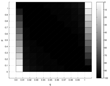
Figure 2: Basic Privacy of EMASK

4.1.3 Reinterrogation privacy

Reinterrogation privacy takes into account the reduction in privacy due to the knowledge of the output of the mining process – namely, the association rules, or equivalently, the support of frequent itemsets [4]. Privacy breach due to reinterrogation stems from the fact that an individual entry in the distorted database may not reveal enough information to reconstruct it, but on seeing a long frequent itemset in the distorted database and knowing the distorted and original supports of the itemset one may be able to predict the presence of an item of the itemset with more certainty. As an example situation, suppose the reconstructed support of a 3-itemset present in a transaction distorted with $p=0.9,q=0.9$, is 0.01. Then the probabiity of this 3-itemset coming from a ’000’ in the original transaction is as low as $0.1*0.1*0.1*0.99=0.00099$. Thus, with the knowledge of support of higher length itemsets the miner can predict the presence of an item of the itemset in the original transaction with higher probability.

Our method of estimating reinterrogation privacy breach is based on that described in [8] for computing privacy breaches. We make the extremely conservative assumption here that the data miner is able to accurately estimate the exact supports of the original database during the mining process. The method of calculating reinterrogation privacy is as follows:

• First, for each item that is part of a frequent itemset, we compare the support of the frequent itemset in the distorted data with the support of the singleton item in the original data. For example, let an itemset {a,b,c} occur a hundred times in the randomized data and let the support of the item $b$ in the corresponding hundred transactions of the original database be twenty. We then say that the itemset {a,b,c} caused a 20% privacy breach for item $b$ due to reinterrogation, since for these hundred distorted transactions, we estimate with 20% confidence that the item $b$ was present in the original transaction.

• Then, we estimate the privacy of each ’1’ appearing in a frequent item column in the original database. There are two cases: 1’s that have remained 1’s in the distorted database, and 1’s that have been flipped to 0’s. For the former, the privacy is estimated with regard to the worst of the privacy breaches (computed as discussed above) among all the frequent itemsets of which it is a part and which appear in the distorted version of this transaction. For example, for an item $b$ in the original transaction {a,b,c,d,e}, the privacy breach of $b$ is the worst of the privacy breaches due to all frequent itemsets which are subsets of {a,b,c,d,e} and contain $b$.

  In the latter (flip) case, the privacy is set equal to the average Basic Privacy value – this is because for the $q$ values that we consider in this paper, which are close to 1.0 as discussed later, most of the large number of $0$’s in the original sparse matrix remain $0$, so a $1$ flipping to a $0$ is resistant to privacy breaches due to reinterrogation.

• Next, for the 1’s present in in-frequent columns, the privacy is estimated to be the Basic Privacy since these privacies are not affected by the discovery of frequent itemsets.

• Finally, the above privacy estimates are averaged over all 1’s in the original database to obtain the overall average reinterrogation privacy.

4.2 The EMASK Mining Process

Having established the privacy obtained by EMASK’s distortion process, we now move on to presenting EMASK’s technique for estimating the true supports of itemsets from the distorted database. In the following discussion, we first show how to estimate the supports of 1-itemsets (i.e. singletons) and then present the general $n$-itemset support estimation procedure. In this derivation, it is important to keep in mind that the miner is provided with both the distorted matrix as well as the distortion procedure, that is, he knows the values of $p$ and $q$ that were used in distorting the true matrix.

4.2.1 Estimating Singleton supports

We denote the original true matrix by $T$ and the distorted matrix, obtained with distortion parameters $p$ and $q$, as $D$. Now consider a random individual item $\bf{i}$. Let $c^{T}_{1}$ and $c^{T}_{0}$ represent the number of 1’s and 0’s, respectively, in the $\bf{i}$ column of ${T}$, while $c^{D}_{1}$ and $c^{D}_{0}$ represent the number of 1’s and 0’s, respectively, in the $\bf{i}$ column of ${D}$. With this notation, we estimate the support of $\bf{i}$ in $T$ using the following equation:

$$\bf{C^{T}=M^{-1}C^{D}}$$ (3)

where

$$M=\left[\begin{array}[]{cc}p&1-q\\ 1-p&q\end{array}\right]\;C^{D}=\left[\begin{array}[]{c}c^{D}_{1}\\ c^{D}_{0}\end{array}\right]\;C^{T}=\left[\begin{array}[]{c}c^{T}_{1}\\ c^{T}_{0}\end{array}\right]$$

4.2.2 Estimating $n$-itemset Supports

It is easy to extend Equation 3, which is applicable to individual items, to compute the support for an arbitrary $n$-itemset. For this general case, we define the matrices as:

$$C^{D}=\left[\begin{array}[]{c}c^{D}_{2^{n}-1}\\ .\\ .\\ .\\ c^{D}_{1}\\ c^{D}_{0}\end{array}\right]\;\;\;C^{T}=\left[\begin{array}[]{c}c^{T}_{2^{n}-1}\\ .\\ .\\ .\\ c^{T}_{1}\\ c^{T}_{0}\end{array}\right]$$

Here $c^{T}_{k}$ should be interpreted as the count of the tuples in ${T}$ that have the binary form of $k$ (in $n$ digits) for the given itemset (that is, for a 2-itemset, $c^{T}_{2}$ refers to the count of 10’s in the columns of ${T}$ corresponding to that itemset, $c^{T}_{3}$ to the count of 11’s, and so on). Similarly, $c^{D}_{k}$ is defined for the distorted matrix ${D}$.

The column matrices can be simplified by observing that the distortion of an entry in the above distortion procedure depends only on whether the entry is 0 or 1, and not on the column to which the entry belongs, rendering distortion of all combinations with same number of 1s and 0s equivalent. Hence the above matrices can be represented as:

$$C^{D}=\left[\begin{array}[]{c}c^{D}_{n}\\ .\\ .\\ .\\ c^{D}_{1}\\ c^{D}_{0}\end{array}\right]\;\;\;C^{T}=\left[\begin{array}[]{c}c^{T}_{n}\\ .\\ .\\ .\\ c^{T}_{1}\\ c^{T}_{0}\end{array}\right]$$

where $c^{T}_{k}$ should be interpreted as the count of the tuples in ${T}$ that have the binary form with $k$ 1’s (in $n$ digits) for the given itemset. For example , for a 2-itemset, $c^{T}_{2}$ refers to the count of 11’s in the columns of ${T}$ corresponding to that itemset, $c^{T}_{1}$ to the count of 10’s and 01’s, and $c^{T}_{0}$ to the count of 00’s. Similarly, $c^{D}_{k}$ is defined for the distorted matrix ${D}$.

Each entry $m_{i,j}$ in the matrix $\bf{M}$ is the probability that a tuple of the form corresponding to $c^{T}_{j}$ in ${T}$ goes to a tuple of the form corresponding to $c^{D}_{i}$ in ${D}$. For example, $m_{2,1}$ for a 2-itemset is the probability that a $10$ or $01$ tuple distorts to a $11$ tuple. Accordingly, $m_{2,1}$ = $p(1-q)$. The basis for this formulation lies in the fact that in our distortion procedure, the component columns of an $n$-itemset are distorted independently. Therefore, we can use the product of the probability terms. In general,

$$m_{i,j}=\sum_{k=max(0,i+j-n)}^{min(i,j)}\ {}^{j}C_{k}\;p^{k}(1-p)^{(i-k)}\;\;\ {}^{n-j}C_{i-k}\;q^{(n+k-i-j)}(1-q)^{(i-k)}$$ (4)

4.3 Eliminating Counting Overhead

We now present a simple but powerful optimization by which the entire extra overhead of counting all the combinations generated by the distortion can be eliminated completely. This optimization is based on the following basic formula from set theory: Given a universe $U$, and subsets $A$ and $B$,

$$N(A^{\prime}\cap B)=N(B)-N(A\cap B)$$

where N is the number of elements, i.e. cardinality, of the set denoted by the bracketed expression. This formula can be generalized to

$$N(A_{1}^{\prime}A_{2}^{\prime}...A_{m}^{\prime}B_{1}B_{2}...B_{n})$$

$$=N(B_{1}B_{2}..B_{n})\,+\,\sum_{k=1}^{m}\sum_{\{x_{1},...,x_{k}\}\subset\{1,...,m\}}(-1)^{k}N(A_{x_{1}}A_{x_{2}}...A_{x_{k}}B_{1}B_{2}..B_{n})$$

Using above formula the counts of all the combinations generated from an $n$-itemset can be calculated from the counts of itemsets and the counts of their subsets which are available from previous passes over the distorted database. Hence, we only need to explicitly count only the ’111…1’s, just as in the direct mining case.

For example, during the second pass we need to explicitly count only ’11’s which makes $N(A\cap B)$ available at the end of the second pass. The counts of the remaining combinations, ’10’, ’01’ and ’00’ can then be calculated using the following set of formulae:
            10 : $N(A\cap B^{\prime})=N(A)-N(A\cap B)$
            01 : $N(A^{\prime}\cap B)=N(B)-N(A\cap B)$
            00 : $N(A^{\prime}\cap B^{\prime})=N(D)-N(A)-N(B)+N(A\cap B)$

The above implies that the extra calculations for reconstruction are performed only at the end of each pass, the rest of the pass being exactly the same as that of the original mining algorithm. Further, the only additional requirement of the above approach as compared to traditional data mining algorithms such as Apriori is that we need to have available, at the end of each pass, the counts of all frequent itemsets generated during the previous passes. However, this requirement is easily met by keeping a hash table in memory of these previously identified frequent itemsets.

4.4 Choosing values of $p$ and $q$

As promised earlier, we now discuss how the distortion parameters, $p$ and $q$, should be chosen. Our goal here is to identify those parameter settings that simultaneously ensure acceptable levels of both privacy and accuracy. We use privacy and accuracy estimations to choose these values. The average support value of the dataset are required for these estimations. We assume here that some initial sample data is available based on which the determination of average support value can be made.

Earlier in this section, we had shown how the basic privacy can be calculated. We use the basic privacy values as the estimation for privacy achievable at a point ($p$,$q$) as the basic privacy can be calculated before distortion. We now describe how to estimate the accuracy of reconstruction beforehand. Our focus is specifically on $1$-itemsets since their error percolates through the entire mining process.

Consider a single column in the true database which has $\it{n}$ 1’s and $\it{dbsize-n}$ 0’s. We expect that the $\it{n}$ 1’s will distort to $\it{np}$ 1’s and $\it{n(1-p)}$ 0’s when distorted with parameter $\it{p}$. Similarly, we expect the 0’s to go to $\it{(dbsize-n)q}$ 0’s and $\it{(dbsize-n)(1-q)}$ 1’s. However, note that this is assuming that “When we generate a random number, which is distributed as bernoulli(p), then the number of 1’s, denoted by P, in $\it{n}$ trials is actually $\it{np}$”. But, in reality, this will not be so. Actually, P is distributed as binomial(n,p), with mean $np$ and variance $np(1-p)$.

The total number of 1’s in a column of the distorted matrix can be expressed as the sum of two random variables, $X$ and $Y$:

• $X$: The 1’s in the distorted database that come from 1’s in the original database.

• $Y$: The 1’s in the distorted database that come from 0’s in the original database.

The variance in the total number of 1’s generated in the distorted matrix is $var(X+Y)$, which is simply $var(X)+var(Y)$ since $X$ and $Y$ are independent random variables. So, we have $var(X+Y)=var(X)+var(Y)=np(1-p)+(dbsize-n)(1-q)q$. Therefore, the deviation of the number of 1’s in the distorted database from the expected value is

$${\triangle n^{\prime}}=(np(1-p)+(dbsize-n)(1-q)q)^{1/2}$$ (5)

Let the distorted column have $\it{n^{\prime}}$ 1’s. Then, our estimate of the original count is given by

$$\overline{n}=\frac{n^{\prime}}{p+q-1}-\frac{(1-q)dbsize}{p+q-1}$$

and the possible error in this estimation is computed as

$$\triangle\overline{n}=\frac{\triangle n^{\prime}}{p+q-1}$$

where ${\triangle n^{\prime}}$ is as per Equation 5. If we normalize the error to the true value ($n$), we obtain

$$Error=\frac{(p(1-p)+({\frac{dbsize}{n}}-1)(1-q)q)^{1/2}}{p+q-1}$$ (6)

which is completely expressed in terms of known parameters.

Using Equations 2 and  6, we can set the $p$ and $q$ parameters so as to achieve reasonable privacy and accuracy goals.

5 Performance Framework

EMASK aims at simultaneously achieving satisfactory performance on three objectives: privacy, accuracy and efficiency. While privacy is determined as outlined in Section 4.1.1, the specific metrics used to evaluate EMASK’s performance w.r.t. accuracy and efficiency are given below.

5.1 Accuracy Metrics

We evaluate two kinds of mining errors, Support Error and Identity Error, in our experiments:

Support Error ($\rho$)

: 
This metric reflects the (percentage) average relative error in the reconstructed support values for those itemsets that are correctly identified to be frequent. Denoting the number of frequent itemsets by $|f|$, the reconstructed support by $rec\_sup$ and the actual support by $act\_sup$, the support error is computed over all frequent itemsets as

$${\rho}=\frac{1}{\mid f\mid}\Sigma_{f}\frac{\mid rec\_sup_{f}-act\_sup_{f}\mid}{act\_sup_{f}}*100$$

Identity Error ($\sigma$)

: 
This metric reflects the percentage error in identifying frequent itemsets and has two components: $\sigma^{+}$, indicating the percentage of false positives, and $\sigma^{-}$ indicating the percentage of false negatives. Denoting the reconstructed set of frequent itemsets with $R$ and the correct set of frequent itemsets with $F$, these metrics are computed as:

${\sigma^{+}}=\frac{\mid R-F\mid}{\mid F\mid}*100$             ${\sigma^{-}}=\frac{\mid F-R\mid}{\mid F\mid}$ * 100

5.2 Efficiency Metric

This metric determines the runtime overheads resulting from mining the distorted database as compared to the time taken to mine the original database. This is simply measured as the inverse ratio of the running times between Apriori on the original database and executing the same code augmented with EMASK (i.e. EMASK-Apriori) on the distorted database. Denoting this slowdown ratio as ${\Delta}$, we have

${\Delta}=\frac{RunTime\;of\;EMASK\-Apriori}{RunTime\;of\;Apriori}$

For ease of presentation, we hereafter refer to this augmented algorithm simply as EMASK.

5.3 Data Sets

We carried out experiments on a variety of synthetic and real datasets. Due to space limitations, we report the results for only two representative databases here:

1. A synthetic database generated from the IBM Almaden generator [4]. The synthetic database was created with parameters T10.I4.D1M.N1K (as per the naming convention of [4]), resulting in a million customer tuples with each customer purchasing about ten items on average.

2. A real dataset, BMS-WebView-1 [15], placed in the public domain by Blue Martini Software. This database contains click-stream data from the web site of a (now defunct) legwear and legcare retailer. There are about 60,000 tuples with close to 500 items in the schema. In order to ensure that our results were applicable to large disk-resident databases, we scaled this database by a factor of ten, resulting in approximately 0.6 million tuples.

5.4 Support and Distortion settings

The theoretical basis for determining the settings of the distortion parameters, $p$ and $q$, was presented in Section 4.4. We now utilize those formulas to derive acceptable choices for the datasets mentioned above. The privacy and accuracy estimates for $p$ values ranging from 0.1 to 0.9 and $q$ values ranging from 0.9 to 0.99 are shown in Figures 3(a) and  3(b) for support=0.01 (the synthetic dataset) and support=0.005 (real dataset), respectively. In these figures, the symbol o represents $p,q$ combinations for which the basic privacy is above a minimum threshold value, while the symbol x represents combinations for which the accuracy is above a minimum threshold value. The threshold for basic privacy was set at 90% while the threshold chosen for accuracy was that produced by the original MASK algorithm, that is, the accuracy estimate obtained with $p=0.9,q=0.9$.

The points in Figures 3(a) and  3(b) which have both symbols (i.e. o and x) represent $p,q$ combinations that have both good privacy and accuracy. For example, $p=0.5,q=0.97$ is such a combination in both figures. From among this set of points, we select only those combinations in which $q$ is greater than 0.95 – this is because, as mentioned earlier, from an efficiency perspective we would like to have $q$ as high as possible since it directly impacts the density of the distorted database.

With the above considerations in mind, the shortlist of candidate combinations is shown in Tables 1 and 2 for synthetic and real datasets, respectively. The fact that the real dataset has a richer set of candidates than the synthetic dataset is in accordance with the observation in [11] that the sparser the dataset, the more amenable it is to privacy-preserving mining.

p	q
0.3	0.99
0.4	0.98
0.5	0.97
0.6	0.96

Table 1: Candidate $p,q$ combinations for synthetic database

p	q	p	q
0.3	0.99	0.6	0.98
0.4	0.99	0.6	0.97
0.4	0.98	0.6	0.96
0.5	0.98	0.7	0.97
0.5	0.97	0.7	0.96

Table 2: Candidate $p,q$ combinations for real database

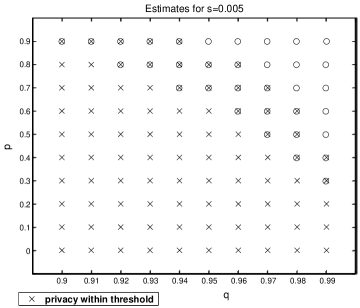
Figure 3: Determining Acceptable $p,q$ Candidates

6 Experimental Results

We evaluated the privacy, accuracy and efficiency of the EMASK privacy-preserving mining process for the candidate distortion parameters on the two datasets for a variety of minimum support values. Due to space limitations, we present here the results only for 0.3% $sup_{min}$ value, which represents a support low enough for a large number of frequent itemsets to be produced, thereby stressing the performance of the EMASK algorithm. The results for the synthetic database are presented first, followed by those for the real database.

6.1 Experiment Set 1 : Synthetic Dataset

Mining the synthetic dataset with a $sup_{min}$ of 0.3 resulted in frequent itemsets of length upto 8. Table 3 presents the EMASK privacy, accuracy and efficiency results for this dataset in a summarized fashion. In this table, for each $p,q$ candidate, BP and RP denote the basic and re-interrogated privacies, respectively; $\Delta$ denotes the slowdown of EMASK; and the remaining columns show the accuracy metrics. We also include the variances (across mining levels) of the accuracy metrics to determine whether the accuracy was skewed based on the lengths of the frequent itemsets.

p	q	BP	RP	$\Delta$	$\sigma^{+}$	$\sigma^{-}$	$\rho$	$Var(\sigma^{+})$	$Var(\sigma^{-})$	$Var(\rho)$
0.6	0.96	92	70	5.2	4.99	5.34	3.39	3.23	6.84	0.27
0.5	0.97	92.6	74	3.8	5.64	6.27	4.86	7.74	6.41	4.31
0.4	0.98	93	78	2.4	6.40	7.87	6.60	6.13	18.35	19.02
0.3	0.99	92.6	80	1.1	6.63	11.69	10.19	7.61	137.20	120.24

Table 3: Performance Results for Synthetic dataset

The first point to note in Table 3 is that the results are very encouraging since they clearly demonstrate that EMASK is able to get high values for all three competing objectives – for example, with $(0.4,0.98)$, the basic and re-interrogated privacy are above 75 percent, the slowdown is only 2.4 (that is, it performed only around twice as slow as Apriori), and the accuracy on all measures is better than 90 percent (less than 10 percent error).

Secondly, note that the $\Delta$ slowdown values across all the combinations is such that EMASK always performs within 5 times of Apriori. This is indeed a huge improvement from the several orders of magnitude inefficiency that was exhibited by MASK, as discussed earlier in Section 4.

Third, while it may appear that $(0.3,0.99)$ is very desirable from privacy and efficiency perspectives (it executes almost as quickly as Apriori and has an 80-plus privacy), yet it may not be a suitable choice since the variance in the accuracy measures is very high. Specifically, the longer (and potentially most important) frequent itemsets have much higher errors with the combinations with low $p$ values like this. Table 4 and Table 5 show errors at each level for ${0.6,0.96}$ (highest $p$ value in the candidates) and ${0.3,0.99}$ (lowest $p$ value) respectively. In the tables, the Level indicates the length of the frequent itemsets, $|F|$ indicates the number of frequent itemset at this level, and other three columns are error metrics as discussed before. The tables indicate that to ensure high accuracy at higher levels one must move to high $p$ values among the candidate combinations.

Level	$|F|$	$\sigma^{+}$	$\sigma^{-}$	$\rho$
1	664	1.5	1.5	3.21
2	1847	5.79	5.46	3.38
3	1310	3.66	4.27	2.9
4	864	7.29	6.13	3.45
5	419	6.2	12.88	4.35
6	115	6.08	4.34	5.44
7	21	4.76	4.76	6.86
8	2	0	0	5.39

Table 4: p=0.6,q=0.96,$\rm{sup_{min}}$=0.3%

Level	$|F|$	$\sigma^{+}$	$\sigma^{-}$	$\rho$
1	664	0.75	1.95	3.11
2	1847	7.95	6.93	5.09
3	1310	7.63	7.63	8.16
4	864	8.91	16.31	14.29
5	419	4.53	35.56	26.18
6	115	0	53.91	46.81
7	21	0	85.71	123.04
8	2	0	100	0

Table 5: p=0.3,q=0.99,$\rm{sup_{min}}$=0.3%

Finally, since no single combination is the best in all respects, the specific tradeoffs between privacy, accuracy and efficiency have to be determined by the service provider to suit her requirements. Among the chosen candidates for $p,q$, moving to higher $p$ values gives better accuracy, moving to lower $p$ values gives better privacy and moving to higher $q$ values gives better efficiency. But,the important point is that no matter which of these combinations is chosen, they all provide 70-plus privacy, 80-plus accuracy, and slowdown less than 5.

6.2 Experiment Set 2: Real Dataset

We conducted a similar set of experiments on the real dataset (BMS-WebView-1 [15]), which had frequent itemsets of length upto 4 for 0.3% minimum support setting. The results for this set of experiments are shown in Table 6.

p	q	BP	RP	$\Delta$	$\sigma^{+}$	$\sigma^{-}$	$\rho$	$Var(\sigma^{+})$	$Var(\sigma^{-})$	$Var(\rho)$
0.8	0.96	92.7	71	4.8	3.21	3.67	3.21	2.34	1.67	0.67
0.7	0.96	94.3	76	4.8	4.13	3.90	3.86	6.45	1.46	0.65
0.6	0.96	95.8	81.4	4.8	5.05	5.28	4.80	11.96	4.47	0.42
0.6	0.97	94.5	78	3.7	4.36	4.36	4.08	10.13	1.47	0.24
0.7	0.97	92.7	73	3.6	2.98	3.67	3.34	3.05	1.67	0.36
0.6	0.98	92.1	74	2.5	3.67	3.67	3.30	3.03	3.21	0.16
0.5	0.98	94.3	79.5	2.4	4.36	4.82	4.35	3.50	11.53	0.20
0.4	0.98	96.2	85.7	2.7	6.43	6.66	5.97	26.63	14.24	0.56
0.4	0.99	93.2	79.3	1.6	5.28	5.05	4.78	15.40	16.50	1.34
0.3	0.99	96	87	1.3	8.96	7.81	6.29	201.96	33.20	1.51

Table 6: Performance Results for Real Dataset

The first point to note in Table 6 is that the privacy and accuracy results are noticeably better than their counterparts in the synthetic dataset experiment. On the other hand, the slowdown values are marginally higher. This is because Apriori is able to take full advantage of the increased sparseness of this dataset, whereas EMASK still has to pay a price for the density increases that are an outcome of the distortion process. Secondly, there are a richer set of tradeoffs that are available to the service provider to suit her requirements. Finally, note again that setting very high values of $q$, specifically $q=0.99$, while very attractive from privacy and efficiency perspectives, results in high variance for the accuracy measures. Here too, the errors are primarily incurred by the longer frequent itemsets.

6.3 Summary

Overall, our experiments indicate that by a careful choice of distortion parameter settings, it is possible to simultaneously achieve satisfactory privacy, accuracy, and efficiency. In particular, they show that there is a “window of opportunity” where these triple goals can be all met. The size and position of the window is primarily a function of the database density and could be quite accurately characterized with our estimation methods.

7 Related Work

The issue of maintaining privacy in association rule mining has attracted considerable attention in the recent past [12, 6, 7, 13, 14, 10, 8, 9]. However, to the best of our knowledge, none of these previous papers have tackled the issue of efficiency in privacy-preserving mining.

The work closest to our approach is that of [8, 9]. A set of randomization operators for maintaining data privacy were presented and analyzed in [8]. New formulations of privacy breaches and a methodology for limiting them were given in [9]. The problem of large transactions resulting from distortion was also mentioned in [9], but they addressed this problem from the perspective of reducing storage and communication costs, but not runtime mining efficiency. Specifically, they proposed a compression technique for reducing the effective size of the distorted database.

Another difference is that EMASK (and MASK) support a notion of “average privacy”, that is, they compute the probability of being able to accurately reconstruct a random entry in the database. In contrast, [8, 9] evaluate the probability of accurately reconstructing a specific entry in the database. In [1], we present a detailed quantitative argument for why it appears fundamentally unlikely that efficient mining algorithms can be designed to support this stronger measure of privacy.

Finally, the problem addressed in [12, 6, 7, 13] is how to prevent sensitive rules from being inferred by the data miner – this work is complementary to ours since it addresses concerns about output privacy, whereas our focus is on the privacy of the input data. Maintaining input data privacy is considered in [14, 10] in the context of databases that are distributed across a number of sites with each site only willing to share data mining results, but not the source data.

8 Conclusions

In this paper, we have considered, for the first time, the issue of providing efficiency in privacy-preserving mining. Our goal was to investigate the possibility of simultaneously achieving high privacy, accuracy and efficiency in the mining process. We first showed how the distortion process required for ensuring privacy can have a marked negative side-effect of hugely increasing mining runtimes. Then, we presented our new EMASK algorithm that is specifically designed to minimize this side-effect through the application of symbol-specific distortion. We derived simple but effective formulas for estimating acceptable settings of the distortion parameters. We also presented a simple but powerful optimization by which all additional counting incurred by privacy preserving mining is moved to the end of each pass over the database.

Our experiments show that EMASK exploits a small window of opportunity around the distortion combination ($p=0.4,q=0.98$) which can simultaneously provide good privacy, accuracy and efficiency. Specifically, less than 5 times slowdown with respect to Apriori in conjunction with 70-plus privacies and 80-plus accuracies, were achieved with these settings. In summary, EMASK takes a significant step towards making privacy-preserving mining of association rules a viable enterprise.

References

- [1] S. Agrawal, V. Krishnan and J. Haritsa, “Providing Efficiency in Privacy-Preserving Mining”, Tech. Rep. 2003-02, DSL/SERC, Indian Institute of Science, August 2003.
- [2] D. Agrawal and C. Aggarwal, “On the Design and Quantification of Privacy Preserving Data Mining Algorithms”, Proc. of 20th ACM Symp. on Principles of Database Systems (PODS), May 2001.
- [3] R. Agrawal, T. Imielinski and A. Swami, “Mining association rules between sets of items in large databases”, Proc. of ACM SIGMOD Intl. Conference on Management of Data (SIGMOD), May 1993.
- [4] R. Agrawal and R. Srikant, “Fast algorithms for mining association rules”, Proc. of 20th Intl. Conf. on Very Large Data Bases (VLDB), September 1994.
- [5] R. Agrawal and R. Srikant, “Privacy-Preserving Data Mining”, Proc. of ACM SIGMOD Intl. Conf. on Management of Data, May 2000.
- [6] M. Atallah, E. Bertino, A. Elmagarmid, M. Ibrahim and V. Verykios, “Disclosure Limitation of Sensitive Rules”, Proc. of IEEE Knowledge and Data Engineering Exchange Workshop (KDEX), November 1999.
- [7] E. Dasseni, V. Verykios, A. Elmagarmid and E. Bertino, “Hiding Association Rules by Using Confidence and Support”, Proc. of 4th Intl. Information Hiding Workshop (IHW), April 2001.
- [8] A. Evfimievski, R. Srikant, R. Agrawal and J. Gehrke, “Privacy Preserving Mining of Association Rules”, Proc. of 8th ACM SIGKDD Intl. Conf. on Knowledge Discovery and Data Mining (KDD), July 2002.
- [9] A. Evfimievski, J. Gehrke and R. Srikant, ”Limiting Privacy Breaches in Privacy Preserving Data Mining”, Proc. of ACM Symp. on Principles of Database Systems, June 2003.
- [10] M. Kantarcioglu and C. Clifton, “Privacy-preserving Distributed Mining of Association Rules on Horizontally Partitioned Data”, Proc. of ACM SIGMOD Workshop on Research Issues in Data Mining and Knowledge Discovery (DMKD), June 2002.
- [11] S. Rizvi and J. Haritsa, ”Maintaining Data Privacy in Association Rule Mining”, Proc. of 28th Intl. Conf. on Very Large Databases (VLDB), August 2002.
- [12] Y. Saygin, V. Verykios and C. Clifton, “Using Unknowns to Prevent Discovery of Association Rules”, ACM SIGMOD Record, vol. 30, no. 4, 2001.
- [13] Y. Saygin, V. Verykios and A. Elmagarmid, “Privacy Preserving Association Rule Mining”, Proc. of 12th Intl. Workshop on Research Issues in Data Engineering (RIDE), February 2002.
- [14] J. Vaidya and C. Clifton, “Privacy Preserving Association Rule Mining in Vertically Partitioned Data”, Proc. of 8th ACM SIKGDD Intl. Conference on Knowledge Discovery and Data Mining (KDD), July 2002.
- [15] Z. Zheng, R. Kohavi and L. Mason, “Real World Performance of Association Rule Algorithms”, Proc. of 7th ACM SIGKDD Intl. Conference on Knowledge Discovery and Data Mining (KDD), August 2001.