Maximum Dispersion
and Geometric Maximum Weight Cliques

Abstract

We consider a facility location problem, where the objective is to “disperse” a number of facilities, i.e., select a given number $k$ of locations from a discrete set of $n$ candidates, such that the average distance between selected locations is maximized. In particular, we present algorithmic results for the case where vertices are represented by points in $d$-dimensional space, and edge weights correspond to rectilinear distances. Problems of this type have been considered before, with the best result being an approximation algorithm with performance ratio 2. For the case where $k$ is fixed, we establish a linear-time algorithm that finds an optimal solution. For the case where $k$ is part of the input, we present a polynomial-time approximation scheme.

1 Introduction

A common problem in the area of facility location is the selection of a given number of $k$ locations from a set $P$ of $n$ feasible positions, such that the selected set has optimal distance properties. Natural objective functions are the maximization of the minimum distance, or of the average distance between selected points; dispersion problems of this type come into play whenever we want to minimize interference between the corresponding facilities. Examples include oil storage tanks, ammunition dumps, nuclear power plants, hazardous waste sites, and fast-food outlets (see [14, 5]). In the latter paper, the problem of maximizing the average distance is called the Remote Clique problem.

Formally, problems of this type can be described as follows: given a graph $G=(V,E)$ with $n$ vertices, and non-negative edge weights $w_{v_{1},v_{2}}=d(v_{1},v_{2})$ for $(v_{1},v_{2})\in E$. Given $k\in\{2,\ldots,n\}$, find a subset $S\subset V$ with $|S|=k$, such that $w(S):=\sum_{(v_{i},v_{j})\in E(S)}d(v_{i},v_{j})$ is maximized. (Here, $E(S)$ denotes the edge set of the subgraph of $G$ induced by the vertex set $S$.)

From a graph theoretic point of view, this problem has been called a heaviest subgraph problem. Being a weighted version of a generalization of the problem of deciding the existence of a $k$-clique, i.e., a complete subgraph with $k$ vertices, the problem is strongly NP-hard [16]. It should be noted that Håstad [11] showed that the problem Clique of maximizing the cardinality of a set of vertices with a maximum possible number of edges is in general hard to approximate within $n^{1-\varepsilon}$. For the heaviest subgraph problem, we want to maximize the number of edges for a set of vertices of given cardinality, so Håstad’s result does not imply an immediate performance bound.

Related Work

Over recent years, there have been a number of approximation algorithms for various subproblems of this type. Feige and Seltser [7] have studied the graph problem (i.e., edge weights are $0$ or $1$) and showed how to find in time $n^{O((1+\log\frac{n}{k})/\varepsilon)}$ a $k$-set $S\subset V$ with $w(S)\geq(1-\varepsilon)\left(\begin{array}[]{c}k\\ 2\end{array}\right)$, provided that a $k$-clique exists. They also gave evidence that for $k\simeq n^{1/3}$, semidefinite programming fails to distinguish between graphs that have a $k$-clique, and graphs with densest $k$-subgraphs having average degree less than $\log n$.

Kortsarz and Peleg [12] describe a polynomial algorithm with performance guarantee $O(n^{0.3885})$ for the general case where edge weights do not have to obey the triangle inequality. A newer algorithm by Feige, Kortsarz, and Peleg [8] gives an approximation ratio of $O(n^{1/3}\log n)$. For the case where $k=\Omega(n)$, Asahiro, Iwama, Tamaki, and Tokuyama [3] give a greedy constant factor approximation, while Srivastav and Wolf [15] use semidefinite programming for improved performance bounds. For the case of dense graphs (i.e., $|E|=\Omega(n^{2})$) and $k=\Omega(n)$, Arora, Karger, and Karpinski [1] give a polynomial time approximation scheme. On the other hand, Asahiro, Hassin, and Iwama [2] show that deciding the existence of a “slightly dense” subgraph, i.e., an induced subgraph on $k$ vertices that has at least $\Omega(k^{1+\varepsilon})$ edges, is NP-complete. They also showed it is NP-complete to decide whether a graph with $e$ edges has an induced subgraph on $k$ vertices that has $\frac{ek^{2}}{n^{2}}(1+O(v^{\varepsilon-1}))$ edges; the latter is only slightly larger than $\frac{ek^{2}}{n^{2}}(1-\frac{v-k}{vk-k})$, which is the the average number of edges in a subgraph with $k$ vertices.

For the case where edge weights fulfill the triangle inequality, Ravi, Rosenkrantz, and Tayi [14] give a heuristic with time complexity $O(n^{2})$ and prove that it guarantees a performance bound of 4. (See Tamir [17] with reference to this paper.) Hassin, Rubinstein, and Tamir [10] give a different heuristic with time complexity $O(n^{2}+k^{2}\log k)$ with performance bound 2. On a related note, see Chandra and Halldórsson [5], who study a number of different remoteness measures for the subset $k$, including total edge weight $w(S)$. If the graph from which a subset of size $k$ is to be selected is a tree, Tamir [16] shows that an optimal weight subset can be determined in $O(nk)$ time.

In many important cases there is even more known about the set of edge weights than just the validity of triangle inequality. This is the case when the vertex set $V$ corresponds to a point set $P$ in geometric space, and distances between vertices are induced by geometric distances between points. Given the practical motivation for considering the problem, it is quite natural to consider geometric instances of this type. In fact, it was shown by Ravi, Rosenkrantz, and Tayi in [14] that for the case of Euclidean distances in two-dimensional space, it is possible to achieve performance bounds that are arbitrarily close to $\pi/2\approx 1.57$ For other metrics, however, the best performance guarantee is the factor 2 by [10]. Despite of these approximation results, it should be noted that the complexity status of the problem is still open, i.e., it is known known whether the problem is NP-hard.

An important application of our problem is data sampling and clustering, where points are to be selected from a large more-dimensional set. Different metric dimensions of a data point describe different metric properties of a corresponding item. Since these properties are not geometrically related, distances are typically not evaluated by Euclidean distances. Instead, some weighted $L_{1}$ metric is used. (See Erkut [6].) For data sampling, a set of points is to be selected that has high average distance. For clustering, a given set of points is to be subdivided into $k$ clusters, such that points from the same cluster are close together, while points from different clusters are far apart. If we do the clustering by choosing $k$ center points, and assigning any point to its nearest cluster center, we have to consider the same problem of finding a set of center points with large average distance, which is equivalent to finding a $k$-clique with maximum total edge weight.

For results on maximizing the minimum $L_{1}$ distance within a selected set of $n$ points see Baur and Fekete  [4], who showed that finding such a set within a given polygon cannot be approximated arbitrarily well, unless P=NP. Finally, Gritzmann, Klee, and Larmann [9] have studied a somewhat related geometric selection problem: Given a set $v$ of $m$ points in $n$-dimensional space, choose a subset of $n+1$ points, such that the total volume of the resulting simplex is maximum. They showed that this problem is NP-hard when $n$ is part of the input.

Main Results

In this paper, we consider point sets $P$ in $d$-dimensional space, where $d$ is some constant. For the most part, distances are measured according to the rectilinear “Manhattan” norm $L_{1}$.

Our results include the following:

• A linear time $(O(n))$ algorithm to solve the problem to optimality in case where $k$ is some fixed constant. This is in contrast to the case of Euclidean distances, where there is a well-known lower bound of $\Omega(n\log n)$ in the computation tree model for determining the diameter of a planar point set, i.e., the special case $d=2$ and $k=2$ (see [13]).

• A polynomial time approximation scheme for the case where $k$ is not fixed. This method can be applied for arbitrary fixed dimension $d$. For the case of Euclidean distances in two-dimensional space, it implies a performance bound of $\sqrt{2}+\varepsilon$, for any given $\varepsilon>0$.

2 Preliminaries

For the most part of this paper, all points are assumed to be points in the plane. Spaces of arbitrary fixed dimension will be discussed in the end. Distances are measured using the $L_{1}$ norm, unless noted otherwise. The $x$- and $y$-coordinates of a point $p$ are denoted by $x_{p}$ and $y_{p}$. If $p$ and $q$ are two points in the plane, then the distance between $p$ and $q$ is $d(p,q)=|x_{p}-x_{q}|+|y_{p}-y_{q}|$. We say that $q$ is above $p$ in direction of a vector $c$, if the inner products satisfy $\langle q,c\rangle\geq\langle p,c\rangle$ We say that a point $p$ is maximal in direction $c$ with respect to a set of points $P$ if it maximizes the inner product $\{\langle c,x\rangle\mid x\in P\}$. For example, if $p$ is an element of a set of points $P$ and $p$ has a maximal $y$-coordinate, then $p$ is maximal in direction (0,1) with respect to $P$, and a point $p$ with minimal $x$-coordinate is maximal in direction (-1,0) with respect to $P$. If the set $P$ is clear from the context, we simply state that $p$ is maximal in direction $c$.

The weight of a set of points $P$ is the sum of the distances between all pairs of points in this set, and is denoted by $w(P)$. Similarly, $w(P,Q)$ denotes the total sum of distances between two sets $P$ and $Q$. For $L_{1}$ distances, $w_{x}(P)$ and $w_{x}(P,Q)$ denote the sum of $x$-distances within $P$, or between $P$ and $Q$.

3 Cliques of Fixed Size

Let $S=\{s_{0},s_{1},\ldots,s_{k-1}\}$ be a maximum weight subset of $P$, where $k$ is a fixed integer greater than 1. We will label the $x$- and $y$-coordinates of a point $s\in S$ by some $(x_{a},y_{b})$ with $0\leq a<k$ and $0\leq b<k$ such that $x_{0}\leq x_{1}\leq\ldots\leq x_{k-1}$ and $y_{0}\leq y_{1}\leq\ldots\leq y_{k-1}$. (Note that in general, $a\neq b$ for a point $s=(x_{a},y_{b})$.) Then

$$w(S)\leavevmode\nobreak\ =\leavevmode\nobreak\ \sum_{0\leq i<j<k}(x_{j}-x_{i})+\sum_{0\leq i<j<k}(y_{j}-y_{i}).$$

Now we can use local optimality to reduce the family of subsets that we need to consider:

Lemma 1

There is a maximum weight subset $S^{\prime}$ of $P$ of cardinality $k$, such that each point in $S^{\prime}$ is maximal in direction $(2i+1-k,2j+1-k)$ with respect to $P\setminus S^{\prime}$ for some values of $i$ and $j$ with $0\leq i,j<k$.

Proof: Consider a maximum weight subset $S\subset P$ of cardinality $k$. Let $s=(x_{i},y_{i^{\prime}})$ be a point in $S$, such that there are $i$ points $s_{l}=(x_{l},y_{l^{\prime}})\in S\setminus\{s\}$ with $x_{l}\leq x_{i}$ (i.e., to the left of $s$) and $k-i-1$ points $s_{l}=(x_{l},y_{l^{\prime}})\in S\setminus\{s\}$ with $x_{l}>x_{i}$ (i.e., strictly to the right of $s$). Similarly let there be $j$ points below $s$ and $k-j-1$ points strictly above $s$. We claim that $s$ is maximal in direction $(2i+1-k,2j+1-k)$ with respect to $P-S$.

Consider replacing $s$ by a point $s^{\prime}=s+(x_{h},y_{h})$ in $P-S$. Let $\delta=(2i+1-k)x_{h}+(2j+1-k)y_{h}$. Let $S^{\prime}=S\setminus\{s\}\cup\{s^{\prime}\}$. Assume first that point $s^{\prime}=(x_{i}^{\prime},y_{i^{\prime}}^{\prime})$ is such that $x_{i}^{\prime}$ and $y_{i^{\prime}}^{\prime}$ have the same rank in $S^{\prime}$ as $x_{i}$ and $y_{i^{\prime}}$ have in $S$, i.e., there are $i$ points $s_{l}=(x_{l},y_{l})\in S^{\prime}\setminus\{s^{\prime}\}$ with $x_{l}\leq x_{i}^{\prime}$ and $j$ points $s_{l}=(x_{l},y_{l^{\prime}})\in S^{\prime}\setminus\{s^{\prime}\}$ with $y_{l^{\prime}}\leq y_{i^{\prime}}^{\prime}$. Replacing $s$ by $s^{\prime}$ changes the $x$-distances to the points left of $s$ by $ix_{h}$, and the $x$-distances to the points right of $s$ by $(k-i-1)(-x_{h})$. Similarly, the $y$-distances change by $jy_{h}$ and $(k-j-1)y_{h}$. So $w(S^{\prime})=w(S)+(2i+1-k)x_{h}+(2j+1-k)y_{h}=w(S)+\delta$. Since $w(S)$ is maximum, we derive that $\delta\leq 0$, i.e., no point in $P-S$ is above any point in $S$ in direction $(2i+1-k,2j+1-k)$.

If the $x$- and $y$-coordinates of $s^{\prime}$ do not have the same rank in $S^{\prime}$ as the $x$- and $y$-coordinates of $s$ in $S$, then it is not hard to show that $w(S^{\prime})>w(S)+\delta$, so $\delta<0$. Therefore in this case, $s^{\prime}$ is strictly below $s$ in direction $(2i+1-k,2j+1-k)$.

We can also conclude that if $s=(x_{i},y_{i^{\prime}})$ and $s^{\prime}=(x_{i}^{\prime},y_{i^{\prime}}^{\prime})$ are at the same level in direction $(2i+1-k,2j+1-k)$, i.e., if $\delta=0$, then the $x$- and $y$-coordinates of $s^{\prime}$ do have the same rank in $S^{\prime}$ as the $x$- and $y$-coordinates of $s$ in $S$ and $w(S)=w(S^{\prime})$. $\Box$

Theorem 1

Given a constant value for $k$, a maximum weight subset $S$ of a set of $n$ points $P$, such that $S$ has cardinality $k$, can be found in linear time.

Proof: Consider all directions of the form $(2i+1-k,2j+1-k)$ with $0\leq i,j<k$. For each direction $(a,b)$, find $S_{k}(a,b)$, a set of $k$ points that are maximal in direction $(a,b)$ with respect to $P-S_{k}(a,b)$. Compute the set $\cup S_{k}(a,b)$ and try all possible subsets of size $k$ of this set until a subset of maximum weight is found.

Correctness follows from the fact that Lemma 1 implies that $S\subset\cup S_{k}(a,b)$. Since $k$ is a constant, each set $S_{k}(a,b)$ can be found in linear time. Since the cardinality of $\cup S_{k}(a,b)$ is less than or equal to $k^{3}$, the result follows. From the discussion at the end of the proof of Lemma 1 we can conclude that if the set of $k$ points maximal in a direction $(a,b)$ is not unique, any set of $k$ points maximal in this direction will work equally well.

$\Box$

Note that in the above estimate, we did not try to squeeze the constants in the $O(n)$ running time. A closer look shows that for $k=2$, not more than $2$ subsets of $P$ need to be evaluated for possible optimality, for $k=3$, 8 subsets are sufficient.

4 Cliques of Variable Size

In this section we consider the scenario where $k$ is not fixed, i.e., $k$ is part of the input. We show that there is a polynomial time approximation scheme (PTAS), i.e., for any fixed positive $\varepsilon$, there is a polynomial approximation algorithm that finds a solution that is within $(1+\varepsilon)$ of the optimum.

The basic idea is to use for each of the $d$ coordinates a suitable subset of $m_{\varepsilon}$ coordinate values that subdivide an optimal solution into subsets of equal cardinality. More precisely, we describe the case $d=2$; we find (by enumeration) a subdivision of an optimal solution into $m_{\varepsilon}\times m_{\varepsilon}$ rectangular cells $C_{ij}$, each of which must contain a specific number $k_{ij}$ of selected points. From each cell $C_{ij}$, the points are selected in a way that guarantees that the total distance to all other cells except for the $m_{\varepsilon}-1$ cells in the same “horizontal” strip or the $m_{\varepsilon}-1$ cells in the same “vertical” strip is maximized. As it turns out, this can be done in a way that the total neglected distance within the strips is bounded by a fraction of $(5m_{\varepsilon}-9)/(2(m_{\varepsilon}-1)(m_{\varepsilon}-2))$ of the weight of an optimal solution, yielding the desired approximation property. See Figure 1 for the overall picture.

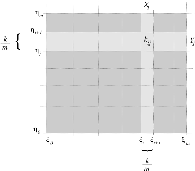
Figure 1: Subdividing the plane into cells

For ease of presentation we assume that $k$ is a multiple of $m_{\varepsilon}$ and $m_{\varepsilon}>2$. Approximation algorithms for other values of $k$ can be constructed in a similar fashion. Consider an optimal solution of $k$ points, denoted by OPT. Furthermore consider a division of the plane by a set of $m_{\varepsilon}+1$ $x$-coordinates $\xi_{0}\leq\ldots\leq\xi_{1}\leq\xi_{m_{\varepsilon}}$. Let $X_{i}:=\{p=(x,y)\in\Re^{2}\mid\xi_{i}\leq x\leq\xi_{i+1},0\leq i<m_{\varepsilon}\}$ be the vertical strip between coordinates $\xi_{i}$ and $\xi_{i+1}$. By enumeration of possible choices of $\xi_{0},\ldots,\xi_{m_{\varepsilon}}$ we may assume that the $\xi_{i}$ have the property that, for an optimal solution, from each of the $m_{\varepsilon}$ strips $X_{i}$ precisely $k/m_{\varepsilon}$ points of $P$ are chosen. (A small perturbation does not change optimality or approximation properties of solutions. This shows that in case of several points sharing the same coordinates, ties may be broken arbitrarily; in that case, points on the boundary between two strips may be considered belonging to one or the other of those strips, whatever is convenient to reach the appropriate number of points in a strip.)

In a similar manner, suppose we know $m_{\varepsilon}+1$ $y$-coordinates $\eta_{0}\leq\eta_{1}\leq\ldots\leq\eta_{m_{\varepsilon}}$ such that from each horizontal strip $Y_{i}:=\{p=(x,y)\in\Re^{2}\mid\eta_{i}\leq y\leq\eta_{i+1},0\leq i<m_{\varepsilon}\}$ a subset of $k/m_{\varepsilon}$ points are chosen for an optimal solution.

Let $C_{ij}:=X_{i}\cap Y_{j}$, and let $k_{ij}$ be the number of points in OPT that are chosen from $C_{ij}$. Since $\sum_{0\leq i<m_{\varepsilon}}k_{ij}=\sum_{0\leq j<m_{\varepsilon}}k_{ij}=k/m_{\varepsilon}$, we may assume by enumeration over the $O(k^{m}_{\varepsilon})$ possible partitions of $k/m_{\varepsilon}$ into $m_{\varepsilon}$ pieces that we know all the numbers $k_{ij}$.

Finally, define the vector $\nabla_{ij}:=((2i+1-m_{\varepsilon})k/m_{\varepsilon},(2j+1-m_{\varepsilon})k/m_{\varepsilon})$. Now our approximation algorithm is as follows: from each cell $C_{ij}$, choose some $k_{ij}$ points that are maximal in direction $\nabla_{ij}$. (Overlap between the selections from different cells is avoided by proceeding in lexicographic order of cells, and choosing the $k_{ij}$ points among the candidates that are still unselected.) Let HEU be the point set selected in this way.

It is clear that HEU can be computed in polynomial time. We will proceed by a series of lemmas to determine how well $w(\mbox{\it HEU})$ approximates $w(\mbox{\it OPT})$. In the following, we consider the distances involving points from a particular cell $C_{ij}$. Let $\mbox{\it HEU}_{ij}$ be the set of $k_{ij}$ points that are selected from $C_{ij}$ by the heuristic, and let $\mbox{\it OPT}_{ij}$ be a set of $k_{ij}$ points of an optimal solution that are attributed to $C_{ij}$. Let $S_{ij}=\mbox{\it OPT}_{ij}\cap\mbox{\it HEU}_{ij}$. Furthermore we define $\overline{S}_{ij}=\mbox{\it HEU}_{ij}\setminus\mbox{\it OPT}_{ij}$, and $\tilde{S}_{ij}=\mbox{\it OPT}_{ij}\setminus\mbox{\it HEU}_{ij}$. Let $\mbox{\it HEU}_{i\bullet}$, $\mbox{\it OPT}_{i\bullet}$, $\mbox{\it HEU}_{\bullet j}$ and $\mbox{\it OPT}_{\bullet j}$ be the set of $k/m_{\varepsilon}$ points selected from $X_{i}$ and $Y_{j}$ by the heuristic and an optimal algorithm respectively. Finally $\overline{\mbox{\it HEU}}_{i\bullet}:=\mbox{\it HEU}\setminus\mbox{\it HEU}_{i\bullet}$, $\overline{\mbox{\it HEU}}_{\bullet j}:=\mbox{\it HEU}\setminus\mbox{\it HEU}_{\bullet j}$, $\overline{\mbox{\it OPT}}_{i\bullet}:=\mbox{\it OPT}\setminus\mbox{\it OPT}_{i\bullet}$ and $\overline{\mbox{\it OPT}}_{\bullet j}:=\mbox{\it OPT}\setminus\mbox{\it OPT}_{\bullet j}$.

Lemma 2

$$w_{x}(\mbox{\it HEU}_{ij},\overline{\mbox{\it HEU}}_{i\bullet})+w_{y}(\mbox{\it HEU}_{ij},\overline{\mbox{\it HEU}}_{\bullet j})$$

$$\geq w_{x}(\mbox{\it OPT}_{ij},\overline{\mbox{\it OPT}}_{i\bullet})+w_{y}(\mbox{\it OPT}_{ij},\overline{\mbox{\it OPT}}_{\bullet j}).$$

Proof: Consider a point $p\in\tilde{S}_{ij}$. Thus, there is a point $p^{\prime}\in\overline{S}_{ij}$ that was chosen by the heuristic instead of $p$. Now we can argue like in Lemma 1: Let $h=(h_{x},h_{y})=p^{\prime}-p$. When replacing $p$ in OPT by $p^{\prime}$, we increase the $x$-distance to the $ik/m_{\varepsilon}$ points “left” of $C_{ij}$ by $h_{x}$, while decreasing the $x$-distance to $(m_{\varepsilon}-i-1)k/m_{\varepsilon}$ points “right” of $C_{ij}$ by $h_{x}$. In the balance, this yields a change of $((2i+1-m_{\varepsilon})k/m_{\varepsilon})h_{x}$. Similarly, we get a change of $((2j+1-m_{\varepsilon})k/m_{\varepsilon})h_{y}$ for the $y$-coordinates. By definition, we have assumed that the inner product $\langle h,\nabla_{ij}\rangle\geq 0$, so the overall change of distances is nonnegative.

Performing these replacements for all points in $\mbox{\it OPT}\setminus\mbox{\it HEU}$, we can transform OPT to HEU, while increasing the sum of distances $w_{x}(\mbox{\it OPT}_{ij},\overline{\mbox{\it OPT}}_{i\bullet})+w_{y}(\mbox{\it OPT}_{ij},\overline{\mbox{\it OPT}}_{\bullet j})$ to the sum $w_{x}(\mbox{\it HEU}_{ij},\overline{\mbox{\it HEU}}_{i\bullet})+w_{y}(\mbox{\it HEU}_{ij},\overline{\mbox{\it HEU}}_{\bullet j})$.

$\Box$

In the following three lemmas we show that the total difference between the weight of an optimal solution $w(\mbox{\it OPT})$ and the total value of all the right hand sides (when summed over $i$) of the inequality in Lemma 2 is a small fraction of $w(\mbox{\it OPT})$.

Lemma 3

$$\sum_{0<i<m_{\varepsilon}-1}w_{x}(\mbox{\it OPT}_{i\bullet})\leavevmode\nobreak\ \leq\leavevmode\nobreak\ \frac{w_{x}(\mbox{\it OPT})}{2(m_{\varepsilon}-2)}.$$

Proof: Let $\delta_{i}=\xi_{i+1}-\xi_{i}$. Since $i(m_{\varepsilon}-i-1)\geq m_{\varepsilon}-2$ for $0<i<m_{\varepsilon}-1$, we have for $0<i<m_{\varepsilon}-1$

$$w_{x}(\mbox{\it OPT}_{i\bullet})\leq\frac{k^{2}}{2m_{\varepsilon}^{2}}\delta_{i}\leq\frac{ik}{m_{\varepsilon}}\frac{(m_{\varepsilon}-i-1)k}{m_{\varepsilon}}\delta_{i}\leavevmode\nobreak\ \frac{1}{2(m_{\varepsilon}-2)}.$$

Since OPT has $ik/m_{\varepsilon}$ and $(m_{\varepsilon}-i-1)k/m_{\varepsilon}$ points to the left of $\xi_{i}$ and right of $\xi_{i+1}$ respectively, we have

$$w_{x}(\mbox{\it OPT})\geq\sum_{0<i<m_{\varepsilon}-1}\frac{ik}{m_{\varepsilon}}\frac{(m_{\varepsilon}-i-1)k}{m_{\varepsilon}}\delta_{i}$$

so

$$\sum_{0<i<m_{\varepsilon}-1}w_{x}(\mbox{\it OPT}_{i\bullet})\leq\frac{1}{2(m_{\varepsilon}-2)}w_{x}(\mbox{\it OPT}).$$

$\Box$

Lemma 4

For $i=0$ and $i=m_{\varepsilon}-1$ we have

$$w_{x}(\mbox{\it OPT}_{i\bullet})\leavevmode\nobreak\ \leq\leavevmode\nobreak\ \frac{w_{x}(\mbox{\it OPT})}{m_{\varepsilon}-1}$$

Proof: Without loss of generality assume $i=0$. Let $x_{0},x_{1},\cdots,x_{(k/m_{\varepsilon})-1}$ be the $x$-coordinates of the points $p_{0},p_{1},\ldots,p_{(k/m_{\varepsilon})-1}$ in $\mbox{\it OPT}_{0\bullet}$. So

$$w_{x}(\mbox{\it OPT}_{0\bullet})\leavevmode\nobreak\ =\leavevmode\nobreak\ (\frac{k}{m_{\varepsilon}}-1)(x_{\frac{k}{m_{\varepsilon}}-1}-x_{0})+(\frac{k}{m_{\varepsilon}}-3)(x_{\frac{k}{m_{\varepsilon}}-2}-x_{1})+\leavevmode\nobreak\ \ldots$$

$$\leq(\frac{k}{m_{\varepsilon}}-1)(\xi_{1}-x_{0})+(\frac{k}{m_{\varepsilon}}-3)(\xi_{1}-x_{1})+\leavevmode\nobreak\ \ldots$$

$$\leq\frac{k}{m_{\varepsilon}}(\xi_{1}-x_{0})+\frac{k}{m_{\varepsilon}}(\xi_{1}-x_{1})+\leavevmode\nobreak\ \ldots$$

Since $\xi_{1}-x_{j}\leq x-x_{j}$ where $0\leq j<k/m_{\varepsilon}$ and $x$ is the $x$-coordinate of any point in $\overline{\mbox{\it OPT}}_{0\bullet}$ and since there are $(m_{\varepsilon}-1)k/m_{\varepsilon}$ points in $\overline{\mbox{\it OPT}}_{0\bullet}$, we have

$$\xi_{1}-x_{j}<\frac{m_{\varepsilon}}{(m_{\varepsilon}-1)k}w_{x}(p_{j},\overline{\mbox{\it OPT}}_{0\bullet})$$

so

$$w_{x}(\mbox{\it OPT}_{0\bullet}) \leq \frac{k}{m_{\varepsilon}}\frac{m_{\varepsilon}}{(m_{\varepsilon}-1)k}\sum_{0\leq i<\frac{k}{2m_{\varepsilon}}}w_{x}(p_{i},\overline{\mbox{\it OPT}}_{0\bullet})$$

$$\leq \frac{1}{m_{\varepsilon}-1}\sum_{0\leq i<\frac{k}{m_{\varepsilon}}}w_{x}(p_{i},\overline{\mbox{\it OPT}}_{0\bullet})$$

$$= \frac{1}{m_{\varepsilon}-1}w_{x}(\mbox{\it OPT}_{0\bullet},\overline{\mbox{\it OPT}}_{0\bullet})$$

$$\leq \frac{1}{m_{\varepsilon}-1}w_{x}(\mbox{\it OPT}).$$

$\Box$

This proves the main properties. Now we only have to combine the above estimates to get an overall performance bound:

Lemma 5

$$\sum_{0\leq i<m_{\varepsilon}}w_{x}(\mbox{\it OPT}_{i\bullet},\overline{\mbox{\it OPT}}_{i\bullet})+\sum_{0\leq j<m_{\varepsilon}}w_{y}(\mbox{\it OPT}_{\bullet j},\overline{\mbox{\it OPT}}_{\bullet j})$$

$$\geq(1-\frac{5m_{\varepsilon}-9}{2(m_{\varepsilon}-1)(m_{\varepsilon}-2)})w(\mbox{\it OPT})).$$

Proof: From Lemmas 3 (applied for indices $0<i<m-1$) and 4 (applied twice, once for $i=0$, and once for $i=m-1$), we derive that

$$\sum_{0\leq i<m_{\varepsilon}}w_{x}(\mbox{\it OPT}_{i\bullet})\leavevmode\nobreak\ \leq\leavevmode\nobreak\ \frac{5m_{\varepsilon}-9}{2(m_{\varepsilon}-1)(m_{\varepsilon}-2)}w_{x}(\mbox{\it OPT})$$

and similarly

$$\sum_{0\leq i<m_{\varepsilon}}w_{y}(\mbox{\it OPT}_{\bullet j})\leavevmode\nobreak\ \leq\leavevmode\nobreak\ \frac{5m_{\varepsilon}-9}{2(m_{\varepsilon}-1)(m_{\varepsilon}-2)}w_{y}(\mbox{\it OPT}).$$

Since

$$w(\mbox{\it OPT}) = w_{x}(\mbox{\it OPT})+w_{y}(\mbox{\it OPT})$$

$$= \ \ \ \sum_{0\leq i<m_{\varepsilon}}w_{x}(\mbox{\it OPT}_{i\bullet},\overline{\mbox{\it OPT}}_{i\bullet})+\sum_{0\leq i<m_{\varepsilon}}w_{x}(\mbox{\it OPT}_{i\bullet})$$

$$+\sum_{0\leq j<m_{\varepsilon}}w_{y}(\mbox{\it OPT}_{\bullet j},\overline{\mbox{\it OPT}}_{\bullet j})+\sum_{0\leq j<m_{\varepsilon}}w_{y}(\mbox{\it OPT}_{\bullet j}),$$

the result follows. $\Box$

Putting together Lemma 2 and the error estimate from Lemma 5, the approximation theorem can now be proven.

Theorem 2

For any fixed $m$, HEU can be computed in polynomial time, and

$$w(\mbox{\it HEU})\geq(1-\frac{5m_{\varepsilon}-9}{2(m_{\varepsilon}-1)(m_{\varepsilon}-2)})w(\mbox{\it OPT}).$$

The running time is exponential in $\frac{1}{\varepsilon}$.

Proof: The claim about the running time is clear. (The only step that is exponential in $\frac{1}{\varepsilon}$ is the enumeration over all $O(k^{m_{\varepsilon}})$ possible partitions of $k/m_{\varepsilon}$ into $m_{\varepsilon}$ pieces.) Using Lemmas 2 and 5 we derive

$$w(\mbox{\it HEU})\geq\sum_{0\leq i<m_{\varepsilon}}w_{x}(\mbox{\it HEU}_{i\bullet},\overline{\mbox{\it HEU}}_{i\bullet})+\sum_{0\leq j<m_{\varepsilon}}w_{y}(\mbox{\it HEU}_{\bullet j},\overline{\mbox{\it HEU}}_{\bullet j})$$

$$\geq\sum_{0\leq i<m_{\varepsilon}}w_{x}(\mbox{\it OPT}_{i\bullet},\overline{\mbox{\it OPT}}_{i\bullet})+\sum_{0\leq j<m_{\varepsilon}}w_{y}(\mbox{\it OPT}_{\bullet j},\overline{\mbox{\it OPT}}_{\bullet j})$$

$$\geq(1-\frac{5m_{\varepsilon}-9}{2(m_{\varepsilon}-1)(m_{\varepsilon}-2)})w(\mbox{\it OPT}).$$

$\Box$

5 Implications

It is straightforward to modify our above arguments to point sets under $L_{1}$ distances in an arbitrary $d$-dimensional space, with fixed $d$.

Theorem 3

Given a constant value for $k$ and $d$, a maximum weight subset $S$ of a set of $n$ points in $d$-dimensional space, such that $S$ has cardinality $k$, can be found in linear time. If $d$ and $\varepsilon$ are constants, but $k$ is not fixed, then there is a polynomial time algorithm that finds a subset whose weight is within $(1+\varepsilon)$ of the optimum.

For the case of fixed $k$, it is straightforward to generalize the argument from Section 3 to see that there are at most $(2k)^{d}$ interesting directions to consider. For $k$ being part of the input, the approximation scheme can be generalized in a straightforward manner by using an $m_{\varepsilon}$-subdivision in each coordinate direction. Again the complexity ends up being exponential in $\frac{1}{\varepsilon}$, as well as in $d$.

For the case of $L_{\infty}$ distances in the plane, the results for $L_{1}$ distances can be applied by a standard argument: A rotation by $\pi/4$ transforms $L_{\infty}$ distances into $L_{1}$ distances and vice versa. Furthermore, we can use the approximation scheme from the previous section to get a $\sqrt{2}(1+\varepsilon)$ approximation factor for the case of Euclidean distances in two-dimensional space, for any $\varepsilon>0$: In polynomial time, find a $k$-set $S_{1}$ such that $L_{1}(S)$ is within $(1+\varepsilon)$ of an optimal solution $\mbox{\it OPT}_{1}$ with respect to $L_{1}$ distances. Let $\mbox{\it OPT}_{2}$ be an optimal solution with respect to $L_{2}$ distances. Then

$$L_{2}(S) \geq \frac{1}{\sqrt{2}}L_{1}(S)\geq\frac{1}{\sqrt{2}(1+\varepsilon)}L_{1}(\mbox{\it OPT}_{1})\geq\frac{1}{\sqrt{2}(1+\varepsilon)}L_{1}(\mbox{\it OPT}_{2})$$

$$\geq \frac{1}{\sqrt{2}(1+\varepsilon)}L_{2}(\mbox{\it OPT}_{2}),$$

and the claim follows. Similarly, any norm has its characteristic approximation factor $\rho$ with respect to $L_{1}$ or $L_{\infty}$ distances; this factor immediately yields a $(\rho+\varepsilon)$-approximation for geometric dispersion.

6 Conclusions

We have presented algorithms for geometric instances of the maximum weighted $k$-clique problem. Our results give a dramatic improvement over the previous best approximation factor of 2 that was presented in [10] for the case of general metric spaces. This underlines the observation that geometry can help to get better algorithms for problems from combinatorial optimization.

Furthermore, the algorithms in [10] give better performance for Euclidean metric than for Manhattan distances. We correct this anomaly by showing that among problems involving geometric distances, the rectilinear metric may allow better algorithms than the Euclidean metric.

It remains an interesting open problem to show NP-hardness of a geometric version of the problem for spaces of fixed dimension. In particular, the case of Manhattan distances in the plane may actually turn out to be polynomially solvable.

References

- [1] S. Arora, D. Karger, and M. Karpinski. Polynomial time approximation schemes for dense NP-hard problems. In Proceedings of the 27th Annual ACM Symposium on Theory of Computing, pages 284–293, 1995.
- [2] Y. Asahiro, R. Hassin, and K. Iwama. Complexity of finding dense subgraphs. Discrete Applied Mathematics, to appear.
- [3] Y. Asahiro, K. Iwama, H. Tamaki, and T. Tokuyama. Greedily finding a dense graph. Journal of Algorithms, 34:203–221, 2000.
- [4] C. Baur and S. P. Fekete. Approximation of geometric dispersion problems. Algorithmica, 30:450–470, 2001.
- [5] Barun Chandra and Magnus M. Halldórsson. Approximation algorithms for dispersion problems. J. Algorithms, 38(2):438–465, 2001.
- [6] E. Erkut. The discrete p-dispersion problem. European Journal of Operational Research, 46:48–60, 1990.
- [7] U. Feige and M. Seltser. On the densest -subgraph problems. Technical Report CS97-16, Weizmann Institute, http://www.wisdom.weizmann.ac.il, 1997.
- [8] Uriel Feige, David Peleg, and Guy Kortsarz. The dense -subgraph problem. Algorithmica, 29(3):410–421, 2001.
- [9] P. Gritzmann, V. Klee, and D. Larman. Largest -simplices in -polytopes. Discrete and Computational Geometry, 13:477–515, 1995.
- [10] R. Hassin, S. Rubinstein, and A. Tamir. Approximation algorithms for maximum dispersion. Operations Research Letters, 21:133–137, 1997.
- [11] J. Håstad. Clique is hard to approximate within . Acta Mathematica, 182:105–142, 1999.
- [12] G. Kortsarz and D. Peleg. On choosing a dense subgraph. In Proceedings of the 34th IEEE Annual Symposium on Foundations of Computer Science, pages 692–701, Palo Alto, CA, 1993.
- [13] F. P. Preparata and M. I. Shamos. Computational Geometry: An Introduction. Springer-Verlag, New York, NY, 1985.
- [14] S. S. Ravi, D. J. Rosenkrantz, and G. K. Tayi. Heuristic and special case algorithms for dispersion problems. Operations Research, 42:299–310, 1994.
- [15] A. Srivastav and K. Wolf. Finding dense subgraphs with semidefinite programming. In K. Jansen and J. Rolim, editors, Approximation Algorithms for Combinatorial Optimization (APPROX ’98), volume 1444 of Lecture Notes in Computer Science, pages 181–191, Aalborg, Denmark, 1998. Springer–Verlag.
- [16] A. Tamir. Obnoxious facility location in graphs. SIAM Journal on Discrete Mathematics, 4:550–567, 1991.
- [17] A. Tamir. Comments on the paper: ‘Heuristic and special case algorithms for dispersion problems’ by , S. S. Ravi, D. J. Rosenkrantz, and G. K. Tayi. Operations Research, 46:157–158, 1998.