Providing Diversity in K-Nearest Neighbor Query Results

Abstract

Given a point query Q in multi-dimensional space, K-Nearest Neighbor (KNN) queries return the K closest answers according to given distance metric in the database with respect to Q. In this scenario, it is possible that a majority of the answers may be very similar to some other, especially when the data has clusters. For a variety of applications, such homogeneous result sets may not add value to the user. In this paper, we consider the problem of providing diversity in the results of KNN queries, that is, to produce the closest result set such that each answer is sufficiently different from the rest. We first propose a user-tunable definition of diversity, and then present an algorithm, called MOTLEY, for producing a diverse result set as per this definition. Through a detailed experimental evaluation on real and synthetic data, we show that MOTLEY can produce diverse result sets by reading only a small fraction of the tuples in the database. Further, it imposes no additional overhead on the evaluation of traditional KNN queries, thereby providing a seamless interface between diversity and distance.

1 Introduction

Over the last few years, there has been considerable interest in the database community with regard to supporting K-Nearest Neighbor (KNN) queries. The general model of a KNN query is that the user gives a point query in multidimensional space and a distance metric for measuring distances between points in this space. The system is then expected to find, with regard to this metric, the K closest answers in the database from the query point. Typical distance metrics include Euclidean distance, Manhattan distance, etc.

Example 1.1

Consider the situation where the Athens tourist office maintains the relation RESTAURANT (Name,Speciality,Rating,Expense), where Name is the name of the restaurant; Speciality indicates the food type (Greek, Chinese, Indian, etc.); Rating is an integer between 1 to 5 indicating restaurant quality; and, Expense is the typical expected expense per person. In this scenario, a visitor to Athens may wish to submit the following KNN query (using the SQL-like notation of [6]) to have a choice of three mid-range restaurants where she can have dinner for a expense of around 50 Euros.

  SELECT * FROM RESTAURANT
  WHERE Rating=3 and Expense=50
  ORDER 3 BY Euclidean

$\Box$

In practice, databases often have their data clumped together in clusters – for example, there could be several Greek restaurants which come close to the specified values – in fact, it is even possible that there are exact duplicates (w.r.t. the Rating and Expense attributes). In such a situation, returning three very similar answers (e.g. {Parthenon-1,3,54}, {Parthenon-2,3,45}, and {Parthenon-3, 3, 60}) may not add much value to the user. Instead, she might be better served by being told, in addition to {Parthenon-1,3,54} about a Chinese restaurant {Hunan,2,40} and an Indian restaurant {Taj,4,60}, which would provide a viable set of choices to plan her dinner.

That is, the user would like to have not just the closest set of answers, but the closest diverse set of answers (an oft-repeated quote from Montaigne, the sixteenth century French writer, is “The most universal quality is diversity” [16])

Figure 1: Diversity Example

To clarify the above, consider Figure 1, which shows a sample distribution of data points in the RESTAURANT database, and a query point supplied by the user. In this scenario, a traditional KNN approach would return the answers shown by the circles, all of which are very similar (returning all Greek restaurants). What we need however is to produce the answers shown by the rectangles, representing a close but more heterogeneous result set (Greek, Indian and Chinese restaurants).

1.1 The KNDN Problem

Based on the above motivation, we consider in this paper the problem of providing diversity in the results of KNN queries, that is, to produce the closest result set such that each answer is sufficiently diverse from the rest. We hereafter refer to this as the K-Nearest Diverse Neighbor (KNDN) problem, which to the best of our knowledge has not been previously investigated in the literature (we explain in Section 5 as to why the KNDN problem cannot be handled by traditional clustering techniques).

An immediate question that arises is how to define diversity. This is obviously a user-dependent choice. We address the issue by providing a tunable definition that can be set with a single parameter, MinDiv, by the user. MinDiv values range over [0,1] and specify the minimum diversity that should exist between any pair of answers in the result set. Note that this is similar to the user specifying $minsup$ (minimum support) and $minconf$ (minimum confidence) to determine what constitutes an interesting correlation in association rule mining. Setting MinDiv to zero results in the traditional KNN query, whereas higher values give more and more importance to diversity at the expense of distance. In our framework, a sample query looks like

  SELECT * FROM RESTAURANT
  WHERE Rating=3 and Expense=50
  ORDER 3 BY Euclidean WITH MinDiv=0.1 ON (Speciality)

where Speciality is the attribute on which diversity is calculated, and the goal is to produce the closest result set that obeys the diversity constraints specified by the user.

Unfortunately, as we will explain later in the paper, finding the optimal result set for KNDN queries is an NP-complete problem in general, and is computationally extremely expensive even for fixed K, making it infeasible in practice. Therefore, we present an alternative online algorithm, called MOTLEY, for producing a sufficiently diverse and close result set. Motley adopts a greedy heuristic and assumes the existence of a multidimensional index with containment property, such as the R-tree, which is natively available in today’s commercial database systems [14]. The R-tree index supports a “distance browsing” mechanism proposed in [12] which allows us to efficiently access database points in increasing order of distance from the query point. A pruning technique is incorporated in Motley to minimize the R-tree processing and the number of database tuples that are examined.

Through a detailed experimental evaluation on real and synthetic data, we show that Motley can produce a diverse result set by reading only a small fraction of the tuples in the database. Further, the quality of its result set is very close to that provided by an off-line optimal algorithm. Finally, it can also evaluate traditional KNN queries without any added cost, thereby providing a seamless interface between the orthogonal concepts of diversity and distance. While the algorithms and experiments presented in this paper are for databases where the diversity attributes are numeric, we also discuss in detail how the Motley algorithm can be extended to handle categorical attributes.

1.2 Organization

The remainder of this paper is organized as follows: The basic concepts underlying our problem formulation are described in Section 2. The Motley algorithm is presented in Section 3. The performance model and the experimental results are highlighted in Section 4. Related work on nearest neighbor queries is overviewed in Section 5. Finally, in Section 6, we summarize the conclusions of our study and outline future avenues to explore.

2 Basic Concepts and Problem Formulation

We assume that the database is composed of N tuples over a D-dimensional space $(d_{1},d_{2},\ldots,d_{D})$. For ease of exposition, we assume for now that the domains of all attributes are numeric and normalized to the range [0,1]. Later, in Section 3.4, we discuss how to handle categorical attributes.

The user specifies a point query Q over an M-sized subset of these attributes $(d_{q_{1}},d_{q_{2}},\dots,d_{q_{M}}),M\leq D$. We refer to these attributes as “point attributes” and the space formed by these attributes as spatial-space. The user also specifies $K$, the number of desired answers, and a L-sized subset of attributes on which she would like to have diversity $(d_{v_{1}},d_{v_{2}},\dots,d_{v_{L}}),L\leq D$. We refer to these attributes as “diversity attributes” and the associated space as diversity-space. Note that the choice of the diversity attributes is orthogonal to the choice of the query’s point attributes. Referring back to Example 1.1, $D=4,M=2,L=1$, $d_{q_{1}}=Rating,d_{q_{2}}=Expense$ and $d_{v_{1}}=Speciality$.

For simplicity, we assume in the following discussion that all dimensions are equivalent in that the user has no special affinity for one dimension or the other – the extension to the biased case is straightforward, as explained in [13].

2.1 Result Diversity

For the KNDN problem, diversity is defined with regard to a pair of points and is evaluated with respect to the diversity attributes mentioned in the query specification. Specifically, given points $P_{1}$ and $P_{2}$, and $V(Q)$, the set of diversity attributes in query $Q$, the function $DIV(P_{1},P_{2},V(Q))$ returns true if points $P_{1}$ and $P_{2}$ are diverse with respect to each other on the specified dimensions. A sample DIV function is given in the following subsection.

Given that there are N points in the database and that we need to select K points for the result set, there are ${}^{N}C_{K}$ possible choices. An additional constraint is that we require all points in the result set to be diverse with respect to each other. That is, given a result set $\cal R$ with points $R_{1},R_{2},\ldots,R_{K}$, we require $DIV(R_{i},R_{j},V(Q))=\mbox{ true }\;\forall\;i,j$ such that $i\neq j$ and $1\leq i,j\leq K$. We call such a result set to be fully diverse. As explained later, there may occur situations wherein no fully diverse result set is feasible, in which case we have to settle for a partially diverse result set.

2.2 Diversity Function

While what exactly constitutes diversity is obviously a user-specific perception, we describe here a diversity function that, in our opinion, reflects what would be typically expected in practice. We hasten to add here that the specific choice of diversity function does not affect the algorithms presented subsequently in the paper.

Our computation of the diversity between two points $P_{1}$ and $P_{2}$, is based on the classical Gower coefficient [5], wherein the difference between two points is defined as a weighted average of the respective attribute differences. Specically, we first compute the differences between the attribute values of these two points in diversity-space, and then sequence these differences in decreasing order of their values (recall that the values on all dimensions are normalized to [0,1]) and label them as $({\delta}_{1},{\delta}_{2},\ldots,{\delta}_{L})$.

Example 2.1

Consider a pair of points $P_{1},P_{2}$, and a query $Q$ with three diversity attributes, let the associated differences be 0.4, 0.3 and 0.5. In this case, we produce ${\delta}_{1}=0.5,{\delta}_{2}=0.4,{\delta}_{3}=0.3$. $\Box$

Now, we calculate $divdist$, the diversity distance of points $P_{1}$ and $P_{2}$ with respect to query $Q$ as

$$divdist(P_{1},P_{2},V(Q))=\sum_{j=1}^{L}(W_{j}\times{\delta}_{j})$$ (1)

where the $W_{j}$’s are weighting factors for the differences. Since all ${\delta}_{j}$’s are in the range [0,1], and by virtue of the $W_{j}$ assignment policy discussed below, diversity values are also bounded in the range [0,1].

The assignment of the weights is based on the heuristic that larger weights should be assigned to the larger differences. That is, in Equation 1, we need to ensure that $W_{i}\geq W_{j}$ if $i<j$. The rationale for this assignment is as follows: Consider the case where point $P_{1}$ has values (0.2, 0.2, 0.3), point $P_{2}$ has values (0.19, 0.19, 0.29) and point $P_{3}$ has values (0.2, 0.2, 0.27). Consider the diversity of $P_{1}$ with respect to $P_{2}$ and $P_{3}$. While the aggregate difference is the same in both cases, yet intuitively we can see that the pair ($P_{1}$, $P_{2}$) is more homogeneous as compared to the pair ($P_{1}$, $P_{3}$). This is because $P_{1}$ and $P_{3}$ differ considerably on the third attribute as compared to the corresponding differences between $P_{1}$ and $P_{2}$. That is, a pair of points that have higher variance in their attribute differences appear more diverse than those with lower variance.

Now consider the case where $P_{3}$ has value (0.2, 0.2, 0.28). Here, although the aggregate ${\delta}_{j}$ is higher for the pair ($P_{1}$, $P_{2}$), yet again it is pair ($P_{1}$,$P_{3}$) that appears more diverse since its difference on the third attribute is larger than any of the individual differences in pair ($P_{1}$,$P_{2}$).

Based on the above discussion, the weighting function should have the following properties: Firstly, all weights should be positive, since differences in any dimension should never decrease the diversity. Second, the sum of the weights should add up to 1 (i.e., $\sum_{j=1}^{M}W_{j}=1$) to ensure that $divdist$ values are normalized to the [0,1] range. Finally, the weights should be monotonically decaying ($W_{i}\geq W_{j}$ if $i<j$ ) to reflect the preference given to larger differences.

Example 2.2

A candidate weighting function that obeys the above requirements is the following:

$$W_{j}=\frac{a^{j-1}\times(1-a)}{1-a^{M}}\;\;(1\leq j\leq M)$$ (2)

where $a$ is a tunable parameter over the range (0,1). Note that this function implements a geometric decay, with the parameter ‘$a$’ determining the rate of decay. Values of $a$ that are close to 0 result in faster decay, whereas values close to 1 result in slow decay. When the value of $a$ is nearly 0, almost all weight is given to maximum difference i.e., $W_{1}\simeq 1$, modeling the MAX metric. Conversely, when $a$ is nearly 1, all attributes are given similar weights, modeling a scaled Manhattan metric. Figure 2 shows, for different values of the parameter ‘a’ in Equation 2, the locus of points which have a diversity of 0.1 with respect to the origin (0,0) in two-dimensional diversity space.

Figure 2: Points having diversity of 0.1 with respect to (0, 0)

$\Box$

2.2.1 Directional Diversity

In the above discussion, differences in either direction of a diversity dimension were considered equivalent – however, there may be cases where the user may prefer a given direction. For example, when purchasing a product, the user may prefer diversity with respect to lower prices rather than higher prices. Extension of the above formulation to handle such situations is described in [13].

2.2.2 Minimum Diversity Threshold

We assume that the user provides a quantitative notion of the minimum diversity that she expects in the result set through a threshold parameter MinDiv that ranges between [0,1]. (This is similar to the setting of minsup and minconf in association rule mining to determine what constitutes interesting correlations.) Given this threshold setting, we say that two points are diverse if the diversity between them is greater than MinDiv. That is,

$$DIV(P_{1},P_{2},V(Q)) = \mbox{ true }\hskip 28.45274pt\mbox{ if }divdist(P_{1},P_{2},V(Q))\geq MinDiv$$

$$DIV(P_{1},P_{2},V(Q)) =$$ false otherwise

We can provide a physical interpretation of the MinDiv value: If two points are deemed to be diverse, then these two points have a difference of at least MinDiv on one diversity dimension. For example, a MinDiv of 0.1 means that any pair of points in the result set differ in at least one diversity dimension by at least 10% of the associated domain size. This physical interpretation can help guide the user in determining the appropriate setting of MinDiv. In practice, we expect that users would choose MinDiv values in the range of 0 to 0.2. As a final point, note that with the above formulation, the $DIV$ function is symmetric with respect to the point pair $\{P_{1},P_{2}\}$. However, it is not transitive in that even if $DIV(P_{1},P_{2},V(Q))$ and $DIV(P_{2},P_{3},V(Q))$ are both true, it does not imply that $DIV(P_{1},P_{3},V(Q))$ is true.

2.3 Integrating Diversity and Distance

After applying the diversity constraint, there may be a variety of fully diverse sets that are feasible. We now bring in the notion of distance from the query point to make a selection between these sets. That is, we would prefer the fully diverse result set whose points lie closest to the query point Q. Viewed abstractly, we have a two-level scoring function: The first level chooses candidate result sets based on diversity constraints and the second level selects the result set which is spatially closest to the query point.

Let function $spatialdist(P,Q)$ calculate the spatial distance of point $P$ from query point $Q$ (recall that this distance is computed with regard to the point attributes on which $Q$ is specified). The choice of spatialdist function is based on the user specification and could be any monotonically increasing distance function such as Euclidean, Manhattan, etc. We combine distances of all points in a set into a single value using an aggregate function $Agg$ which captures the overall distance of the set from $Q$. While a variety of aggregate functions are possible, the choice is constrained by the fact that the aggregate function should ensure that as the points in the set move farther away from the query, the distance of the set should also increase correspondingly. Sample aggregate functions which obey this constraint include the Arithmetic, Geometric, and Harmonic Means.

We use the reciprocal of the aggregate of the distances of the points from the query point to determine the score of the set. That is, given a query $Q$ and a candidate fully diverse result set $\cal R$, the score of $R$ w.r.t. $Q$ is computed as

$$Score({\cal R},Q)=\frac{1}{{Agg}(spatialdist(Q,R_{1}),\dots,spatialdist(Q,R_{K}))}$$ (3)

2.4 Problem Formulation

In summary, our problem formulation is as follows:

Given a point query Q on a D-dimensional database, a desired result cardinality of K, and a MinDiv threshold, the goal of the K-Nearest Diverse Neighbor (KNDN) problem is to find the set of K diverse tuples in the database, whose score, as per Equation 3, is the maximum, after including the nearest tuple to Q in the result set.

The requirement that the nearest point to the user’s query point should always form part of the result set is because this point, in a sense, best fits the user’s query. Therefore, the result sets are differentiated based on their remaining $K-1$ choices since point $R_{1}$ is fixed. Further, the nearest point $R_{1}$ serves to seed the result set since the diversity function is meaningful only for a pair of points.

An important point to note here is that the KNDN problem reduces to the traditional KNN problem when MinDiv is set to zero.

2.5 Problem Complexity

Finding the optimal result set for the KNDN problem is computationally hard. We can establish this by mapping KNDN to the well known independent set problem [9] which is NP-complete. The mapping is achieved by forming a graph corresponding to the dataset in the following manner: Each tuple in the dataset forms a node in the graph and a edge is added between two nodes if the diversity between the associated tuples is less than MinDiv. Now any independent set (subgraph in which no two nodes are connected) of size $K$ in this graph represents a fully diverse set of K tuples. But finding any independent set, let alone the optimal independent set, is itself computationally hard. The straight forward method which checks for all possible ${}^{N}C_{K}$ sets has $O(N^{K})$ running time complexity, which means that even for fixed $K$, the method is not practically feasible due to high computational costs. Tractable solutions to the independent set problem have been recently proposed [9], but they require the graph to be sparse and all nodes to have a bounded small degree. In our world, this translates to requiring that all the clusters in diversity space should be small in size. But, this may not be typically true for the datasets that we encounter in practice and therefore, these solutions may not be applicable in our environment.

3 The MOTLEY Algorithm

We move on, in this section, to present the Motley algorithm, our online solution technique for the KNDN problem. Since identifying the optimal solution is computationally expensive as described in the previous section, we chose a greedy strategy in the Motley design. In our experimental results presented later in Section 4, we will show that the performance of Motley is extremely close to that of the optimal solution.

3.1 Distance Browsing

We need to develop an online algorithm that accesses database tuples (i.e., points) incrementally. For this, we adopt the “distance browsing” concept proposed in [12], through which it is possible to efficiently access data points in increasing order of distance from the query point. It is predicated on having an index structure with containment property, such as R-Tree[10], R^∗-Tree[1], LSD-trees[11], etc., built collectively on all dimensions of the database (more precisely, we need the index to only cover those dimensions on which point predicates appear in the query workload). This assumption appears practical since current database systems such as Oracle, natively support R-trees [14]. Since the R-tree index is practical only for low-dimensional data (less than 10 dimensions) [2], our current version of Motley is applicable only in such environments. In our future work, we plan to investigate other indices like the X-tree [2] which are intended for handling high-dimensional data.

Algorithm NextNearestNeighbor(priority-queue pqueue) BEGIN while (pqueue is not empty) do        element = get first element of pqueue        if (MBRIsPrunable(element))      continue;        if element is tuple then          return element        else          for each child c of element do           if (MBRIsPrunable(c))      continue;           insert c into pqueue with key $distance(Q,c)$.          done        end-if done //complete database scanned, no more tuples left// return null END

Table 1: Distance browsing algorithm

To implement distance browsing, a priority queue, pqueue, is maintained which is initialized with the root node of the R-Tree. The pqueue maintains the objects (R-Tree nodes and data tuples) in increasing order of distance from query point, that is, the distance of object from the query point forms the key for that object in the priority queue.

While the distance between a data point and Q is computed in the standard manner, the distance between a R-tree node and Q is computed as the minimum distance between Q and any point in the region enclosed by the MBR (Minimum Bounding Rectangle) of the R-tree node. The distance of a node from Q is zero if Q is within the MBR of that node, otherwise it is the distance of the closest point on the MBR periphery. For this, we first need to compute the distances between the MBR and Q along each query dimension – if Q is inside the MBR on a specific dimension, the distance is zero, whereas if Q is outside the MBR on this dimension, it is the distance from Q to either the low end or the high end of the MBR, whichever is nearer. Once the distances along all dimensions are available, they are combined (based on the distance metric in operation) to get the effective distance.

Example 3.1

Consider an MBR, $M$, specified by ((1,1,1),(3,3,3)) in a 3-D space. Let $P_{1}(2,2,2)$ and $P_{2}(4,2,0)$ be two data points in this 3-D space. Then, $spatialdist(M,P_{1})=\sqrt{0^{2}+0^{2}+0^{2}}=0$ and $spatialdist(M,P_{2})=\sqrt{(4-3)^{2}+0^{2}+(0-1)^{2}}=1.1414$.

$\Box$

To return the next nearest neighbor, we pick up the first element of the pqueue. If it is a tuple, it is immediately returned as the nearest neighbor. However, if the element is an R-tree node, all the children of that node are inserted in the pqueue. Note that during this insertion process, the distance of the object from the query point is calculated and used as the insertion key. The insertion process is repeated until we get a tuple as the first element of the queue, which is then returned.

The above distance browsing process continues until either the diverse result set is found, or until all points in the database are exhausted, signaled by the pqueue becoming empty. The pseudo code for this NextNearestNeighbor algorithm is provided in Table 1. The function MBRIsPrunable is an optimization and discussed in Section 3.3. We assume that the system has sufficient resources to retain the pqueue in main memory – as shown in our experimental results later, the memory requirements are modest compared to the capacities of current database servers.

3.2 Finding Diverse Results

In the following, we will assume for ease of presentation that we are able to find fully diverse result sets in the database with regard to the $Q$, $K$ and MinDiv specifications. We refer the reader to [13] for details about how to handle partially diverse result sets.

3.2.1 Direct Greedy Approach

In the Direct Greedy method, we start accessing tuples in increasing order of distance from query point using the NextNearestNeighbor function discussed above. The first tuple is always inserted into the result set, $\cal R$, to satisfy the requirement that the closest tuple to the query point must figure in the result set. Subsequently, each new tuple is added to $\cal R$ if its diversity is greater than MinDiv with respect to all tuples currently in $\cal R$; otherwise, the tuple is discarded. This process continues until $\cal R$ grows to contain K tuples. Note that the result set obtained by this approach has following property: Let ${\cal B}={b_{1},\ldots,b_{K}}$ be the sequence formed by any other fully diverse set such that elements are listed in increasing order of distance from $Q$. Now if $i$ is the smallest index such that $b_{i}\not=R_{i}\/(R_{i}\epsilon\cal R)$, then $spatialdist(b_{i},Q)\geq spatialdist(R_{i},Q)$.

While the Direct Greedy approach is straightforward and easy to implement, there are cases where it may make poor choices as shown in Figure 3. Here, Q is the query point, and $P_{1}$ through $P_{5}$ are the closest five database tuples. Let us assume that the goal is to report 3 diverse tuples with MinDiv of 0.1. Clearly, $\{P_{1},\;P_{3},\;P_{4}\}$ satisfies the diversity requirement. Also $DIV(P_{1},P_{2},V(Q))=true$. But inclusion of $P_{2}$ disqualifies the candidatures of $P_{3}$ and $P_{4}$ as both $DIV(P_{2},P_{3},V(Q))=false$ and $DIV(P_{2},P_{4},V(Q))=false$. By inspection, we observe that the overall best choice could be $\{P_{1},\;P_{3},\;P_{4}\}$ but Direct Greedy would give the solution as $\{P_{1},\;P_{2},\;P_{5}\}$. Moreover, if point $P_{5}$ is not present in the data set, then this approach will fail to return a fully diverse set even though such a set $\{P_{1},\;P_{3},\;P_{4}\}$ is available.

Figure 3: Poor Choice by Direct Greedy (MinDiv =0.1)

3.2.2 Buffered Greedy Approach

To address the above problems, we propose an alternative Buffered Greedy technique. In this approach, unlike Direct Greedy where at all times we only retain the diverse points (hereafter called “leaders”) in the result set, we maintain with each leader a bounded buffered set of “dedicated followers” – a dedicated follower is a point that is not diverse with respect to a specific leader but is diverse with respect to all remaining leaders. Our empirical results show that a buffer of capacity $K$ points (where $K$ is the desired result size) for each leader, is sufficient to produce a near-optimal solution. The additional memory requirement for the buffers is small for typical values of $K$ and $D$ (e.g., for K=10 and D=10, and using 8 bytes to store each attribute value, we need only 8K bytes of additional storage).

Given this additional set of points, we adopt the heuristic that a current leader point, $L_{i}$, is replaced in the result set by its dedicated followers $F_{i}^{1},F_{i}^{2},\ldots,F_{i}^{j}(j>1)$ if (a) these dedicated followers are all mutually diverse, and (b) incorporation of these followers does not result in the premature disqualification of future leaders.

The first condition is necessary to ensure that the result set contains only diverse points, while the second is necessary to ensure that we do not produce solutions that are worse than Direct Greedy. For example, if in Figure 3, point $P_{5}$ had happened to be only a little farther than point $P_{4}$ such that $DIV(P_{2},P_{5},V(Q))=true$, then the replacement could be the wrong choice since {$P_{1},P_{2},P_{5}\}$ may turn out to be the best solution.

In order to implement the second condition, we need to know when it is “safe” to go ahead with a replacement i.e., we need to know when it is certain that all future leaders will be diverse from the current set of followers. To achieve this, we take the following approach: For each point, we consider a hypothetical sphere that contains all points in the domain space that may have diversity less than MinDiv with respect to it. That is, we set the radius $R$ of the sphere to be equal to the distance of the farthest non-diverse point in domain space. Note that this sphere may contain some diverse points as well, but our objective is to take a conservative approach. Now, the replacement of a leader by a set of dedicated followers can be done as soon as we have reached a distance greater than $R$ with respect to the farthest follower from the query point – this is because there is no possibility of disqualification beyond this point because of the appearance of future leaders.

Figure 4: Heuristic in Buffered Greedy Approach

For example, in Figure 4, the circles around $P_{1}$ and $P_{2}$ show the areas that contain all points that are not diverse with respect to $P_{1}$ and $P_{2}$, respectively. Due to distance browsing technique, when we access the point $T_{new}$ (Figure 4), we know that all future points will be diverse from $P_{1}$ and $P_{2}$. At this time, if $P_{1}$ and $P_{2}$ are dedicated followers of $L$ and mutually diverse, then we can replace $L$ by $\{P_{1},\;P_{2}\}$.

3.2.3 Integration with Distance Browsing

The above technique is integrated with the distance browsing approach in the following manner: For each new tuple returned by the NextNearestNeighbor function, we calculate its distance with respect to Q – let this distance be $d_{new}$. If this tuple has diversity greater than MinDiv with respect to all current leaders, then it also becomes a leader. We then immediately eliminate, from all remaining leaders, their followers who have become “non-dedicated” due to the incorporation of the new leader.

Let us consider the alternative situation wherein the new point is not a leader – in this case, it is sent to the appropriate leader’s buffer if it is a dedicated follower, otherwise it is discarded.

Now, for each of the original leaders, we select from among the dedicated followers in their buffer, those points whose distance from the query point is less than $(d_{new}-R)$. That is, these are the points whose potential inclusion in the result set will not result in the disqualification of the new leader. Among this subset of dedicated followers, we evaluate the largest group of points that are mutually diverse, and replace the leader with this set of followers if the group size is greater than one. When a leader is replaced, the buffers of all current leaders are visited and those followers which have now become non-dedicated are removed. The followers in the buffer of the replaced leader are partitioned into the buffers of the leaders of the new result set.

While the above computations and reorganizations may appear complex, in practice they can be completed very quickly because the number of points that are involved at any given time is fairly small. The pseudo-code of the complete Motley algorithm implementing the buffered greedy approach is shown in Table 2.

Algorithm MOTLEY(Query Q, int K, float MinDiv)

BEGIN

//initialise distance browsing

pqueue = new priority queue,    initialise pqueue with root node of R∗-Tree

let $\cal R=\phi$

while (there are less than K leaders in $\cal R$) do

N = NextNearestNeighbor(pqueue)

$d_{new}$ = spatialdist(N, Q)

let L = $\{\;l\;|l\mbox{ is leader in }{\cal R},DIV(l,N,V(Q))=\mbox{ false }\}$

if ($L=\phi$) then           //N is new leader, remove non-dedicated followers

for each point p in all buffers do

if $DIV(p,N,V(Q))=false$ then      remove p from buffer    endif

done

$\cal R=\cal R\cup\{\mbox{N}\}$. Make $N$ as leader in $\cal R$

endif

//try to find new leaders from dedicated followers

for each leader $l$ of $\cal R$ do

let S = $\{\;s\;|\;\mbox{s is dedicated followers of }l,spatialdist(s,Q)<(d_{new}-R)\}$

select maximum number of mutually diverse elements from S

if there is more than one element selected then

remove $l$ and make new selected followers as leaders

repartition the points in buffers of all leaders in $\cal R$

endif

done

//add new point into appropriate buffer if it is dedicated follower

if (sizeof(L) $==$ 1) then

let $l$ = element of L

if (buffer of $l$ has free space) then    add N to buffer of $l$    endif

endif

done      //while loop

END

Table 2: Algorithm MOTLEY

3.3 Pruning Optimization

We now move on to present an optimization through which the processing can be made more efficient in terms of minimizing the number of database tuples that are read in arriving at the final result. Note that this optimization does not affect the contents of the result, but only the effort involved in obtaining this result. The optimization that we propose is the following: We can prune an MBR (Internal/leaf node of R-Tree) if we are sure that no point within that MBR can appear in the final result set.

There are two positions at which pruning can be applied, one when the MBR is inserted into the pqueue and the other when it is removed from the pqueue. We apply pruning at both times since pruning depends on the contents of the current result set $\cal R$. Note also that applying pruning before entering the MBR into the pqueue reduces the pqueue size, which can significantly enhance performance.

Algorithm MBRIsPrunable(MBR mbr, result set $\cal R$)

BEGIN

let $cnt=0$

for each leader l of $\cal R$ do

farthest = maximum possible diverse point of mbr wrt l

if ($DIV(l,farthest,V(Q))=false$) then

if (l is saturated) then    return true;        //no space in buffer to add dedicated followers

else

$cnt++$                            //increase the count of non-diverse leaders for this MBR

if ($cnt>1$) then    return true;    endif    //mbr do not contain dedicated followers

endif

endif

done

return false;                         //All pruning criteria failed hence mbr can not be prunned

END

Table 3: Algorithm for pruning

There are two situations under which an MBR can be pruned: Firstly, we can prune an MBR if all points within it are guaranteed to be “non-dedicated” with regard to the current set of leaders. To do this, we compute for each leader, the point of the MBR that can have maximum diversity with respect to the leader. The maximum diverse point is always a corner of the MBR such that for all dimensions it has maximum possible distance from the leader. We calculate the diversity of this maximum diverse point with respect to each leader and if this diversity is less than MinDiv for more than one leader, the complete MBR is pruned.

Secondly, we can also prune as follows: We call a leader to be saturated if its associated buffer is full. For each saturated leader, we find its maximum diversity with regard to the MBR in the same manner as described above. If this diversity is less than MinDiv with regard to any of the saturated leaders, then the MBR can be pruned.

The pseudo code for determining whether an MBR can be pruned is shown in Table 3. It is called in the NextNearestNeighbor function as mentioned previously.

3.4 Handling Categorical Attributes

In the discussion so far, we had assumed that all attributes are numeric with inherent ordering among the values. In practice, however, some of the dimensions may be categorical in nature (e.g., color in an automobile database), without a natural ordering scheme. We now discuss how to integrate categorical attributes into our solution technique. There are two issues here: 1) how to calculate differences and thereby diversity for these attributes; and 2) how to incorporate these categorical attributes in the distance browsing approach.

3.4.1 Calculating Difference

In the prior literature, we are aware of two techniques that address the problem of clustering in categorical spaces – the first approach is based on “similarity”[15] and the second is based on “summaries”[8]. While both techniques can be used in our framework to calculate diversity, we restrict our attention to the former in this paper.

The similarity approach works as follows: Greater weight is given to “uncommon feature-value matches” in similarity computations. For example, consider a categorical attribute whose domain has two possible values, $a$ and $b$. Let $a$ occur more frequently than $b$ in the dataset. Further, let $i$ and $j$ be tuples in the database that contain $a$, and let $p$ and $q$ be tuples that contain $b$. Then the pair $p,q$ is considered to be more similar than the pair $i,j$, i.e., $Similar(i,j)>Similar(p,q)$; in essence, tuples that match on less frequent values are considered more similar.

Quantitatively, similarity values are normalized to the range [0,1]. The similarity is zero if two tuples have different values for the categorical attribute. If they have the same value $v$, then the similarity is computed as follows:

$$Sim(v)=1-\sum_{l\in MoreSim(v)}\frac{f_{l}(f_{l}-1)}{n(n-1)}\\$$

where $f_{l}$ is frequency of occurrence of value $l$, $n$ is the number of tuples in the database, and MoreSim(v) is the set of all values in the categorical attribute domain that are more similar or equally similar as the value $v$ (i.e., they have lesser frequency).

We cannot directly use the above formula in our diversity framework since our goal is to measure difference, not similarity. At first glance, the obvious choice might seem to be to set difference$(\delta)=1-$ similarity. But this has two problems: Firstly, tuples with different values in the categorical attribute will have a difference of 1. Secondly, tuples with identical values will have a non-zero difference. Both these contradict our basic intuition of diversity.

Therefore, we set the definition of difference as follows: If two tuples have the same attribute value, then their difference is zero. Tuples with different values will have difference based on the frequencies of their attribute values. The more frequent the values, the more is the difference. For example, if the categorical attribute has values $a$, $b$ and $c$ in decreasing order of frequencies, $\delta(a,c)>\delta(b,c)$, since $a$ is more frequent than $b$. In general, given points with categorical attribute values $v_{1}$ and $v_{2}$, we can quantitatively define

$$\delta({v_{1},v_{2}}) = 1-Sim(v_{1})*Sim(v_{2})\hskip 14.22636pt\mbox{ if }v_{1}\neq v_{2}$$

$$= 0\hskip 116.6563pt\mbox{ if }v_{1}=v_{2}$$

3.4.2 Integrating with Distance Browsing

To integrate categorical attributes with distance browsing, a prerequisite is a containment index structure that can handle categorical attributes. This can be achieved using recently-proposed indexes such as the M-tree [7] or the ND-Tree [17], which specifically provide this functionality on categorical attributes.

3.5 Partially Specified Queries

Upto this stage, we had assumed that an R-Tree on exactly the set of point attributes mentioned in the query is available. But, in general, this need not be the case since the user query may involve only a subset of attributes on which the R-tree was built. Such queries are called partially specified queries [6]. One option is to to build R-Trees on all possible attribute combinations but this is infeasible in practice due to the large number of combinations. Therefore, we instead initially build a R-Tree on all the possible query dimensions and, for partially-specified queries, take a (logical) projection of the R-tree on the associated sub-space.A problem with this approach is that when the number of attributes in the partially-specified query is only a few, the performance of the R-tree projection may deteriorate due to the increased overlap in MBRs. We quantitatively assess this issue in our experimental study.

3.6 Nearest Neighbor queries

As mentioned earlier, Motley can also be used to execute nearest neighbor queries simply by setting MinDiv $=0$. Further, it does this as efficiently as the direct distance browsing technique for KNN, without adding any additional overheads. A detailed evaluation of distance browsing as compared to more traditional approaches for KNN has been done in  [12] – their results indicate that distance browsing outperforms traditional KNN. Therefore, Motley can be seamlessly used for both the KNN and KNDN problems.

Another point to note is that some applications may want their diversity limited only to the elimination of exact duplicates. This can be easily achieved by setting MinDiv to a very small but non-zero value.

4 Experiments

We conducted a variety of experiments to evaluate the quality and efficiency of the Motley algorithm with regard to producing a diverse set of answers. In this section, we describe the experimental framework and the results.

We used three datasets in our experiments, representing a combination of real and synthetic data, similar to those used in  [6]. Dataset 1 is a projection of the US Census Bureau data [21], containing 32,561 tuples. The original dataset contained 14 attributes, from which we projected four numerical valued attributes, representing age, wage, education, and hours of work per week. Dataset 2 is a projection of another real data set [22] containing 581,012 tuples and 54 attributes related to geographic terrain data. In this dataset also we selected 4 numerical valued attributes, representing Elevation, Aspect, Slope, and Distance. Finally, Dataset 3 is synthetically generated data that follows Zipf [20] distribution. For generating the data, a Zipf parameter of 1.0 is used for all attributes, resulting in highly skewed data. This dataset contains 50,000 tuples over six dimensions.

The majority of our experiments involve uniformly distributed point queries across the whole data space, with the attribute domains in all datasets normalised to the range [0,1]. We consider both fully-specified point queries, that is, queries over all dimensions of the data, as well as partially-specified point queries, wherein only a subset of the dimensions appear in the query. The default value of K, the desired number of answers, was 10, unless mentioned otherwise, and MinDiv was varied across the [0,1] range. In practice, we would expect that MinDiv settings would be on the low side, typically not more than 0.2, and we therefore focus on this range in most of our experiments. The decay rate ($a$) of the weights in Equation 2 was set to 0.1 for all experiments.

Our results were obtained on a Pentium-III 800 MHz machine with 128MB of main memory and running Linux 7.2. The R-tree (specifically, the R^∗ variant [1]) was created with a fill factor of 0.7 and branching factor 64, using the source code available from [23]. Ten buffers, each of size 4 KB, were assigned to the R^∗ tree, with random replacement policy (since no node is scanned twice in Motley, the replacement policy is not an issue). The disk occupancy of the R^∗ tree for the three datasets was 4.1MB, 79MB, and 8.6MB, respectively. For buffered greedy approach, the number of buffers for each leader was set equal to K, representing a maximum memory storage requirement which was of the order of a few kilobytes for all the datasets.

We measured the quality of our solution using the scoring metric of Equation 3, with a Euclidean distance function for measuring distances, and the harmonic mean for computing the aggregate distance. We also measured the average distances of points in the result set. The efficiency of our algorithm was evaluated by counting the number of tuples read from the database. This measure includes the tuples that need to be read for insertion into the priority queue. Since the in-memory processing is relatively very quick, the disk activity indicated by the number of tuples read forms a reasonable metric.

We also report the percentage of time required in our approach with respect to the sequential scan method, which essentially represents an upper bound on performance. In the sequential scan method, we read all tuples(points), sort them based on their distance from the query point, and then make one pass to determine the diverse result set using the Buffered Greedy technique.

Finally, the worst-case main-memory usage across all queries for each dataset was measured, and we found that all dynamic structures including the priority queue could be accommodated within 10 MB for Datasets 1 and 3, whereas it was around 40 MB for Dataset 2.

In the remainder of this section, we initially present results for fully-specified queries and subsequently for partially-specified queries.

4.1 Result-set Characteristics

Figure 5: Average distance of diverse points (a) Dataset 1 (b) Dataset 2 (c) Dataset 3

In Figure 5, the average distances of the diverse points as a function of MinDiv are shown for all three datasets. For the sake of graph clarity, the distances are shown only for the 1st, 2nd, 3rd, 5th, and 10th (i.e., last) diverse points – the behavior of the other points was similar. Note that, the result set $\cal R$ may not be fully-diverse at higher values of MinDiv. The non-diverse points are excluded while computing the averages in Figure 5. The reason that the curves terminate early without going across the entire MinDiv range is because at higher values of MinDiv, there may be no queries possible for which a particular $k^{th}$ point can be diverse. These graphs also show the maximum MinDiv setting for which a fully diverse result set of size 10 can be found.

We see in Figure 5 that the distance of the first point is independent of MinDiv– this is an artifact of our requirement that the closest point to the query should always form part of $\cal R$ and is therefore not impacted by the MinDiv setting. Secondly, comparing Figures 5(a) and  5(c), whose datasets are 4 and 6-dimensional, respectively, we observe that the result set on 6-dimensional data becomes partially diverse at higher values of MinDiv than the 4-dimensional data. This is expected because as the number of dimensions increases, the distance between individual points tends to increase, and therefore the diversity also increases.

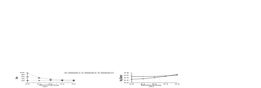
Figure 6: (a)Score of diverse set (b)Average distance of all points

Figure 6(a) shows the scores of the result set $\cal R$ for the three different datasets. With increase in MinDiv, the score of the result set decreases as expected because of the increase in the distance of points and hence their harmonic mean value. Figure 6(b) shows the average distance of the points in $\cal R$ for the three datasets. It shows the cost to be paid in terms of distance in order to obtain result diversity. The important point to note here is that in all the three datasets, for values of MinDiv up to 0.2, the distance increase is marginal. Since we expect that users will typically use MinDiv values between 0 and 0.2, it means that diversity can be obtained at relatively little cost in terms of distance.

Note that that the graphs for Dataset 3 are almost flat in both Figures 6(a) and  6(b). This is because of the high skew along each dimension in this dataset and the uniformly distributed query workload, which makes the spatially-nearest neighbors themselves to be diverse for most of the queries.

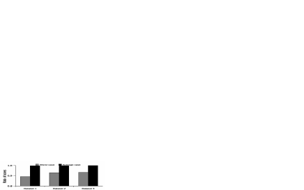
Figure 7: MOTLEY vs. Optimal

We now move on to characterizing the quality of the result set provided by Motley, which is a greedy online algorithm, against an optimal off line algorithm. This performance perspective is shown in Figure 7 which presents the average and worst case ratio of the result set scores for all three datasets. As can be seen in figure, the average case is almost optimal (note that the Y-axis of the graph begins from 0.8), indicating that Motley typically produces a close-to-optimal solution. Further, even in the worst-case, the difference is only around ten percent. We further investigated this issue by evaluating, for the cases where the Motley and optimal were different, the percentage of points that were common between the Motley result set and the optimal-set. Our experimental results showed that more than 90 percent of the answers were common. That is, even in the cases where a sub-optimal choice was made, the errors were mostly restricted to one or two points, out of the total of ten answers.

4.2 Execution Efficiency

Figure 8: (a) Average number of tuples read             (b) Percentage of sequential scan

Having established the high-quality of Motley answers, we now move on to evaluating its execution efficiency. In Figure 8(a), we show the average fraction of tuples read to produce the result set as a function of MinDiv for all three datasets. We see here that at lower values of MinDiv, the number of tuples read are small because we obtain $K$ diverse tuples after processing only a small number of points. At higher values of MinDiv, the number of MBRs pruned are more and hence tuples read are less. For example, with Dataset 2, we always read less than 14% of the total tuples.

An important point to note here is that the performance of the traditional KNN search, obtained by setting MinDiv = 0, is extremely good, indicating that Motley is a general algorithm that does not sacrifice performance on traditional KNN search in order to accommodate diversity goals. To further confirm this, we compared the performance of MOTLEY with respect to the reported performance of the Dyn KNN algorithm[6] for Datasets 1 and 2, with $K=100$. While for the small-sized Dataset 1, the number of tuples read by Dyn and MOTLEY were nearly the same, for the comparatively larger Dataset 2, the number of tuples read by Dyn was nearly 2% whereas MOTLEY reads only 0.5%.

Figure 8(b) shows the percentage of time required by Motley with respect to sequential scan for different values of MinDiv for all three datasets. From the graph, it can be seen that as data size increases Motley requires a progressively smaller percentage of time than sequential scan. Even with Dataset 1, which is a rather modest 32,561 tuples in size, Motley requires less than 40% of the time taken by sequential scan. When we consider the much larger Dataset 2, which contains more than half a million tuples, Motley consistently takes only about 10% of the sequential scan time. Further, note that the numbers reported here are conservative since the sorting of the dataset required by sequential scan was done in memory by allocating sufficient resources – in the general case, however, external sorting would have to be carried out, and the performance of sequential scan would become even worse.

To quantify the impact of pruning, we ran Motley with and without the pruning optimizations. Figure 9 shows a sample performance on Dataset 1 with K=10 and default settings. We see here that a substantial improvement is produced by the inclusion of these pruning optimizations.

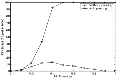
Figure 9: Impact of Pruning

4.3 Effect of K

Figure 10: Average number of tuples read for different values of K (a) Dataset 1 (b) Dataset 2 (c) Dataset 3

This experiment evaluates the effect of $K$, the number of answers, on the algorithmic performance. Figure 10 shows the percentage of tuples read as a function of MinDiv for different values of K ranging from 1 to 100. For $K=1$, it is equivalent to the traditional NN search, irrespective of MinDiv, due to requiring the closest point to form part of the result set. As the value of $K$ increases, the number of tuples read also increases, especially for higher values of MinDiv. However, we can expect that users will specify lower values of MinDiv for large $K$ settings. Dataset 1 contains only 32561 tuples so the size of the MBR represented by each R-Tree node is too large for pruning to be effective. Therefore, at $K=50$ and $K=100$, almost the entire database is scanned.

4.4 Partially-specified Point Query

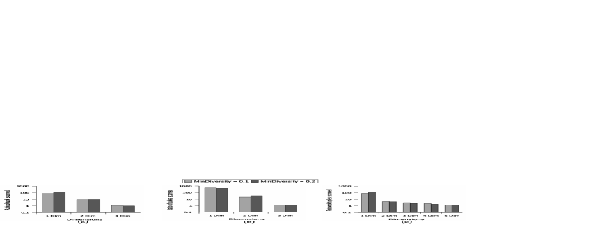
Figure 11: Ratio of tuples read for partially-specified queries (a)Dataset 1 (b)Dataset 2 (c)Dataset 3

We now move on to evaluating the performance when the point attributes in the query specify only a subset of the database dimensions. An issue here is whether we should build an R-tree specifically on the point attributes or should we simply project the global R-tree built across all dimensions onto the point attributes. Ideally, we would like to have only a single global R-tree, since building R-trees for all possible combinations of attributes ($2^{D}$) is prohibitively expensive, as mentioned earlier in Section 3. We measure the performance impact of these alternative choices here.

Figure 11 shows the ratio of tuples read for a global R-tree as opposed to a customized R-tree for all three data sets, as a function of the number of point attribute, for MinDiv settings of 0.1 and 0.2. We see here that while reduction of one or two dimensions does not unduly increase the number of tuples read, the performance degrades substantially at lower dimensions – this is because the overlap among MBRs in the global R-tree becomes high at these low dimensions.

This suggests that if the query workload has a large number of low-dimensional queries, it may be worthwhile to build a carefully chosen hierarchy of R-trees, some catering to the low dimensions and others catering to the higher dimensions.

5 Related Work

To the best of our knowledge, the KNDN problem investigated in this paper has not appeared elsewhere in the literature. It has its roots in the KNN problem, sometimes referred to as Top-K, that has been extensively studied in the last decade – we refer the reader to [6, 12] for recent surveys of this literature. The two major trends in this corpus is one based on computing nearest K using standard database statistics (e.g., [6]), while the other is based on spatial indices such as the R-tree (e.g., [12, 18]) – we have used the latter approach in this paper.

It may appear that an alternative solution to the KNDN problem would be to initially process the data into clusters using algorithms such as BIRCH [19], replace all clusters by their representatives, and then to apply the traditional KNN approach on this summary database. There are two problems here: Firstly, since the clusters are pre-determined, there is no way to dynamically specify the desired diversity, which may vary from one user to another or may be based on the specific application that is invoking the KNDN search. Secondly, since the query attributes are not known in advance, we potentially need to do clustering in each subspace of dimensions, which may become infeasible due to the exponential number of such subspaces. Finally, this approach cannot provide the traditional KNN results.

Yet another approach to produce a diverse result set could be to run the standard KNN algorithm, cluster its results, replace the clusters by their representatives, and then output these representatives as the diverse set. The problem with this approach is that it is not clear what the original number of required answers should be set to such that there are finally K representatives. If the original number is set too low, then the search process has to be restarted, whereas if the original number is set too high, a lot of wasted work ensues.

Finally, the Skyline operator [3] implements a different notion of “interesting” tuples in that, given a database of tuples, it finds the dominating tuples among this set. A tuple $T_{1}$ is said to dominate $T_{2}$ if $T_{1}$ is superior to $T_{2}$ in all attributes with respect to given query point. The skyline operator returns the set of tuples that are not dominated by any of the other tuples in the database. It is different from our approach in that the notion of domination is not with respect to a query point, and further it is possible that the results may be highly clustered spatially, resulting in very low diversity from our perspective.

6 Conclusions

In this paper, we introduced the problem of finding the K Nearest Diverse Neighbors (KNDN), where the goal is to find the closest set of answers such that the user will find each answer sufficiently different from the rest, thereby adding value to the result set. We provided a quantitative notion of diversity that ensured that two tuples were diverse if they differed in at least one dimension by a sufficient distance, and presented a two-level scoring function to integrate the orthogonal notions of distance and diversity.

We presented MOTLEY, an online algorithm for addressing the KNDN problem, based on a greedy approach integrated with a distance browsing technique. A buffered variation of Motley was introduced to improve the solution quality of the basic greedy approach, while pruning optimizations were incorporated to improve the runtime efficiency. Our experimental results with a variety of real and synthetic data-sets demonstrated that Motley can provide high-quality diverse solutions at a low cost in terms of both result distance and processing time. In fact, Motley’s performance was close to the optimal in the average case and only off by around ten percent in the worst case.

In our future work, we plan to extend our implementation of Motley to handle categorical attributes in accordance with the mechanisms discussed in this paper.

References

- [1] N. Beckmann, H. Kriegel, R. Schneider and B. Seeger, The R∗-tree: An efficient and robust access method for points and rectangles, Proc. of ACM SIGMOD Intl. Conf. on Management of Data, 1990.
- [2] S. Berchtold, D. Keim and H. Kriegel, The X-tree: An Index Structure for High-Dimensional Data, Proc. of Intl. Conf. on Very Large Data Bases, 1996.
- [3] S. Borzsonyi, D. Kossmann and K. Stocker, The Skyline Operator, Proc. of Intl. Conf. on Data Engineering, 2001.
- [4] L. Breiman, J. Friedman, R. Olshen and C. Stone, Classification and Regression Trees , Chapman and Hall, 1984.
- [5] J. Gower, A general coefficient of similarity and some of its properties, Biometrics 27, 1971.
- [6] N. Bruno, S. Chaudhuri and L. Gravano, Top-K Selection Queries over Relational Databases: Mapping Strategies and Performance Evaluation, ACM Trans. on Database Systems, 27(2), 2002.
- [7] P. Ciaccia, M. Patella and P. Zezula, M-Tree: An Efficient Access Method for Similarity Search in Metric Spaces, Proc. of Intl. Conf. on Very Large Data Bases, 1997.
- [8] V. Ganti, J. Gehrke and R. Ramakrishnan, CACTUS-Clustering Categorical Data using Summaries, Proc. of ACM Knowledge and Data Discovery Conf., 1999.
- [9] M. Grohe, Descriptive and Parameterized Complexity, Computer Science Logic, 13th Workshop, number 1683 in Lecture Notes in Computer Science, pages 14-31. Springer-Verlag, September 1999.
- [10] A. Guttman, R-trees: A dynamic index structure for spatial searching, Proc. of ACM SIGMOD Intl. Conf. on Management of Data, 1984.
- [11] A. Henrich, The LSD-tree: An Access Structure for Feature Vectors, Proc. of Intl. Conf. on Data Engineering, 1998.
- [12] G. Hjaltason and H. Samet, Distance Browsing in Spatial Databases, ACM Trans. on Database Systems, 24(2), 1999.
- [13] A. Jain, P. Sarda and J. Haritsa, Providing Diversity in K-Nearest Neighbor Query Results, Tech. Report, DSL, Indian Institute of Science, 2003.
- [14] R. Kothuri, S. Ravada and D. Abugov, Quadtree and R-tree indexes in Oracle Spatial: A comparison using GIS data, Proc. of ACM SIGMOD Intl. Conf. on Management of Data, 2002.
- [15] C. Li and G. Biswas, Conceptual Clustering with Numeric and Nominal Mixed Data – A New Similarity Based System, IEEE Trans. on Knowledge and Data Engineering, 14(4), 2002.
- [16] www.elibronquotations.com
- [17] G. Qian, Q. Zhu, Q. Xue and S. Pramanik, The ND-Tree: A Dynamic Indexing Technique for Multidimensional Non-ordered Discrete Data Spaces, Proc. of Intl. Conf. on Very Large Data Bases, 2003.
- [18] N. Roussopoulos, S. Kelley and F.Vincent, Nearest Neighbor Queries, Proc. of ACM SIGMOD Intl. Conf. on Management of Data, 1995.
- [19] T. Zhang, R. Ramakrishnan and M. Livny, BIRCH: An Efficient Data Clustering Method for Very Large Databases, Proc. of ACM SIGMOD Intl. Conf. on Management of Data, 1996.
- [20] G. Zipf. Human behaviour and the principle of least effort. Addison-Wesley, 1949.
- [21] ftp://ftp.ics.uci.edu/pub/machine-learning-databases/census-income
- [22] ftp://ftp.ics.uci.edu/pub/machine-learning-databases/covtype
- [23] http://www.cs.ucr.edu/marioh/spatialindex/