On the Continuous Fermat-Weber Problem

Abstract

We give the first exact algorithmic study of facility location problems that deal with finding a median for a continuum of demand points. In particular, we consider versions of the “continuous $k$-median (Fermat-Weber) problem” where the goal is to select one or more center points that minimize the average distance to a set of points in a demand region. In such problems, the average is computed as an integral over the relevant region, versus the usual discrete sum of distances. The resulting facility location problems are inherently geometric, requiring analysis techniques of computational geometry. We provide polynomial-time algorithms for various versions of the $L_{1}$ 1-median (Fermat-Weber) problem. We also consider the multiple-center version of the $L_{1}$ $k$-median problem, which we prove is NP-hard for large $k$.

MSC Classification: 90B85, 68U05

ACM Classification: F.2.2

Keywords: location theory, Fermat-Weber problem, $k$-median, median, continuous demand, computational geometry, geometric optimization, shortest paths, rectilinear norm, computational complexity

1 Introduction

“There are three important factors that determine the value of real estate – location, location, and location.”

The Fermat-Weber Problem.

There has been considerable study of facility location problems in the field of combinatorial optimization. In general, the input to these problems includes a weighted set $D$ of demand locations, with weight distribution $\delta$ and total weight $\mu$, a set $F$ of feasible facility locations, and a distance function $d$ that measures cost between a pair of locations. In one important class of questions, the problem is to determine one or more feasible median locations $c\in C\subseteq F$ in order to minimize the average cost from the demand locations, $p\in D$, to the corresponding central points $c_{p}\in C$ that are nearest to $p$:

$$\min_{C\subset F}\frac{1}{\mu}\int\limits_{p\in D}\delta(p)d\left(p,C\right)dp,$$

where $d(p,C)=\min_{c\in C}d(p,c)$. If there is one median point to be placed, the problem is known as the classical Fermat-Weber problem; its history reaches back to Fermat, who first posed it for three points, a case that was first solved by Torricelli. (Note that this special case has another natural generalization: in the well-known Steiner tree problem, the objective is to find a connected network of minimum total length connecting a given set of points. See [23] for a recent study of the relation between these problems and further discussion.) In the context of facility location, the median problem was discussed in Weber’s 1909 book on the pure theory of location for industries [59] (see [61] for a modern survey); because of this connection, we will speak of the Fermat-Weber problem (FWP) throughout this paper. More generally, for a given number $k\geq 1$ of facilities, the problem is known as the $k$-median problem. A problem of similar type with a different objective function is the so-called $k$-center problem, where the goal is to find a set of $k$ center locations such that the maximum distance of the demand set from the nearest center location is minimized.

Geometric Facility Location.

There is a vast literature on location theory; for a survey, see the book of Drezner [18], with its over 1200 citations that not only include papers dealing with mathematical aspects of optimization and algorithms, but also various applications and heuristics. A good overview of research with a mathematical programming perspective is given in the book of Mirchandani and Francis [45].

With many practical motivations, geometric instances of facility location problems have attracted a major portion of the research to date. In these instances, the sets $D$ of demand locations and $F$ of feasible placements are modeled as points in some geometric space, typically $\Re^{2}$, with distances measured according to the Euclidean ($L_{2}$) or Manhattan ($L_{1}$) metric. In these geometric scenarios, it is natural to consider not only finite (discrete) sets $F$ of feasible locations, but also (continuous) sets having positive area. For the classical Fermat-Weber problem, the set $F$ is the entire plane $\Re^{2}$, while $D$ is some finite set of demand points.

There has been considerable activity in the computational geometry community on facility location problems that involve computing geometric “centers” and medians of various types. The problem of determining a 1-center, i.e., a point $c$ to minimize the maximum distance from $c$ to a discrete set $D$ of points, is the familiar minimum enclosing disk problem, which has linear-time algorithms based, e.g., on the methods of Megiddo. The geodesic 1-center of simple polygons has an $O(n\log n)$ algorithm [53]; in this version of the center problem, distances are measured according to shortest paths (geodesics) within a simple polygon. Recent results of Sharir et al. [9, 22, 55] have yielded nearly-linear-time algorithms for the planar two-center problem. The more general $p$-center problem has been studied recently by [56].

Continuous Location Problems.

Location theory distinguishes between discrete and continuous location theory (see [27]). However, for median problems, this distinction has mostly been applied to the set of feasible placements, distinguishing between discrete and continuous sets $F$. It is remarkable that, so far, continuous location theory of median problems has almost entirely treated discrete demand sets $D$ [27, 52]. We should note that there are several studies in the literature that deal with $k$-center problems with continuous demand, e.g, see [43, 58], where demand arises from the continuous point sets along the edges in a graph. See [57] for results on the placement of $k$ capacitated facilities serving a continuous demand on a one-dimensional interval. Also, $k$-center problems have been studied extensively in a geometric setting, see e.g. [1, 17, 28, 30, 32, 33, 34, 35, 36, 42, 44, 55, 56]. However, designing discrete algorithms for $k$-center problems can generally be expected to be more immediate than for $k$-median problems, because the set of demand points that determine a critical center location will usually form just a finite set of $d+1$ points in $d$-dimensional space.

Continuous demand for $k$-median problems is also missing from the classification in [6]. We contend that the practical and geometric motivations of the problem make it very natural to consider exact algorithms for dealing with a continuous demand distribution for $k$-median problems: if a demand occurs at some position $p\in D$, according to some given probability density $\delta(p)$, then we may be interested in minimizing the expected distance $\int_{p\in D}d(c,p)\delta(p)dp$ for a feasible center location $c\in F$.

To the best of our knowledge, there are only few references that discuss $k$-median problems with continuous demand: See the papers [51, 65] for a discussion of continuous demand that arises probabilistically by considering a discrete demand in an unbounded environment with a large number of demand points, leading to a heuristic for optimal placement of many center points. Drezner [19] describes in Chapter 2 of his book that normally a continuous demand is replaced by a discrete one, for which the error is “quite pronounced for some problems”. (See his chapter for some discussion of the resulting error.) Wesolowsky and Love [62] (and also in their book [41] with Morris) and Drezner and Wesolowsky [20] consider the problem of continuous demand for rectilinear distances. Practical motivations include the modeling of postal districts and facility design. They compute the optimal solution for one specific example, but fail to give a general algorithm. More recently, Carrizosa, Muñoz-Márquez, and Puerto [7, 8] use convexity properties for problems of this type to deal with the error resulting from nonlinear numerical methods for approximating solutions. It should be noted that the objective function is no longer convex when distances are computed in the presence of obstacles.

In this paper, we study the $k$-median problem, and its specialization to the Fermat-Weber problem ($k=1$), in the case of continuous demand sets. Another way to state our continuous Fermat-Weber (1-median) problem is as follows: In a geometric domain (e.g., cluttered with obstacles), determine the ideal “meeting point” $c^{*}$ that minimizes the average time that it takes an individual, initially located at a random point in $D$, to reach $c^{*}$. Another application comes from the problem of locating a fire station in order to minimize the average distance to points in a neighborhood, where we consider the potential emergencies (demands) to occur at points in a continuum (the region defining the neighborhood $D$). As we noted above, this objective function is different from the situation in which we want to minimize the maximum distance instead, a problem that has been studied extensively in the context of discrete algorithms.

Choice of Metric.

Many papers on geometric location theory have dealt with continuous sets $F$ of feasible placements, including [2, 5, 13, 14, 16, 21, 37, 38, 39, 62, 63, 64]. In the majority of these papers, distances are measured according to the $L_{1}$ metric. In fact, it was shown by Bajaj [3] that if $L_{2}$ distances are used, then even in the case of only five demand locations ($|D|=5$), the problem cannot be solved using radicals; in particular, it cannot be solved by exact algorithmic methods that use only ruler and compass. (Chandrasekaran and Tamir [10] give a polynomial-time approximation scheme that uses the ellipsoid method.) In this paper, we too concentrate on the problem using the $L_{1}$ metric. While we can exactly solve some very simple special cases in the $L_{2}$ metric, in general the integrations that are required to solve the problem are likely to be just as intractable as the classic Fermat-Weber problem.

Summary of Results.

In this paper, we give the first exact algorithmic results for location problems that are continuous on both counts, in the set $D$ as well as the set $F$. In our model $D$ and $F$ are each given by polygonal domains. Our goal is to compute a set of $k$ ($k\geq 1$) optimal centers in the feasible set $F$ that minimize the average distance from a demand point of $D$ to the nearest center point. Our results include:

(1)

A linear-time ($O(n)$) algorithm for computing an optimal solution to the 1-median (Fermat-Weber) problem when $D=F=P$, a simple polygon having $n$ vertices, and distance is taken to be $L_{1}$ geodesic distance inside $P$.

(2)

An $O(n^{2})$ algorithm for computing an optimal 1-median for the case that $D=F=P$, a polygon with holes, and distance is taken to be (straight-line) $L_{1}$ distance.

(3)

An $O(I+n\log n)$ algorithm (where $I=O(n^{4})$ is the complexity of a certain arrangement) for computing an optimal 1-median for the case that $D=F=P$, a polygon with holes, and distance is taken to be $L_{1}$ geodesic distance inside $P$.

(4)

A proof of NP-hardness for the $k$-median problem when the number of centers, $k$, is part of the input, and $D=F=P$ is a polygon with holes. This adds specific meaning to the statement by Wesolowsky and Love [62] that computing the optimal position of several locations “is obviously very tedious when (the number of locations) is very large”.

(5)

Generalizations of our results to the following cases: non-uniform probability densities over the demand set $D$; fixed-orientation metrics (generalization of $L_{1}$), which can be used to approximate the Euclidean metric; higher dimensions; and, $F\neq D$ for straight-line distances.

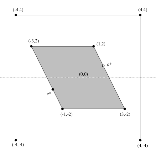
Figure 1: A simple example in which the region $D=F=P$ is a polygon (square) with a single (parallelogram) hole, shown shaded. The average straight-line $L_{1}$ distance is minimized by two optimal center points, each marked “$c^{*}$”, on the boundary of $P$. This example is analyzed in more detail later; refer to Figure 10.)

This paper represents research done as part of the PhD thesis of Weinbrecht; additional examples, discussion, and details may be found in [60].

2 Preliminaries

Basic Definitions.

We will let $Z=(x,y)$ denote a candidate center point in $F\subseteq\Re^{2}$. (We concentrate on two-dimensional problems until Section 8, where we discuss extensions to higher dimensions.) We defer discussion of multiple center points ($k>1$) to Section 7; for now, $k=1$ and we consider the Fermat-Weber (1-median) problem.

We let $P$ denote a polygonal domain: This is a connected planar set of points that is bounded by a finite set of disjoint simple closed polygonal curves. We assume that $P$ is nondegenerate, i.e., it is a closed set that equals the closure of its interior points; in particular, the interior is connected. We say that the vertices of $P$ are the vertices of its boundary; as part of the nondegeneracy assumption, we assume that each vertex is incident to precisely one boundary polygon and to two edges. In the case of one connected boundary, we say that a polygon $P$ is simple; otherwise we say that $P$ has one or several holes, i.e, bounded components of the complement $\Re^{2}\setminus P$. A critical vertex $v$ of $P$ is one that has locally extremal $x$- or $y$-coordinate relative to the boundary component containing $v$, and an interior angle of at least $\pi$. A chord of $P$ is a straight line segment within $P$ that connects two points on the boundary of $P$. If $P$ is a simple polygon, any chord subdivides $P$ into two or more pieces.

For purposes of our discussions, we focus on the case in which $D=F=P$: we restrict $Z$ to $P$, which also equals the demand set. Furthermore, we focus our discussion to the case in which the demand is uniformly distributed over the set $D=P$, so our goal is to minimize the average distance, $f(Z)$, given by the integral

$$f(Z)=f(x,y)=\frac{1}{\mu}{\int\!\int}_{(u,v)\in P}d(Z,(u,v))dudv,$$

where $\mu$ is the total area of $P$, $d(\cdot,\cdot)$ denotes either (straight-line) $L_{1}$ distance or geodesic (shortest-path) $L_{1}$ distance within $P$. (We abuse notation slightly by writing $f(Z)=f((x,y))=f(x,y)$.)

Shortest Path Maps.

In order to analyze the $k$-median problem with respect to geodesic distances, we will utilize several definitions and results from the theory of geometric shortest paths among obstacles; see Mitchell [49, 50] for surveys on the subject of geometric shortest paths.

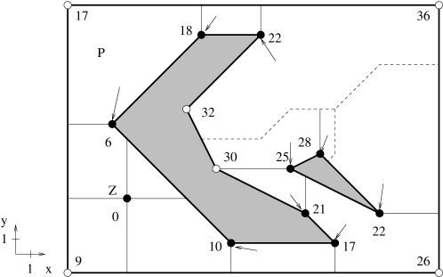
Figure 2: An example of the $L_{1}$ geodesic SPM($Z$) for a polygon $P$ with two holes (shaded). Vertices are labeled with their $L_{1}$ geodesic distances from $Z$. The cell rooted at $Z$ is partitioned into four quadrants by a vertical and a horizontal chord through $Z$. Within each other cell, rooted at a vertex of $P$, an arrow is drawn pointing to the root of the cell. Vertices of $P$ whose cells are nonempty are drawn as solid black dots; the white vertices have empty cells in SPM($Z$).

For a given geometric environment $P$, the shortest-path map, SPM($Z$) with respect to source point $Z$ represents the set of shortest paths within $P$ from $Z$ to all other points $t\in P$. The SPM($Z$) is a decomposition of $P$ into cells $\sigma$, each having a unique root vertex, $r_{\sigma}$, such that a shortest path within $P$ from $Z$ to $t\in P$ is given by following a shortest path within $P$ from $Z$ to $r_{\sigma}$, then going from $r_{\sigma}$ to $t$ directly along a “straight” segment. A straight segment between $p\in P$ and $q\in P$ is a path whose length is $d(p,q)$, where $d(\cdot,\cdot)$ denotes our underlying distance function ($L_{1}$, $L_{2}$, etc.). If the underlying distance is $L_{2}$, a straight segment is necessarily a straight line segment; if the underlying distance is $L_{1}$, as in most of this paper, a straight segment from $p$ to $q$ consists of any path from $p$ to $q$ that is both $x$-monotone and $y$-monotone (e.g., an “L-shaped” path or a “staircase” is straight in the $L_{1}$ metric). If $t$ lies in a cell $\sigma$ rooted at $r_{\sigma}$, the geodesic distance from $Z$ to $t$ is given by $d_{G}(Z,t)=d_{G}(Z,r_{\sigma})+d(r_{\sigma},t)$, where $d_{G}(\cdot,\cdot)$ denotes the shortest-path (geodesic) distance function induced by $P$. There is also a cell with root $Z$, consisting of points $t\in P$ for which a shortest path from $Z$ to $t$ is attained by a straight segment $Zt$. Points $t$ on the common boundary of two or more cells are optimally reached by shortest paths to $t$ whose last segment joins $t$ to the root vertex of any one of the cells having $t$ on its boundary. Refer to Figure 2 for an example of SPM($Z$) in the $L_{1}$ geodesic metric. Each vertex $v$ of $P$ is the root of a (possibly empty) cell. A vertex $v=r_{\sigma}$ that is the root of a cell $\sigma$ lies on the boundary of a neighboring cell $\sigma^{\prime}$, so there is a shortest path from $Z$ to $r_{\sigma}$ whose last segment is $r_{\sigma^{\prime}}r_{\sigma}$; we say that $r_{\sigma^{\prime}}$ is the predecessor of $r_{\sigma}$. In addition to its predecessor, we store with each vertex $v$ of $P$ the length, $d_{G}(Z,v)$, of a shortest path within $P$ from $Z$ to $v$. In summary, SPM($Z$) is a decomposition of $P$ into cells according to the “combinatorial structure” (sequence of obstacle vertices along the path) of shortest paths from $Z$ to points in the cells.

For any two distinct vertices $u$ and $v$ of $P$, the bisector with respect to $u$ and $v$ is the locus of points $p\in P$ that are (geodesically) equidistant from $Z$ via the two distinct roots, $u$ and $v$; thus, a bisector is the (possibly empty) locus of points $p\in P$ satisfying $d_{G}(Z,p)=d_{G}(Z,u)+d(u,p)=d_{G}(Z,v)+d(v,p)$. If the underlying metric is Euclidean, bisectors are curves, easily seen to be straight line segments or hyperbolic arcs. In the $L_{1}$ geodesic metric, bisectors may be horizontal line segments, vertical line segments, polygonal chains of segments that are horizontal, vertical, or diagonal (with slope $\pm 1$), or they may, in a degenerate situation, consist of regions. See Figure 3 and Figure 4. In order that cells of the SPM($Z$) do not overlap in regions of nonzero area, and so that the SPM($Z$) is a planar decomposition of $P$, it is convenient to resolve degeneracies so that all bisectors are one-dimensional (polygonal) curves, not regions. We do this as follows. First, if $p\in P$ satisfies $d_{G}(Z,p)=d_{G}(Z,u)+d(u,p)=d_{G}(Z,v)+d(v,p)$, then we consider $p$ to be in the cell rooted at $u$ (and not in the cell rooted at $v$) if $d(u,p)<d(v,p)$; a consequence is that the points $p\in P$ that are in the cell rooted at $u$ are visible to $u$ (i.e., the segment $up$ lies in the cell). Figure 4 shows the result of applying this rule to two situations in which the $L_{1}$ geodesic bisector would otherwise be a region. Second, we infinitesimally perturb the vertices of $P$ so that no two vertices lie on a common line of slope $\pm 1$; this implies that set of points $p\in P$ for which $d_{G}(Z,p)=d_{G}(Z,u)+d(u,p)=d_{G}(Z,v)+d(v,p)$ and $d(u,p)=d(v,p)$ is a polygonal chain, not a region of nonzero area. (All of our results apply also to the unperturbed problem instances, by standard arguments.)

It is easily seen that a small horizontal (or vertical) shift of $Z$ by an amount $h$ results in a shift of the bisector between two vertices $u$ and $v$ by an amount $h/2$.

Figure 3: Examples of the $L_{1}$ bisectors between two points, $P_{1}$ and $P_{2}$, in the $L_{1}$ metric. In each of the three cases, the locus is shown of points $p$ for which $d(P_{1},p)=d(P_{2},p)$. Note that in case (c), when $P_{1}$ and $P_{2}$ lie on a line of slope $\pm 1$, the bisector includes two regions (shown shaded).

Figure 4: Examples of $L_{1}$ geodesic bisectors. In both cases, the points in the lightly shaded quadrant are equidistant from $Z$ via $u$ and via $v$; our tie-breaking rule, however, assigns the shaded bisector points to the cell rooted at $u$, resulting in the bisector curve shown dashed.

Some bisector curves, such as those horizontal and vertical segments shown solid in Figure 2, may be crossed by shortest paths from $Z$ to points $p\in P$. However, bisector curves that consist of points that are the endpoints of maximal shortest (geodesic) paths are not crossed by any shortest path; these are shown dashed in Figure 2 and are called watersheds. (A shortest path from $Z$ to $p\in P$ is maximal if it is not the proper subset of a shortest path from $Z$ to some other point $p^{\prime}\neq p$ of $P$.) One can think of the watershed bisectors as “ridges” that partition $P$ into regions according to the topological type (homotopy class) of shortest paths; a point on a watershed can be reached from at least two homotopically distinct shortest paths from $Z$.

Shortest path maps can be computed in optimal time $O(n\log n)$ for a polygon with $n$ vertices, both in the Euclidean metric and in the $L_{1}$ metric [29, 46, 48]. More generally, shortest-path maps can be applied to weighted region metrics, where the time for traveling depends on a local density function. For more information, see the surveys of Mitchell [49, 50].

Finally, we define one other piece of notation. For any position $Z$ of a center, we define two subsets of the domain $P$: the set $W(Z)$ (resp., $E(Z)$) of all points $p\in P$ for which every shortest path from $Z$ to $p$ enters the open halfplane to the left (resp., right) of $Z$ prior to entering the open halfplane to the right (resp., left) of $Z$. In other words, $W(Z)$ (resp., $E(Z)$) corresponds to the set of points $p\in P$ for which an optimal path to $p$ initially heads to the west (resp., east). Similarly, $P$ is subdivided into the sets $N(Z)$ and $S(Z)$ of points for which shortest paths initially head north versus south. These definitions apply both to geodesic distances, $d_{G}(\cdot,\cdot)$, and to straight-line distances; refer to Figure 6 for illustrations. While there may be points $p\in P$ that are not in $W(Z)\cup E(Z)$, such points either lie on the vertical line through $Z$ or, in the case of geodesic distances, lie on a bisector (since such points are reached by at least two distinct optimal paths – one heading initially east, one heading initially west). By the convention and perturbation assumption that allows us to assume that bisectors are one-dimensional curves (rather than regions), we see that $W(Z)\cup E(Z)$ covers all of $P$ except for a set of zero area; a similar statement holds for $N(Z)\cup S(Z)$. In the following, we will use $w(Z)$, $e(Z)$, $n(Z)$, $s(Z)$ for the area of $W(Z)$, $E(Z)$, $N(Z)$, $S(Z)$, respectively.

3 Local Optimality Conditions

For any given center location $Z$, the objective function value $f(Z)$ that gives the average distance from $Z$ to points of $P$ can be evaluated by decomposing $P$ into a set of “elementary” pieces, computing the average distance for each piece, and then obtaining the total average distance as a weighted sum of the average distances for the pieces. In the case of straight-line $L_{1}$ distance, we simply use a trapezoidization (or triangulation) of $P$ to determine the pieces; this can be done in linear time if $P$ is simple, or in $O(n\log n)$ time if $P$ has holes. In the case of geodesic distance, the shortest-path map, SPM($Z$), gives a decomposition of $P$ into cells (each of which can be refined into triangles or trapezoids to yield a decomposition into $O(1)$-size pieces), each having a corresponding root vertex on its boundary. By computing the average distance from points of a cell to the cell’s root $r$ and adding this average to the distance $d_{G}(Z,r)$, and then summing over all cells, we obtain the average geodesic distance, $f(Z)$.

The average distance associated with a single elementary piece is given by the following result, which can be verified easily by straightforward integration. As any region can be subdivided into a limited number of triangles of this type, it can be used as a stepping stone for computing the objective value for more complicated regions.

Figure 5: Lemma 1 notation used in computing the average $L_{1}$ distance of $\triangle ABC$ from the point $A$.

Lemma 1

For a triangle $\tau$ with vertices $A$, $B$, and $C$, such that edge $\overline{AB}$ is horizontal, let $a$ be the length of $\overline{AB}$, let $c$ be the length of the altitude from $C$, and let $b$ be the distance from $A$ to the foot of the altitude from $C$. Then the average $L_{1}$ distance of points in $\tau$ from vertex $A$ is $\frac{1}{3}(a+b+c)$.

The objective function, $f(Z)$, is a continuous function of the location of the center $Z$. Because the set $F=P$ of feasible placements is a compact domain, it follows that there is an optimum. If $Z$ is a point minimizing $f(Z)$, then, $Z$ must be locally optimal, meaning that there cannot be a feasible direction $H=(x_{H},y_{H})$, i. e., $Z+\varepsilon H\in P$ for sufficiently small $\varepsilon$, such that $f(Z)>f(Z+\varepsilon H)$. If $f$ is differentiable at some point $Z\in P$, then $\langle\nabla f(Z),H\rangle\geq 0$. In particular, for interior points that are locally optimal, the gradient must be zero; for points in the interior of boundary edges, the gradient must be orthogonal to the boundary. In the following lemma we compute the gradient of $f$:

Lemma 2

Consider the objective function $f$ for average straight-line $L_{1}$ distance in a region $P$ of area $\mu=\mu(P)$. Let $Z=(x,y)$ be a point in $P$. Then the first partial derivatives of $f$ are well-defined and given by:

$$\begin{array}[]{rcl}f_{x}(Z)&=&\frac{1}{\mu}\left(w(Z)-e(Z)\right),\\ f_{y}(Z)&=&\frac{1}{\mu}\left(s(Z)-n(Z)\right).\end{array}$$ (1)

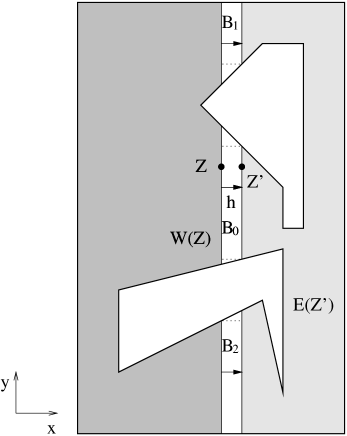
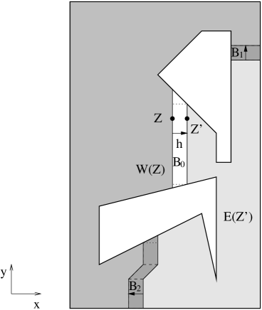
Figure 6: Computing the partial derivative $f_{x}$ for straight-line $L_{1}$ distances (on the left) and for geodesic $L_{1}$ distances (on the right).

Proof. We compute $f_{x}$; $f_{y}$ is computed similarly. Refer to Figure 6 (left). Consider the point $Z^{\prime}=Z+(h,0)$ for some sufficiently small $h$. Let $C(Z,Z^{\prime}):=\{p=(x_{p},y_{p})\in P|x\leq x_{p}\leq x+h\}$ be the narrow vertical strip between $Z$ and $Z^{\prime}$. We compute:

$$f_{x}(x,y)=\lim_{h\rightarrow 0}\frac{f(x+h,y)-f(x,y)}{h}=\lim_{h\rightarrow 0}\frac{f(Z^{\prime})-f(Z)}{h}$$

$$= \lim_{h\rightarrow 0}\left(\frac{\frac{1}{\mu}\left(\int\limits_{p\in P}d\left(p,Z^{\prime}\right)dp-\int\limits_{p\in P}d\left(p,Z\right)dp\right)}{h}\right)$$

$$= \lim_{h\rightarrow 0}\left(\frac{\frac{1}{\mu}\left(\int\limits_{p\in W(Z)}d\left(p,Z^{\prime}\right)dp-\int\limits_{p\in W(Z)}d\left(p,Z\right)dp\right)}{h}\right)$$

$$+ \lim_{h\rightarrow 0}\left(\frac{\frac{1}{\mu}\left(\int\limits_{p\in C(Z,Z^{\prime})}d\left(p,Z^{\prime}\right)dp-\int\limits_{p\in C(Z,Z^{\prime})}d\left(p,Z\right)dp\right)}{h}\right)$$

$$+ \lim_{h\rightarrow 0}\left(\frac{\frac{1}{\mu}\int\limits_{p\in E(Z^{\prime})}d\left(p,Z^{\prime}\right)dp-\int\limits_{p\in E(Z^{\prime})}d\left(p,Z\right)dp}{h}\right).$$

For small enough $h$, the area of $C(Z,Z^{\prime})$ is a linear function of $h$, since the boundary of $P$ is made up of straight line segments. The term involving the difference of the two integrals over the points $p\in C(Z,Z^{\prime})$ is dependent only on the $x$-contribution to the $L_{1}$ distance ($|x_{p}-x_{Z}|$ or $|x_{p}-x_{Z^{\prime}}|$) between $p$ and $Z$ or $Z^{\prime}$, since the $y$-contributions cancel ($y_{Z}=y_{Z^{\prime}}$). Since $x_{p}$ varies within a range of $h$, and $|x_{p}-x_{Z}|\leq h$ (and $|x_{p}-x_{Z^{\prime}}|\leq h$) as well, we get that

$$\left(\int\limits_{p\in C(Z,Z^{\prime})}d\left(p,Z^{\prime}\right)dp-\int\limits_{p\in C(Z,Z^{\prime})}d\left(p,Z\right)dp\right)\in O(h^{2}).$$

Since

$$\int\limits_{p\in W(Z)}d\left(p,Z^{\prime}\right)dp=\int\limits_{p\in W(Z)}\left(h+d\left(p,Z\right)\right)dp,$$

and

$$\int\limits_{p\in E(Z)}d\left(p,Z\right)dp=\int\limits_{p\in E(Z)}\left(h+d\left(p,Z^{\prime}\right)\right)dp,$$

we get

$$f_{x}(x_{z},y_{z})=\lim_{h\rightarrow 0}\left(\frac{\int\limits_{p\in W(Z)}h\leavevmode\nobreak\ dp-\int\limits_{p\in E(Z)}h\leavevmode\nobreak\ dp+O(h^{2})}{\mu h}\right)=\left(\frac{1}{\mu}w(Z)-e(Z)\right),$$

as claimed. $\Box$

The above lemma characterizes the gradients in the case of straight-line distances. For geodesic distances, we proceed in a similar manner; refer to Figure 6 (right). Note that the shape of $C(Z,Z^{\prime})$ is different in the case of geodesic distances. For the example in the figure, $C(Z,Z^{\prime})$ is the union of one connected strip (shown white), bounded by vertical line segments through $Z$ and $Z^{\prime}$ and the boundary of $P$, and possibly several narrow regions that are swept by the watersheds as $Z$ moves to $Z^{\prime}$ (shown darkly shaded in the figure); note that these latter regions only occur in the case of $P$ being a polygon with holes.

In the lemma below, we state the result under a technical assumption, which avoids difficulties with the continuity of $w(Z)$ and $e(Z)$, as well as with degenerate bisectors.

Lemma 3

Consider the objective function $f$ for average geodesic $L_{1}$ distance in a region $P$ of area $\mu$. Let $Z=(x_{Z},y_{Z})$ be a point in $P$; assume that neither $x_{Z}$ nor $y_{Z}$ coincide with the $x$- or $y$-coordinate of a critical vertex of $P$, and that $Z$ does not lie on a watershed bisector in a shortest path map, SPM($v$), with respect to a vertex $v$ of $P$. Then the first partial derivatives of $f$ are well-defined and given by:

$$\begin{array}[]{rcl}f_{x}(Z)&=&\frac{1}{\mu}\left(w(Z)-e(Z)\right),\\ f_{y}(Z)&=&\frac{1}{\mu}\left(s(Z)-n(Z)\right).\end{array}$$ (2)

Proof. The argument is directly analogous to the proof of Lemma 2. The assumption that $Z$ does not lie on a watershed bisector of SPM($v$) for any vertex $v$ implies that no watershed bisector of SPM($Z$) contains a vertex $v$ of $P$. This implies that the area of $C(Z,Z^{\prime})$ is a linear function of the perturbation parameter $h$. Furthermore, the difference $d(p,Z)-d(p,Z^{\prime})$ for points $p\in C(Z,Z^{\prime})$ is bounded by $h$. The claim follows, as in the previous lemma. $\Box$

In some situations, we make use of properties of higher-order derivatives of $f$. In particular, we use the following lemma:

Lemma 4

The objective function $f$ is piecewise the sum of two cubic functions, $f_{1}(x)$ and $f_{2}(y)$, both for straight-line and for geodesic distances.

Proof. We start by considering the objective function $f$ for average straight-line $L_{1}$ distances in $P$. Let $Z=(x_{Z},y_{Z})$ be a point in $P$, with neither $x_{Z}$ nor $y_{Z}$ coinciding with the $x$- or $y$-coordinate of a critical vertex of $P$. Consider a small change in the $x$-coordinate of $Z$: let $Z^{\prime}=Z+(h,0)$. Then $W(Z^{\prime})=W(Z)\cup C(Z,Z^{\prime})$ and $E(Z^{\prime})=E(Z)\cup C(Z,Z^{\prime})$, where $C(Z,Z^{\prime})=B_{0}\cup B_{1}\cup\dots\cup B_{k}$ is a union of a set of trapezoids $B_{i}$, each of width $h$; refer to Figure 6. Since the area of each trapezoid $B_{i}$ is a quadratic function of the width $h$, for small enough $h$, we get that $w(Z^{\prime})-w(Z)$ and $e(Z^{\prime})-e(Z)$ are also quadratic in $h$. Since $f_{x}(Z)=\frac{1}{\mu}(w(Z)-e(Z))$, by Lemma 3, this implies that $f_{xxx}(Z)$ is a constant. (Specifically, $f_{xxx}(Z)=(2/\mu)\sum_{i}(m_{i,t}-m_{i,b})$, where $m_{i,t}$ (resp., $m_{i,b}$) is the slope of the edge of $P$ bounding the top (resp., bottom) of trapezoid $B_{i}$.) To see that $f$ does not contain any terms that have $xy$ as a factor, note that for fixed $x$, $W(Z)$ and $E(Z)$, and thus $f_{x}(Z)$ does not depend on $y$.

For geodesic distances, the claim follows in a similar manner. Now, the regions $B_{i}$ forming the connected components of $C(Z,Z^{\prime})$ are not necessarily vertical-walled trapezoids, but have parallel walls formed by translates of watershed bisectors. See Figure 6. Instead of being trapezoids bounded by vertical chords through $Z$ and $Z^{\prime}$, however, the areas $B_{i}$ are bounded by two bisectors, corresponding to translates of watershed bisectors for $Z$ and $Z^{\prime}$. Specifically, it follows from properties of $L_{1}$ bisectors described in Section 2 that these bisectors move in a parallel fashion, provided that no degeneracy of a bisector occurs during the move from $Z$ to $Z^{\prime}$, i.e., no polygon vertex is hit by a bisector. The area of region $B_{i}$ is thus quadratic in $h$, and the result follows. Again, for fixed $x$, $f_{x}(Z)$ does not depend on $y$. $\Box$

4 Straight-Line $L_{1}$ Distance

For straight-line distances, a finite average is guaranteed even for disconnected regions $P$, as long as they are compact. In the following, we will consider local optimality for finding a global optimum of $f$. Lemma 2 motivates considering the $L_{1}$ origin of $P$, which is a point $Z$ with $w(Z)=e(Z)$ and $n(Z)=s(Z)$, i.e., the (unique) point that is both a median of the $x$- and the $y$-distribution. However, the example in Figure 7 shows that even for the special case of a simple polygon $P$, the $L_{1}$ origin of $P$ may not be a feasible point.

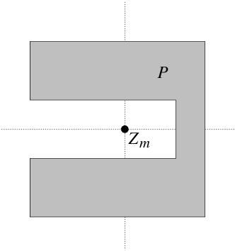
Figure 7: For straight-line distances, the $L_{1}$ origin of a simple polygon $P$ may be infeasible.

This makes it slightly involved to compute all local optima. In the following, we describe how to evaluate them in $O(n^{2})$ time.

Theorem 5

For straight-line $L_{1}$ distances, a point $Z^{*}=(x^{*},y^{*})$ in a polygonal region $P$ that minimizes the average distance $f$ to all points in $P$ can be found in time $O(n^{2})$.

Proof. We apply the local optimality conditions. We start by computing in time $O(n\log n)$ the $L_{1}$ origin $Z_{m}$ of $P$; if $Z_{m}$ is feasible (i.e., $Z_{m}\in P$), we are done. If no interior point of $P$ is a local optimum, then we have to consider the boundary of $P$. This yields a set $E$ of $O(n)$ line segments and a set $V$ of $O(n)$ vertices that we examine for local optimality.

We overlay the set of vertical and horizontal lines through all vertices of $P$ with $E$, subdividing each segment in $E$ into $O(n)$ pieces, bounded by a total of $O(n^{2})$ “overlay” vertices $V_{o}$. Let $E_{o}$ be the resulting set of $O(n^{2})$ subsegments. See Figure 8.

Figure 8: Subdivision of the polygon into cells.

Now we can examine the interior points $p_{t}=(t,y(t))$ of each edge $e_{j}\in E_{o}$ for local optimality. Let $s_{j}$ be a vector parallel to $e_{j}$. By construction of $E_{o}$, the vertical and horizontal lines through $p_{t}$ cannot encounter a vertex of $P$ as $p_{t}$ slides along one subsegment of $E_{o}$. Thus, it follows from Lemma 4 that $f_{x}(p_{t})$ is a quadratic function in $t$, and so is $f_{y}(p_{t})$. Therefore, considering for $Z\in e_{j}$ the local optimality condition

$$\langle\nabla f(p_{t}),s_{j}\rangle=0$$

for all $O(n^{2})$ subsegments $e_{j}\in E_{o}$ yields a set of $O(n^{2})$ quadratic equations in $t$. These can be solved in amortized time $O(n^{2})$, because we can obtain the coefficients of each quadratic equation in amortized constant time by advancing from cell to cell in the overlay arrangement. This gives, for each subsegment $e_{j}$, at most two local optima, $q_{j,1}$ and $q_{j,2}$. Let $V_{\ell}$ be the union of $E_{o}$ and all $q_{j,1}$ and $q_{j,2}$. By construction, $V_{\ell}$ contains $O(n^{2})$ elements, and all local optima of $f$ occur at points of $V_{\ell}$. Thus, our goal is to evaluate the objective function at each of these points and to select the best one. This is simply done in amortized time $O(1)$ per candidate, by walking over the overlay arrangement and incrementally updating the value of the objective function. $\Box$

In many cases, the following property of straight-line medians can be applied for a reduction of the set of boundary segments that we need to consider. (See Figure 9 for an illustration.) If $Z_{m}=(x_{m},y_{m})$ is the $L_{1}$ origin of $P$ and $p_{1}=(x_{1},y_{1})$ and $p_{2}=(x_{2},y_{2})$ are points in $P$, we say that $p_{1}$ dominates $p_{2}$, if $p_{1}$ lies in the rectangle spanned by $Z_{m}$ and $p_{2}$.

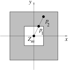
Figure 9: In the region $P$ (shown shaded), $p_{2}$ is dominated by $p_{1}$ and cannot be a local optimum.

Lemma 6

Let $p_{1}=(x_{1},y_{1})$ and $p_{2}=(x_{2},y_{2})$ be points in $P$. If $p_{1}$ dominates $p_{2}$, then $f(p_{1})\leq f(p_{2})$.

Proof. Suppose that $x_{2}>x_{1}\geq x_{m}$ and $y_{2}\geq y_{1}\geq y_{m}$. Then $w(p_{2})\geq w(p_{1})\geq\frac{\mu}{2}$ and $s(p_{2})\geq s(p_{1})\geq\frac{\mu}{2}$, so moving a center from $p_{2}$ to $p_{1}$ cannot increase the objective value. $\Box$

Using a plane-sweep algorithm, it is possible to identify the non-dominated portions of the boundary in time $O(n\log n)$. If this set has complexity $o(n)$, then we get a reduction of the overall complexity.

A simple example of the problem solved in this section is shown in Figure 10 (based on the example given in Figure 1). This example shows the necessity of solving quadratic equations in computing the optimal solutions (points $p_{4}$ and $p_{5}$). The non-dominated points are $p_{1}$, $p_{2}$, and $p_{3}$, as well as the points interior to the segment $e_{2,3}=\overline{p_{2}p_{3}}$.

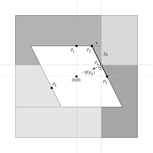
Figure 10: The example from Figure 1 is analyzed for the case of straight-line $L_{1}$ distances. There are two optimal center points: $p_{4}=(2\sqrt{7}-\frac{9}{2},11-4\sqrt{7})$ and its mirror image, $p_{5}$.

5 Geodesic $L_{1}$ Distances in Simple Polygons

In this section, we show how to compute in optimal ($O(n)$) time a point that minimizes the average geodesic $L_{1}$ distance for a simple polygon $P$ without holes.

From Lemma 3, we know that the partial derivative $f_{x}(Z)=\frac{1}{\mu}(w(Z)-e(Z))$ vanishes if $w(Z)=e(Z)$. Therefore we consider the functions $w(Z)$ and $e(Z)$ that are well-defined even for points for which the gradient is not. As $x$ increases, $w(Z)$ increases monotonically, while $e(Z)$ decreases monotonically. Note that $w(Z)$ may be discontinuous at critical vertices of $P$: As shown in Figure 13, an entire region may switch from “east” to “west” as a vertical chord passes through a critical vertex.

However, even discontinuous behavior at critical coordinates does not impair monotonicity of $w(Z)$ and $e(Z)$, so there is still a well-defined vertical median chord $c_{x}$ at some $x$-coordinate $x_{m}$ such that $w(Z_{1})<e(Z_{1})$ for all $Z_{1}=(x_{1},y_{1})$ with $x_{1}<x_{m}$ (implying $f_{x}(Z_{1})<0$ just left of $x_{m}$), and $w(Z_{1})>e(Z_{1})$ for all $Z_{2}=(x_{2},y_{2})$ with $x_{2}>x_{m}$ (implying $f_{x}(Z_{2})>0$ just right of $x_{m}$). Similarly, there is a unique horizontal median chord $c_{y}$ at $y$-coordinate $y_{m}$. Again we call $Z_{m}=(x_{m},y_{m})$ the $L_{1}$ origin of $P$.

In the following, we use the structure of simple polygons to show that the locally optimal point $Z_{m}$ has to belong to the feasible region $P$ (possibly on the boundary of $P$), implying that it is a unique global optimum.

Theorem 7

The point $Z_{m}$ is feasible (lies in $P$) and thus a unique global optimum, minimizing the average $L_{1}$ geodesic distance to points in $P$.

Proof. The chord $c_{x}$ subdivides $P$ into two pieces: let $E$ denote the part to the right (“east”) of $c_{x}$, and $W$ the part to the left (“west”) of $c_{x}$. Note that $E$ or $W$ may consist of two or more connected components only if $c_{x}$ passes through a critical vertex. Similarly, the chord $c_{y}$ subdivides $P$ into the region $N$ (“north”) that lies above $c_{y}$, and the region $S$ (“south”) that lies below $c_{y}$.

We claim that $c_{x}$ and $c_{y}$ intersect at a point ($Z_{m}$) inside $P$. The proof is by contradiction; assume that $Z_{m}$ lies outside $P$. We will distinguish the following cases.

Case 0: Neither $c_{x}$ nor $c_{y}$ are critical. If $Z_{m}\not\in P$, then simplicity of $P$ implies that the two chords subdivide $P$ into three pieces; this means that precisely one of the pieces $W$ and $E$ has nonempty intersection with one of the pieces $N$ and $S$. Without loss of generality, assume that the two chords subdivide $P$ into the three pieces, $E$, $N\cap W$, and $S$, as shown in Figure 11. Since $P$ is a nondegenerate polygon, the corresponding areas, $\mu(E)$, $\mu(N\cap W)$, and $\mu(S)$, are all positive, with $\mu(E)+\mu(S)+\mu(N\cap W)=\mu(P)=\mu$. However, the local optimality of $x_{m}$ implies that $\mu(E)=\frac{\mu}{2}$ and the local optimality of $y_{m}$ implies that $\mu(S)=\frac{\mu}{2}$, implying the contradiction that $\mu(N\cap W)=0$.

Figure 11: Case 0: Neither of the median chords $c_{x}$ and $c_{y}$ is critical.

Case 1: Exactly one of $c_{x}$ and $c_{y}$ is critical. Without loss of generality, assume that $c_{y}$ passes through a critical vertex of $P$ that is a local maximum of the boundary of $P$, as in Figure 12. As in Case 0, the (noncritical) vertical chord $c_{x}$ partitions $P$ into two pieces, $E$ and $W$, each of area $\frac{\mu}{2}$. Also, $c_{y}$ partitions $P$ into one “upper” piece $N$ and two “lower” pieces, $S_{1}$ and $S_{2}$, each with positive area. (In degenerate situations, $c_{y}$ may pass through multiple critical vertices, resulting in multiple lower pieces; our arguments includes this case by considering additional pieces as part of $S_{2}$.) The assumption that $c_{x}$ and $c_{y}$ do not cross inside $P$ implies that either $W$ or $E$ is a strict subset of $S_{1}$, $S_{2}$, or $N$. This is a contradiction, since $\mu(W)=\mu(E)=\frac{\mu}{2}$, and $\mu(N)=\frac{\mu}{2}$, $\mu(S_{1})<\frac{\mu}{2}$, and $\mu(S_{2})<\frac{\mu}{2}$.

Figure 12: Case 1: Exactly one of the median chords is critical.

Case 2: Both $c_{x}$ and $c_{y}$ are critical. Without loss of generality, assume that $c_{x}$ passes through a critical vertex of $P$ that is a local minimum of the boundary, while $c_{y}$ passes through a critical vertex that is a local maximum of the boundary, as shown in Figure 13. As in Case 1, the horizontal chord $c_{y}$ subdivides $P$ into a “northern” piece $N$, and two “southern” pieces, $S_{1}$ and $S_{2}$, each with positive area. Similarly, the vertical chord $c_{x}$ subdivides $P$ into a “western” piece $W$, and two “eastern” pieces, $E_{1}$ and $E_{1}$, each with positive area. We assume further, without loss of generality, that the critical vertex through which $c_{x}$ passes lies within the piece $S_{1}$, as shown in the figure. We have a contradiction in the fact that $\mu(N)=\mu(W)=\frac{\mu}{2}$, while the set $P\setminus(N\cup W)$ has positive area greater than $\mu(S_{2})$. $\Box$

Figure 13: Case 2: Both of the median chords are critical.

Theorem 8

The point $Z_{m}$ can be computed in linear time.

Proof. We describe how to compute the $x$-coordinate $x_{m}$ of $Z_{m}$; the $y$-coordinate is found in a similar manner.

In linear time (using Chazelle’s algorithm [11]), we build the vertical trapezoidization of $P$, which is defined by drawing vertical chords through every vertex of $P$. Each piece, $\tau_{i}$, of the resulting subdivision is either a vertical-walled trapezoid or a triangle having one side vertical (such a triangle can be considered to be a degenerate vertical-walled trapezoid). Consider the adjacency graph ${\cal G}$ of these pieces $\tau_{i}$ (i.e., the planar dual of the trapezoidization); because $P$ is a simple polygon, ${\cal G}$ is a tree.

Figure 14: A median trapezoid corresponds to a median in a node-weighted tree, with node weight representing trapezoid area.

Let $\tau_{m}$ denote the trapezoid containing the vertical chord $c_{x}$ through $Z_{m}$. (We assume, without loss of generality, that $c_{x}$ is not one of the vertical walls of $\tau_{m}$; the degenerate case is readily handled by similar arguments.) Let $C_{\max}$ be a connected component of $P\setminus\tau_{m}$ that has maximum area; let $\tau_{\max}$ be the unique trapezoid within $C_{\max}$ that is (vertical wall) adjacent to $\tau_{m}$. The area of $C_{max}$ cannot exceed $\mu/2$, by the local optimality criterion. (Moving $Z_{m}$ from $\tau_{m}$ by an infinitesimal $\varepsilon$ into $\tau_{\max}$ would reduce the distance to $Z_{m}$ by $\varepsilon$ for a set of points of a total area more than $\mu/2$, while increasing it by at most $\varepsilon$ for a set of points of total area less than $\mu/2$.) Thus, $\tau_{m}$ corresponds to what is called a median node in the weighted tree ${\cal G}$, whose nodes are weighted by the areas of the corresponding trapezoids. See Figure 14.

A median in a weighted tree can be computed in linear time (e.g., see Goldman [26]; the oldest reference appears to be from Hua [31]). This allows us to compute in linear time a trapezoid $\tau_{m}$ that contains the vertical chord $c_{m}$.

Once $\tau_{m}$ has been identified, it is easy to compute $x_{m}$ (the $x$-coordinate of $c_{x}$). We desire the solution to the equation $\mu_{W}+q(x_{m})=\mu_{E}+(\mu(\tau_{m})-q(x_{m}))$, where $\mu_{W}$ (resp., $\mu_{E}$) is the area of all components of $P\setminus\tau_{m}$ that are adjacent to the left (resp., right) wall of $\tau_{m}$, $\mu(\tau_{m})$ is the area of $\tau_{m}$, and $q(x_{m})$ is the area of the portion of $\tau_{m}$ to the left of coordinate $x_{m}$. It is easy to see that $q(\cdot)$ is a quadratic function; thus, $x_{m}$ is readily computed as a root of a quadratic equation. Since $\mu_{W}$ and $\mu_{E}$ are readily computed in linear time once $\tau_{m}$ is identified, the computation of $x_{m}$ takes linear time in total. Similarly, we compute $y_{m}$ in linear time. $\Box$

6 Geodesic $L_{1}$ Distances in Polygons with Holes

Now we discuss an even more complicated case, which arises when considering geodesic $L_{1}$ distances in polygonal regions $P$ that may have holes. Again, we analyze the set of locally optimal points: as long as a potential center can be moved in some axis-parallel fashion that lowers the average $L_{1}$ geodesic distance to all the points, it cannot be optimal.

The local optimality of a point $Z$ is closely related to the subdivisions that it induces: for local optimality in the $x$-direction, the subdivision into $W(Z)$ and $E(Z)$ needs to be area-balanced; for local optimality in the $y$-direction, the subdivision into $N(Z)$ and $S(Z)$ needs to be area-balanced. (Refer to Lemma 3.) The boundary between $W(Z)$ and $E(Z)$ is formed by bisectors in the shortest path map, SPM($Z$) with respect to $Z$. It follows from basic properties of shortest path maps that the total complexity of this boundary is $O(n)$. (See, e.g., [47].)

As we showed in Lemma 4, there is a neighborhood for each point $Z\in P$ in which the objective function $f$ is cubic, provided that no bisector for $Z$ meets a boundary vertex. This motivates the following lemma:

Lemma 9

There is a subdivision of $P$ of worst-case complexity $I=\Theta(n^{4})$, such that $f$ is a cubic function within each face of the subdivision.

Proof. Lemma 4 implies that we are done if we can compute a subdivision of the claimed complexity such that we can move continuously between any two points in the interior of a connected cell of the subdivision, without any bisector encountering a vertex of the polygon during this motion. Provided that there is a position $Z$ for which a bisector encounters a vertex $v$ of the polygon, this vertex $v$ is contained in $W(Z)$ as well as in $E(Z)$. Thus, there are two topologically different shortest paths from $Z$ to $v$, one fully contained in $W(Z)$, the other contained in $E(Z)$. This implies that there are two topologically different shortest paths from $v$ to $Z$, i. e., $Z$ must lie on a watershed bisector in SPM($v$). Therefore, the required subdivision is obtained by considering the $O(n)$ watershed bisectors in each of the $O(n)$ shortest path maps with respect to polygon vertices. Each shortest path map has a complexity of $O(n)$, so the subdivision is defined by the overlay of $O(n^{2})$ line segments, yielding an arrangement of worst-case complexity $I=O(n^{4})$. The example in Figure 15 shows that even in the case of simple polygons, this bound on $I$ is tight in the worst case. (Chiang and Mitchell [15] have studied similar arrangements that arise in overlaying shortest-path maps in the Euclidean shortest-path metric.)

Figure 15: An example in which the overlay subdivision has complexity $I=\Theta(n^{4})$.

$\Box$

Considering the local optima for each cell of the arrangement allows us to obtain the following:

Theorem 10

For geodesic $L_{1}$ distances, a feasible point $Z^{*}=(x^{*},y^{*})$ in a polygonal region $P$ with holes that minimizes the average (geodesic $L_{1}$) distance $f$ to all points in $P$ can be found in worst-case time $O(I+n\log n)$.

Proof. The search for optimal solutions proceeds on a cell by cell basis, for each of the $O(I)$ cells in the overlay arrangement. The overlay arrangement can be computed in time $O(I+n\log n)$, using known algorithms ([4, 12]). (We utilize the perturbation argument given in Section 2 in order to be able to assume, without loss of generality, that the bisectors are all polygonal curves, not regions of nonzero area.) For each cell, we spend constant time conputing the $O(1)$ candidate (local) optima inside and on the boundary of the cell. The function parameters for $f$ within each cell can be determined in total time $O(I+n\log n)$ by traversing the arrangement (e.g., by depth-first search in the planar dual graph of the arrangement) and doing simple $O(1)$-time updates when changing from one cell to a neighboring cell. After determining the $O(I)$ candidate locations, we can determine a best among them by computing their objective values, again in total time $O(I+n\log n)$, by performing incremental updates to the objective function values during a traversal of the arrangement. For any given cell of the arrangement, if there is a local minimum interior to the cell, the gradient $\nabla f$ must vanish. Because $f$ is the sum of two cubic functions, $f_{1}(x)$ and $f_{2}(y)$, within the cell, this means that we get a system of two quadratic equations (both components of the gradient must be zero) with two variables ($x$ and $y$). Such a system can be solved in constant time using radicals.

Similarly, we can determine the local optima with respect to variation along a boundary segment of a cell. For each segment, the gradient needs to be orthogonal to the segment. As in the straight-line case, this yields a quadratic equation that can be solved in constant time.

Finally, there are $O(I)$ vertices in the arrangement, each of which we consider to be candidates.

In total, then, we have examined $O(I)$ candidate local minima, in time $O(I+n\log n)$. $\Box$

7 Multiple Centers

We now discuss the $k$-median problem of placing $k$ centers into a polygonal region $P$, such that the overall average distance of all points $p\in P$ to their respective closest centers is minimized. We consider $k$ to be part of the input and potentially large.

Theorem 11

For polygons $P$ with holes, it is NP-hard to determine a set of $N$ centers that minimizes the average geodesic $L_{1}$ distance from the points in $P$ to the nearest center.

Proof. Our construction uses a reduction from Planar 3Sat, which was shown to be NP-complete by Lichtenstein [40]. We recall that a 3SAT instance $I$ is said to be an instance of Planar 3SAT, if the following bipartite graph $G_{I}$ is planar: each variable $x_{i}$ and each clause $c_{j}$ in $I$ is represented by a vertex in $G_{I}$; two vertices are connected if and only if one of them represents a variable that appears in the clause that is represented by the other vertex. See Figure 16. The variable-clause incidence graph can be embedded in the plane without any crossing edges.

First, the planar graph $G_{I}$ corresponding to an instance $I$ of Planar 3Sat with $n$ variables and $m=O(n)$ clauses is represented in the plane as a planar rectilinear layout, with each vertex corresponding to a horizontal line segment, and each edge corresponding to a vertical line segment that intersects precisely the line segments corresponding to the two incident vertices. There are well-known algorithms (e.g., [54]) that can achieve such a layout in $O(n)$ time and $O(n)$ space. See Figure 16. We assume that the eventual layout is scaled appropriately by a factor of size $\Theta(n)$, such that the overall size is $\Theta(n^{2})$.

Figure 16: The graph $G_{I}$ for the Planar 3SAT instance $I=(x_{1}\vee x_{2}\vee\bar{x}_{3})\wedge(\bar{x}_{1}\vee x_{3}\vee x_{4})\wedge(\bar{x}_{2}\vee\bar{x}_{3}\vee\bar{x}_{4})$, and its geometric representation.

Next, the layout is modified such that the line segments corresponding to a vertex and all edges incident to it are replaced by a loop – see Figure 17 (top). At each vertex corresponding to a clause, three of these loops (corresponding to the respective literals) meet. Finally, the edges of any loop $i$ are replaced by a sequence of $3c_{i}$ small squares (say, of size $\varepsilon=O(1/n)$) that are spaced apart at a constant distance (say, $d=O(1)$) and are interconnected by narrow corridors (say, of width $\varepsilon^{11}$) that have small enough total area that they do not greatly influence the overall average distance: The total area of all corridors is $O(n^{3}*\varepsilon^{11})=O(\varepsilon^{8})$, and the maximum distance between two points in corridors is $O(n^{3})$, so the integral of pairwise distances over all corridor points is $O(\varepsilon^{5})$. Along each variable loop, the sequence of $3c_{i}$ squares is labeled “false” (index 0 mod 3 in the sequence), “true” (index 1 mod 3 in the sequence), and “nil” (index 2 mod 3 in the sequence), in succession.

Similarly, each vertex for a clause is replaced by a single small square and linked to the adjacent variable loops by three narrow corridors of length $d$, with adjacency encoding to the corresponding literal, i.e., connecting the clause square to a “true” square for an unnegated and to a “false” square for a negated literal. Note that no clause square is adjacent to a “nil” square. See Figure 17 (bottom) for the overall picture.

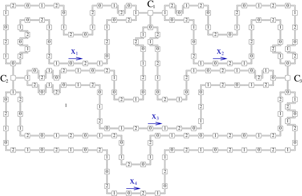
Figure 17: Replacing variables by loops (top); final polygon (bottom). Numbers 0, 1, 2 indicate the “true”, “false” and “nil” squares.

Let $N=3c=O(n^{2})$ be the total number of squares in all variable loops, and consider the placement of $N$ centers. Because the total area of the corridors is small enough, neglecting them in the following discussion changes the resulting overall average distances by not more than $O(\varepsilon^{5})$. Furthermore, we assume without loss of generality that the placement of centers is locally optimal, so any center is placed as a median of the squares closest to it. It is readily checked (making use of the constant distance between adjacent squares and the negligible area of corridors) that this allows us to assume that all centers have been placed inside of squares.

Now it is easy to estimate the overall average distance: We get an average distance of

$$D:=\frac{1}{3c}\left(\Theta(\varepsilon^{4})+\sum_{s=1}^{3c}n_{s}d\right),$$

where $n_{s}d$ is the distance of the midpoint of square $s$ to the midpoint of the closest square containing a center point; by construction, each $n_{s}$ is a nonnegative integer. As there can be at most $c$ squares with $n_{s}=0$, we conclude that $\sum_{s=1}^{3c}n_{s}\geq 2c$, with equality if and only if each square is either occupied by or next to a square with a center. For this reason, we call a square $s$ covered, if and only if $n_{s}\leq 1$. It follows from the above description that there is a distribution of centers with an average distance of $\frac{1}{3c}\left(\Theta(\varepsilon^{4})+2c\right)$, if there is a covering positioning; on the other hand, we see that the average distance must be at least $\frac{2c+1}{3c}$ if there is no covering positioning of centers.

To establish the claim of NP-hardness, we show in the following that there is a satisfying truth assignment of the instance $I$, if and only if there is a distribution of centers to squares, such that all squares are covered.

First assume that there is a covering. Consider the set of $c_{i}$ “nil” squares in a variable loop. Clearly, no two of them can be covered by the same center; by construction, no “nil” square can be covered by a center in a clause square. This implies that each variable $i$ requires precisely $c_{i}$ centers to be placed in its squares, so all $c$ centers must be placed on variable squares. As all $3c_{i}$ squares in loop $i$ must be covered by its $c_{i}$ centers, and no center can cover more than three of the squares, we conclude that each center covers precisely three of the variable squares. Thus, all centers in a variable loop must be uniformally chosen to be all “true”, all “false” or all “nil”. Finally, each clause square must be covered from one of its adjacent variable squares, which means that setting variable $i$ to the value indicated by the respective truth value satisfies the clause. Thus, all clause squares can only be satisfied if there is an overall satisfying truth assignment $I$.

Conversely, it is clear that for a satisfying truth assignment for instance $I$, placing $c_{i}$ centers in the $c_{i}$ “true” or “false” squares of variable $i$ (corresponding to the truth setting of variable $i$) yields a covering distribution of centers.

This concludes the proof. $\Box$

Note that the above proof can also be applied to the case of geodesic $L_{2}$ distances, or when minimizing the maximum distance instead of the average distance; furthermore, the underlying proof technique can also be applied to other types of location problems. For example, see [24] for a game-theoretic scenario in which two players try to claim as much area as possible by placing centers, and the second player must place all of his points after the first player has played all of her points.

8 Conclusion

In this paper, we have given the first exact algorithmic results for the Fermat-Weber problem for a continuous set of demand locations. We have shown that for $L_{1}$ distances in the plane, we can determine an optimum center in polynomial time, with the complexity ranging from $O(n)$ for the case of geodesic $L_{1}$ distances in simple polygons, to $O(n^{2})$ for straight-line distances in general polygonal regions, and $O(n^{4})$ for geodesic $L_{1}$ distances in polygons with holes. Our results rely on a careful understanding of the local optimality criteria, together with the structure and combinatorics of shortest path maps.

Extensions and Open Problems.

(1) Our results can be extended to “fixed orientation metrics” defined by any constant number of directions. (The $L_{1}$ metric is the special case in which the two fixed orientations are horizontal and vertical.) The local optimality conditions become more complex; however, the inherent algebraic complexity remains the same, for any metric whose disks are convex polygons. This extension allows one to approximate the Euclidean ($L_{2}$) case to any desired degree of precision.

(2) Our local optimality conditions generalize to the case of more general (non-uniform) nonnegative demand densities $\delta(p)$ by using the following observation. Regardless of the demand density function, any center location $Z\in P$ induces a subdivision of $P$ into $E(Z)$ and $W(Z)$, and into $N(Z)$ and $S(Z)$ by shortest-path bisectors. Then the local optimality condition on $Z$ requires that $E(Z)$ and $W(Z)$, and $S(Z)$ and $N(Z)$ are balanced in the following sense: instead of requiring that $E(Z)$ and $W(Z)$, as well as $N(Z)$ and $S(Z)$, have the same area, the balance condition is that locally optimal points $Z$ must have the integrals $\int_{p\in W(Z)}\delta(p)dp$ and $\int_{p\in E(Z)}\delta(p)dp$, and $\int_{p\in N(Z)}\delta(p)dp$ and $\int_{p\in S(Z)}\delta(p)dp$ the same. Points with these properties are called $\delta$-medians. Similar ideas can be used for describing boundary points. If, for a particular $\delta$, there is a limited number of $\delta$-medians, they can be computed in polynomial time, and it is possible to compare objective values in polynomial time, then we can determine a $\delta$-center for the given region. This includes the case in which the demand function is given by point weights in combination with a uniform demand distribution over $P$, which is a problem formulated by Wesolowsky and Love [62]. It is also easy to see that the above methods can be applied for the case in which $F\neq D$ and distances are straight-line $L_{1}$ distances. Note that geodesic distances are not well-defined in this case; however, if we use a combination of straight-line distances outside of $F$ and geodesic distances inside of $F$, our methods still apply.

(3) Our methods can also be applied in higher dimensions, by generalizing the local optimality conditions and carrying through the analysis in a very similar manner to the two-dimensional case. Figure 18 shows that a generalization of Theorem 7, however, does not hold in three-dimensional space (since any axis-parallel plane cuts the region into not more than two pieces), so we cannot use the same idea that allowed us in the two-dimensional case to exploit simplicity in achieving a better complexity than in the case of a polygon with holes. However, we can apply the technique of decomposing space into cells and studying the objective function within each cell. As in the two-dimensional case, the objective function is cubic for each coordinate, if $P$ is a polyhedral region.

Figure 18: In three-dimensional space, there may not be a feasible point that is a median of $P$ in all coordinates. In this example, the intersection of the three median planes (orthogonal to the $x$-, $y$-, and $z$-axes) is a point approximately at the center of the bounding box, not lying within the solid.

(4) Our methods for searching for local optima should be extendable to the case in which we have a constant ($k=O(1)$) number of centers, e.g., $k=2$. The centers induce a subdivision of $P$ into several “Voronoi regions”, corresponding to the set of points closest to each center. Each center must be placed optimally with respect to its region, which can be done by our methods. Thus, we are done if we have a suitable way to characterize the boundaries of Voronoi regions, which consist of a number of bisectors. While there are considerable technical details to establish, we believe that this approach will allow our results to generalize to multiple centers, and will lead to an algorithm of complexity $O(n^{ck})$, for a small constant $c$.

(5) It would be most interesting to discover an algorithm with worst-case complexity better than $O(n^{4})$ that can compute an optimal center in the geodesic $L_{1}$ distance for polygons with holes. Can we use geometric special structure to avoid examining all potential local minima in the cells of the overlay arrangement?

References

- [1] P. K. Agarwal, M. Sharir, and E. Welzl. The discrete -center problem. Discrete Comput. Geom., 20:287–305, 2000.
- [2] Y. P. Aneja and M. Parlar. Algorithms for Weber facility location in the presence of forbidden regions and/or barriers to travel. Transportation Science, 28(1):70–76, 1994.
- [3] C. Bajaj. The algebraic degree of geometric optimization problems. Discrete Comput. Geom., 3:177–191, 1988.
- [4] I. J. Balaban. An optimal algorithm for finding segment intersections. In Proc. 11th Annu. ACM Sympos. Comput. Geom., pages 211–219, 1995.
- [5] R. Batta, A. Ghose, and U. S. Palekar. Locating facilities on the Manhattan metric with arbitrarily shaped barriers and convex forbidden regions. Transportation Science, 23(1):26–36, 1989.
- [6] M. L. Brandeau and S. S. Chiu. An overview of representative problems in location research. Management Science, 35(6):645–674, 1989.
- [7] E. Carrizosa, M. Muñoz-Márquez, and J. Puerto. Location and shape of a rectangular facility in . convexity properties. Mathematical Programming, 83:277–290, 1998.
- [8] E. Carrizosa, M. Muñoz-Márquez, and J. Puerto. The Weber problem with regional demand. European Journal of Operational Research, 104:358–365, 1998.
- [9] T. M. Chan. More planar two-center algorithms. Comput. Geom. Theory Appl., 13:189–198, 1999.
- [10] R. Chandrasekaran and A. Tamir. Algebraic optimization: the Fermat-Weber location problem. Math. Program., 46(2):219–224, 1990.
- [11] B. Chazelle. Triangulating a simple polygon in linear time. Discrete Comput. Geom., 6:485–524, 1991.
- [12] B. Chazelle and H. Edelsbrunner. An optimal algorithm for intersecting line segments in the plane. J. ACM, 39(1):1–54, 1992.
- [13] R. Chen and G. Y. Handler. The conditional –center problem in the Plane. Naval Research Logistics, 40:117–127, 1993.
- [14] V. Chepoi. A multifacility location problem on median spaces. Discrete Applied Mathematics, 64:1–29, 1996.
- [15] Y.-J. Chiang and J. S. B. Mitchell. Two-point Euclidean shortest path queries in the plane. In Proc. 10th ACM-SIAM Sympos. Discrete Algorithms, pages 215–224, 1999.
- [16] J. Choi, C.-S. Shin, and K. Kim. Computing weighted rectilinear median and center set in the presence of obstacles. In Ninth Annual International Symposium on Algorithms and Computation, volume 762 of Lecture Notes Comput. Sci., pages 29–38. Springer-Verlag, 1998.
- [17] Z. Drezner. On the rectangular -center problem. Naval Res. Logist. Q., 34:229–234, 1987.
- [18] Z. Drezner. Facility Location: A Survey of Applications and Methods. Springer Series in Operations Research. Springer–Verlag, New York, 1995.
- [19] Z. Drezner. Replacing discrete demand with continuous demand. In Z. Drezner, editor, Facility Location: A Survey of Applications and Methods, Springer Series in Operations Research, chapter 2. Springer–Verlag, New York, 1995.
- [20] Z. Drezner and G. O. Wesolowsky. Optimal location of a facility relative to area demands. Naval Research Logistics Quarterly, 27:199–206, 1980.
- [21] R. Durier and C. Michelot. On the set of optimal points to the Weber problem: further results. Transportation Science, 28(2):141–149, 1994.
- [22] D. Eppstein. Faster construction of planar two-centers. In Proc. 8th ACM-SIAM Sympos. Discrete Algorithms, 1997.
- [23] S. P. Fekete and H. Meijer. On minimum stars and maximum matchings. Discrete Comput. Geom., 23:389–407, 2000.
- [24] S. P. Fekete and H. Meijer. The one-round Voronoi game replayed. In Proc. 8th Workshop Algorithms Data Struct., Lecture Notes Comput. Sci., page to appear. Springer-Verlag, 2003.
- [25] S. P. Fekete, J. S. B. Mitchell, and K. Weinbrecht. On the continuous Weber and -median problems. In Proceedings of the Sixteenth Annual ACM Symposium on Computational Geometry, Lecture Notes in Computer Science, pages 70–79, 2000.
- [26] A. J. Goldman. Optimal center location in simple networks. Transportation Science, 5:240–255, 1971.
- [27] H. W. Hamacher and S. Nickel. Classification of location problems. Location Science, 6:229–242, 1998.
- [28] J. Hershberger. A faster algorithm for the two-center decision problem. Inform. Process. Lett., 47:23–29, 1993.
- [29] J. Hershberger and S. Suri. An optimal algorithm for Euclidean shortest paths in the plane. SIAM J. Comput., 28:2215–2256, 1999.
- [30] D. S. Hochbaum and D. Shmoys. A best possible heuristic for the -center problem. Math. Oper. Res., 10:180–184, 1985.
- [31] L. K. Hua. Applications of mathematical methods for wheat harvesting. Chinese mathematics, 2:77–91, 1962.
- [32] R. Z. Hwang, R. C. T. Lee, and R. C. Chang. The slab dividing approach to solve the Euclidean -center problem. Algorithmica, 9:1–22, 1993.
- [33] O. Kariv and S. L. Hakimi. An algorithmic approach to network location problems. I: The -centers. SIAM J. Appl. Math., 37:513–538, 1979.
- [34] S. Khuller and Y. J. Sussmann. The capacitated -center problem. SIAM J. Disc. Math., 13(3):403–418, 2000.
- [35] M. T. Ko and Y. T. Ching. Linear time algorithms for the weighted tailored -partition problem and the weighted rectilinear 2-center problem under -distance. Discrete Appl. Math., 40:397–410, 1992.
- [36] M. T. Ko, R. C. T. Lee, and J. S. Chang. An optimal approximation algorithm for the rectilinear -center problem. Algorithmica, 5:341–352, 1990.
- [37] A. Kolen. Equivalence between the direct search approach and the cut approach to the rectilinear distance location problem. Operations Research, 29(3):616–620, 1981.
- [38] Y. Kusakari and T. Nishizeki. Finding a region with the minimum total distance from prescribed terminals. Algorithmica, 35:225–256, 2003.
- [39] R. C. Larson and G. Sadiq. Facility locations with the Manhattan metric in the presence of barriers to travel. Operations Research, 31(4):652–669, 1983.
- [40] D. Lichtenstein. Planar formulae and their uses. SIAM Journal on Computing, 11, 2:329–343, 1982.
- [41] R. F. Love, J. G. Morris, and G. O. Wesolowsky. Facilities Location: Models & Methods. North Hollandde Gruyter, New York, 1988.
- [42] N. Megiddo. The weighted Euclidean -center problem. Math. Oper. Res., 8(4):498–504, 1983.
- [43] N. Megiddo and A. Tamir. New results on the complexity of -center problems. SIAM J. Comput., 12:751–758, 1983.
- [44] N. Megiddo and E. Zemel. A randomized algorithm for the weighted Euclidean -center problem. J. Algorithms, 7:358–368, 1986.
- [45] P. B. Mirchandani and R. L. Francis, editors. Discrete Location Theory. Wiley, New Yorkl, 1990.
- [46] J. S. B. Mitchell. An optimal algorithm for shortest rectilinear paths among obstacles. In Abstracts 1st Canad. Conf. Comput. Geom., page 22, 1989.
- [47] J. S. B. Mitchell. A new algorithm for shortest paths among obstacles in the plane. Ann. Math. Artif. Intell., 3:83–106, 1991.
- [48] J. S. B. Mitchell. shortest paths among polygonal obstacles in the plane. Algorithmica, 8:55–88, 1992.
- [49] J. S. B. Mitchell. Shortest paths and networks. In J. E. Goodman and J. O’Rourke, editors, Handbook of Discrete and Computational Geometry, chapter 24, pages 445–466. CRC Press LLC, Boca Raton, FL, 1997.
- [50] J. S. B. Mitchell. Geometric shortest paths and network optimization. In J.-R. Sack and J. Urrutia, editors, Handbook of Computational Geometry, pages 633–701. Elsevier Science Publishers B.V. North-Holland, Amsterdam, 2000.
- [51] C. Papadimitriou. Worst case and probabilistic analysis of a geometric location problem. SIAM J. Computing, 3:542–557, 1981.
- [52] F. Plastria. Continuous location problems. In Z. Drezner, editor, Facility Location: A Survey of Applications and Methods, Springer Series in Operations Research, chapter 11. Springer–Verlag, New York, 1995.
- [53] R. Pollack, M. Sharir, and G. Rote. Computing of the geodesic center of a simple polygon. Discrete Comput. Geom., 4:611–626, 1989.
- [54] P. Rosenstiehl and R. E. Tarjan. Rectilinear planar layouts and bipolar orientations of planar graphs. Discrete and Computational Geometry, 1:343–353, 1986.
- [55] M. Sharir. A near-linear algorithm for the planar -center problem. Discrete Comput. Geom., 18:125–134, 1997.
- [56] M. Sharir and E. Welzl. Rectilinear and polygonal -piercing and -center problems. In Proc. 12th Annu. ACM Sympos. Comput. Geom., pages 122–132, 1996.
- [57] H. D. Sherali and F. L. Nordai. NP-hard, capacitated, balanced -median problems on a chain graph with a continuum of link demands. Mathematics of Operations Research, 13:32–49, 1988.
- [58] A. Tamir. On the solution value of the continuous -center location problem on a graph. Mathematics of Operations Research, 12:340–349, 1987.
- [59] A. Weber. Über den Standort der Industrien, 1. Teil: Reine Theorie des Standortes. Tübingen, Germany, 1909.
- [60] K. Weinbrecht. Kontinuierliche Standortprobleme in Polygonen. PhD thesis, Universität zu Köln, 1999.
- [61] G. Wesolowsky. The Weber problem: History and perspective. Location Science, 1:5–23, 1993.
- [62] G. O. Wesolowsky and R. F. Love. Location of facilities with rectangular distances among point and area destinations. Naval Research Logistics Quarterly, 18:83–90, 1971.
- [63] G. O. Wesolowsky and R. F. Love. The optimal location of new facilities using rectangular distances. Operations Research, 19:124–130, 1971.
- [64] G. O. Wesolowsky and R. F. Love. A nonlinear approximation method for solving a generalized rectangular distance Weber problem. Management Science, 11:656–663, 1972.
- [65] E. Zemel. Probabilistic analysis of geometric location problems. SIAM J. Alg. and Discrete Methods, 6:189–200, 1985.