Results on the quantitative $\mu$-calculus qM$\mu$

Abstract

The $\mu$-calculus is a powerful tool for specifying and verifying transition systems, including those with both demonic (universal) and angelic (existential) choice; its quantitative generalisation qM$\mu$ [17, 29, 9] extends that to probabilistic choice.

We show here that for a finite-state system the logical interpretation of qM$\mu$, via fixed-points in a domain of real-valued functions into $[0,1]$, is equivalent to an operational interpretation given as a turn-based gambling game between two players.

The equivalence sets qM$\mu$ on a par with the standard $\mu$-calculus, in that it too can benefit from a solid interface linking the logical and operational frameworks.

The logical interpretation provides direct access to axioms, laws and meta-theorems. The operational, game- based interpretation aids the intuition and continues in the more general context to provide a surprisingly practical specification tool — meeting for example Vardi’s challenge to “figure out the meaning of $\textsf{AF}\,\textsf{AX}\,p$” as a branching-time formula.

A corollary of our proofs is an extension of Everett’s singly-nested games result in the finite turn-based case: we prove well-definedness of the minimax value, and existence of fixed memoriless strategies, for all qM$\mu$ games/formulae, of arbitrary (including alternating) nesting structure.

1 Introduction

The standard $\mu$-calculus, introduced by Kozen [20], extends Boolean dynamic program logic by the introduction of least ($\mu$) and greatest ($\nu$) fixed-point operators. Its proof system is applicable to both infinite and finite state spaces; recent results [47] have established a complete axiomatisation; and it can be specialised to temporal logic. Thus it has a simple semantics, and a proof theory.

But its operational significance can be more elusive: general $\mu$-calculus expressions can be difficult to use, because in all but the simplest cases they are not easy on the intuition. Alternating fixed points can be especially intricate; and even the more straightforward (alternation-free) temporal subset has properties (particularly “branching-time properties”) that are notoriously difficult to specify, as Vardi points out [45].

Stirling’s “two-player-game” interpretation alleviates this problem by providing an alternative and complementary operational view [43].

The quantitative modal $\mu$-calculus acts over probabilistic transition systems, extending the standard axioms from Boolean- to real values; and it would benefit just as much from having two complementary interpretations. Our goal in this paper is to identify them, and to give the proof of their equivalence, over a finite state space: one interpretation (defined earlier [29, 17, 9]) generalises Kozen’s by lifting it from the Booleans into the reals; the other (defined here) generalises Stirling’s.

Our principal contribution here is thus the definition of the Stirling-style but quantitative interpretation, and the proof of its equivalence to the Kozen-style quantitative interpretation. We show also that memoriless strategies suffice, for both interpretations, again when the state space is finite.

The Kozen-style quantitative interpretation is based on our earlier extension [19, 34] of Dijkstra/Hoare logic to probabilistic/demonic programs (corresponding to the $\forall$ modality): it is a real-valued logic based on “greatest pre-expectations” of random variables, rather than weakest preconditions of predicates. It can express the specific “probability of achieving a postcondition,” since the probability of an event is the expected value of its characteristic function, but it applies more generally to other cost-based properties besides. Although the specific approach, i.e. with its explicit probabilities — may be more intuitive, the extra generality of a full quantitative logic seems necessary for compositionality [24].

Converting predicates “wholesale” from Boolean- to real-valued state functions — due originally to Kozen [18] and extended by us to include demonic (universal) [34] and angelic (existential) [22] nondeterminism — contrasts with probabilistic logics using “threshold functions” [3, 35] that mix Boolean and numeric arguments: the uniformity in our case means that standard Boolean identities in branching-time temporal logic [2] suggest corresponding quantitative laws for us [30], and so we get a powerful collection of algebraic properties “for free.” The logical “implies” relation between Booleans is replaced by the standard “$\leq$” order on the reals; false and true become 0 and 1; and fixed points are then associated with monotonic real- rather than Boolean-valued functions. The resulting arithmetic logic is applicable to a restricted class of real-valued functions, and we recall its definition in Sec. 3.

Our Stirling-style quantitative interpretation is operational, and is based on his earlier strategy-based game metaphor for the standard $\mu$-calculus. In our richer context, however, we must distinguish nondeterministic choice — both demonic and angelic — from probabilistic choice: the former continues to be represented by the two players’ strategies; but the latter is represented by the new feature that we make the players gamble. In Sec. 4 we set out the details.

In Sec. 5 we give a worked example of the full use of the quantitative aspects of the calculus, beyond simply calculating probabilities.

The main mathematical result of this paper is given in Sec. 6, though much of the detail is placed in the appendices.

Stirling showed that for non-probabilistic formulae the Boolean value of the Kozen interpretation corresponds to the existence of a winning strategy in his game interpretation. In our case, strategies in the game must become “optimal” rather than “winning”; and the correspondence is now between a formula’s value (since it denotes a real number, in the Kozen interpretation) and the expected winnings from the zero-sum gambling game (of the Stirling interpretation). Since the gambling game described by a formula is a “minimax,” we must show it to be well-defined (equal to the “maximin”): in fact we show that both the minimax and the maximin of the game are equal to the Kozen-style denotation of the formula that generated it.

We also prove that memoriless strategies suffice.

Both proofs apply only to finite state spaces.

The benefit of our proved equivalence is to set the quantitative $\mu$-calculus on a par with standard $\mu$-calculus in that a suitable form of “logical validity” corresponds exactly to an operational interpretation. As with standard $\mu$-calculus, a specifier can use the operational semantics to build his intuitions into a game, and can then use the general features of the logic — whose soundness has been proved relative to the logical semantics — to prove properties about the specific application. For example, the sublinearity [34] of qM$\mu$ — the quantitative generalisation of the conjunctivity of standard modal algebras — has been used in its quantitative temporal subset qTL to prove a number of algebraic laws corresponding to those holding in standard branching-time temporal logic [30].

Preliminary experiments have shown that the proof system is very effective for unravelling the intricacies of distributed protocols [39, 31]. Moreover it provides an attractive proof framework for Markov decision processes [32, 11] — and indeed many of the problems there have a succinct specification as $\mu$-calculus formulae, as the example of Sec. 5 illustrates. In “reachability-style problems” [7], proof-theoretic methods based on the logic presented here have produced very direct arguments related to the abstraction of probabilities [33], and even more telling is that the logic is applicable even in infinite state spaces [7]. All of which is to suggest that further exploration of qM$\mu$ will continue to be fruitful.

In the following we shall assume generally that $S$ is a countable state space (though for the principal result we restrict to finiteness, in Sec. 6). If $f$ is a function with domain $X$ then by $f.x$ we mean $f$ applied to $x$, and $f.x.y$ is $(f.x).y$ where appropriate; functional composition is written with $\circ$, so that $(f\mbox{\scriptsize$\circ$}g).x=f.(g.x)$. We denote the set of discrete probability sub-distributions over a set $X$ by $\overline{X}$: it is the set of functions from $X$ into the real interval $[0,1]$ that sum to no more than one; and if $A$ is a random variable with respect to some probability space, and $\delta$ is some probability sub-distribution, we write $\int_{\delta}A$ for the expected value of $A$ with respect to $\delta$. In the special case that $\delta$ is in $\overline{X}$ and $A$ is a bounded real-valued function on $X$, in fact $\int_{\delta}A$ is equal to $\sum_{s:S}A.s\times\delta.s$.

2 Probabilistic transition systems and $\mu$-calculus

In this section we set out the logical language, together with some details about the probabilistic systems over which the formulae are to be interpreted.

Formulae in the logic (in positive form) are constructed as follows:

$$\phi~{}~{}~{}\mathrel{\hat{=}}~{}~{}~{}X\mid\textsf{A}\mid\langle\textsf{K}\rangle\phi\mid[\textsf{K}]\phi\mid\phi_{1}\sqcap\phi_{2}\mid\phi_{1}\sqcup\phi_{2}\mid\phi_{1}\lhd\textsf{G}\rhd\phi_{2}\mid(\mu X\mathrel{\mbox{\boldmath$\cdot$}}\phi)\mid(\nu X\mathrel{\mbox{\boldmath$\cdot$}}\phi)~{}.$$

• Variables $X$ are of type $S\rightarrow[0,1]$, and are used for binding fixed points.

• Terms A stand for fixed functions in $S\rightarrow[0,1]$.

• Terms K represent finite non-empty sets of probabilistic state-to-state transitions in ${\cal R}.S$ (see below), with $\langle\cdot\rangle$ and $[\cdot]$ forming respectively angelic- (existential-) and demonic (universal) modalities from them.

• Terms G describe Boolean functions of $S$, used in $\lhd~{}\textrm{(``if'')}~{}\textsf{G}~{}\rhd~{}\textrm{(``else'')}$ style [16].

It is well known that such formulae can be used to express complex path-properties of computational sequences. In this paper we interpret the formulae over sequences based on generalised probabilistic transitions in what we call ${\cal R}.S$, the functions $t$ in $S\rightarrow\overline{S_{\$}}$ where $S_{\$}$ is just the state space $S$ with a special “payoff” state $\$$ adjoined. Thus $\overline{S_{\$}}$ is the set of sub-distributions over that, so that the elements $t$ of ${\cal R}.S$ give the probability of passage from initial $s$ to final (proper) $s^{\prime}$ as $t.s.s^{\prime}$; any deficit $1-\sum_{s^{\prime}}t.s.s^{\prime}$ is interpreted as the probability of an immediate halt with payoff

$$t.s.\$/(1-\sum_{s^{\prime}\colon S}t.s.s^{\prime})~{}.$$ (1)

See Fig. 1 for an example.

This formulation of the payoff — i.e. “pre-divided” by its probability of occurrence — has three desirable properties. The first is that the probabilistically expected halt-and-payoff is just $t.s.\$$, i.e. is given directly by $t$. The second property is that we can consider the probabilities of outcomes from $s$ to sum to one exactly (rather than no more than one), since any deficit is “soaked up” in the probability of transit to payoff, which simplifies our operational interpretation.

The relational element $\left(\begin{array}[]{rcl}s&\stackrel{{\scriptstyle 1/4}}{{\longrightarrow}}&\textsf{H}\\ s&\stackrel{{\scriptstyle 1/4}}{{\longrightarrow}}&\textsf{T}\\ s&\stackrel{{\scriptstyle 2/5}}{{\longrightarrow}}&\textrm{\$}\end{array}\right)$ in ${\cal R}.S$, with its deficit of $1/10$, denotes the transition shown,

in which the transition probabilities now sum to one. In particular, the probability of transition to $\$$ is $1/2$, which makes the expected immediate payoff equal to $1/2\times 0.80=2/5$ as given explicitly in the relation.

Since $\textsf{H},\textsf{T}$ are states, they may lead further: no matter where they lead, however, the expected reward of the subtrees rooted there cannot exceed one, and so our encoding ensures both that the transition probabilities from $s$ sum to one exactly (since the probability of transition $s\mapsto\$$ is $1/2=1-(1/4+1/4)$ by definition), and that the expected reward from this tree (rooted at $s$) cannot exceed one either (since the actual reward $\$0.80$ is defined just so that $2/5=0.8\times 1/2$ will hold).

The tree does not continue on from the payoff state $\$0.80$.

More generally, a “normal” transition, i.e. with $\sum_{i}p_{i}=1$, can effectively be “$\alpha$-discounted” by using the elements $(s\stackrel{{\scriptstyle\alpha p_{i}~{}}}{{\longrightarrow}}s_{i},s\stackrel{{\scriptstyle 0}}{{\longrightarrow}}\$)$ or $(s\stackrel{{\scriptstyle\alpha p_{i}~{}}}{{\longrightarrow}}s_{i},s\stackrel{{\scriptstyle 1{-}\alpha}}{{\longrightarrow}}\$)$.

Figure 1: Example of payoff-state encoding

The third property is that transitions preserve one-boundedness in the following sense. Define the set of expectations ${\cal E}S$ (over $S$) to be the set of one-bounded functions $S\rightarrow[0,1]$. If $A$ in ${\cal E}S$ gives a “post-expectation” $A.s^{\prime}$ expected to be realised at state $s^{\prime}$ after transition $t$, then the “pre-expectation” at $s$ before transition $t$ is

$$t.s.\$+\int_{t.s}A~{},\quad\parbox[t]{200.0003pt}{where the sub-distribution $t.s$ under $\int$ is restricted to states in $S$ proper.}$$

It is the expected value realised by making transition $t$ from $s$ to $s^{\prime}$ or possibly $\$$, taking $A.s^{\prime}$ in the former case and (1) in the latter. That this pre-expectation is also one-bounded, i.e. is in ${\cal E}S$, allows us to confine our work to the real interval $[0,1]$ throughout.

Hence computation trees can be constructed by “pasting together” applications of transitions $t_{0},t_{1},\ldots$ drawn from ${\cal R}.S$, with branches to $\$$ being tips. The probabilities attached to the individual steps then generate a distribution over computational paths (which is defined by the sigma-algebra of extensions of finite sequences, a well-known construction [12]).

We use the relation $\leq$ — “everywhere no more than” between expectations (thus replacing “implies”):

$$A\leq A^{\prime}~{}~{}~{}\textrm{iff}~{}~{}~{}(\forall s\colon S\mathrel{\mbox{\boldmath$\cdot$}}A.s\leq A^{\prime}.s)~{}.$$

In our interpretations we will use valuations in the usual way. Given a formula $\phi$, a valuation ${\cal V}$ does four things: (i) it maps each A in $\phi$ to a fixed expectation in ${\cal E}S$; (ii) it maps each K to a fixed, non-empty finite set of probabilistic transitions in ${\cal R}.S$; (iii) it maps each G to a predicate over $S$; and (iv) it keeps track of the current instances of “unfoldings” of fixed points, by including mappings for bound variables $X$. (For notational economy, in (iv) we are allowing ${\cal V}$ to take over the role usually given to a separate “environment” parameter.)

We make one simplification to our language, without compromising expressivity. Because the valuation ${\cal V}$ assigns finite sets to all occurrences of K, we can replace each modality $\langle\textsf{K}\rangle\phi$ (resp. $[\textsf{K}]\phi$) by an explicit maxjunct $\sqcup_{\textsf{k}\colon\textsf{K}}\{\textsf{k}\}\phi$ (resp. minjunct $\sqcap_{\textsf{k}\colon\textsf{K}}\{\textsf{k}\}\phi$) of (symbols k denoting) transitions $k$ in the set (denoted by) K. We do this because our interpretations conveniently do not distinguish between $\langle\textsf{K}\rangle$ or $[\textsf{K}]$ when K is a singleton set.

In the rest of this paper we shall therefore use the reduced language given by

$$\phi~{}~{}~{}\mathrel{\hat{=}}~{}~{}~{}X\mid\textsf{A}\mid\{\textsf{k}\}\phi\mid\phi_{1}\sqcap\phi_{2}\mid\phi_{1}\sqcup\phi_{2}\mid\phi_{1}\lhd\textsf{G}\rhd\phi_{2}\mid(\mu X\mathrel{\mbox{\boldmath$\cdot$}}\phi)\mid(\nu X\mathrel{\mbox{\boldmath$\cdot$}}\phi)~{}.$$

We replace (ii) above in respect of ${\cal V}$ by: (ii’) it maps each occurrence of $\{\textsf{k}\}$ to a probabilistic transition in ${\cal R}.S$.

3 Denotational interpretation: qM$\mu$ generalises Kozen’s logic

In this section we recall how the quantitative logic for nondeterministic/probabilistic sequential programs [19, 34] — from which we inherit the use of expectations, and the semantic definition $|\!|\{\textsf{k}\}\phi|\!|$ below — leads to a quantitative generalisation of Kozen’s logical interpretation of $\mu$-calculus, suitable for probabilistic transition systems.

Let $\phi$ be a formula and ${\cal V}$ a valuation. We write $|\!|\phi|\!|_{{\cal V}}$ for its meaning, an expectation in ${\cal E}S$ determined by the rules given in Fig. 2. Part of the contribution of our previous work [29, 30] is summarised in the following lemma.

1. $|\!|X|\!|_{{\cal V}}~{}~{}~{}\mathrel{\hat{=}}~{}~{}~{}{\cal V}.X$  .

2. $|\!|\textsf{A}|\!|_{{\cal V}}~{}~{}~{}\mathrel{\hat{=}}~{}~{}~{}{\cal V}.\textsf{A}$  .

3. $|\!|\{\textsf{k}\}\phi|\!|_{{\cal V}}.s~{}~{}~{}\mathrel{\hat{=}}~{}~{}~{}{\cal V}.\textsf{k}.s.\$~{}+~{}\int_{\makebox[0.0pt][l]{\raisebox{-3.61664pt}{\scriptsize${\cal V}.\textsf{k}.s$}}}~{}|\!|\phi|\!|_{{\cal V}}$  .

5. $|\!|\phi^{\prime}\sqcap\phi^{\prime\prime}|\!|_{{\cal V}}.s~{}~{}~{}\mathrel{\hat{=}}~{}~{}~{}|\!|\phi^{\prime}|\!|_{{\cal V}}.s~{}\textsf{min}~{}|\!|\phi^{\prime\prime}|\!|_{{\cal V}}.s$  ; and
   $|\!|\phi^{\prime}\sqcup\phi^{\prime\prime}|\!|_{{\cal V}}.s~{}~{}~{}\mathrel{\hat{=}}~{}~{}~{}|\!|\phi^{\prime}|\!|_{{\cal V}}.s~{}\textsf{max}~{}|\!|\phi^{\prime\prime}|\!|_{{\cal V}}.s$  .

7. $|\!|\phi^{\prime}\lhd\textsf{G}\rhd\phi^{\prime\prime}|\!|_{{\cal V}}.s~{}~{}~{}\mathrel{\hat{=}}~{}~{}~{}|\!|\phi^{\prime}|\!|_{{\cal V}}.s~{}\textrm{\text@underline{if}}~{}({\cal V}.\textsf{G}.s)~{}\textrm{\text@underline{else}}~{}|\!|\phi^{\prime\prime}|\!|_{{\cal V}}.s$  .

9. $|\!|(\mu X\mathrel{\mbox{\boldmath$\cdot$}}\phi)|\!|_{{\cal V}}~{}~{}~{}\mathrel{\hat{=}}~{}~{}~{}(\mathop{\sf lfp}x\mathrel{\mbox{\boldmath$\cdot$}}|\!|\phi|\!|_{{\cal V}_{[X\mapsto x]}})$   where by $(\mathop{\sf lfp}x\mathrel{\mbox{\boldmath$\cdot$}}\textit{exp})$ we mean the least fixed-point of the function $(\lambda x\mathrel{\mbox{\boldmath$\cdot$}}\textit{exp})$.

10. $|\!|(\nu X\mathrel{\mbox{\boldmath$\cdot$}}\phi)|\!|_{{\cal V}}~{}~{}~{}\mathrel{\hat{=}}~{}~{}~{}(\mathop{\sf gfp}x\mathrel{\mbox{\boldmath$\cdot$}}|\!|\phi|\!|_{{\cal V}_{[X\mapsto x]}})$  .

Note that in the valuation ${\cal V}_{[X\mapsto x]}$, the variable $X$ is mapped to the expectation $x$.

Figure 2: Kozen-style denotational semantics for qM$\mu$

Lemma 1

The quantitative logic qM$\mu$ is well-defined —  For any $\phi$ in the language, and valuation ${\cal V}$, the interpretation $|\!|\phi|\!|_{{\cal V}}$ is a well-defined expectation in ${\cal E}S$.

Proof

Structural induction: arithmetic, that our formulae express only monotone functions, and that $({\cal E}S$, $\leq)$ is a complete partial order. (Recall that ${\cal E}S$ is $[0,1]$-bounded.)

4 Operational interpretation: qM$\mu$ generalises Stirling’s game

In this section we give an alternative account of formulae $\phi$ (of the reduced language), in terms of a generalisation of Stirling’s turn-based game [43]. The game is between two players, to whom we refer as Max and Min. As in Sec. 3, we assume a probabilistic transition system ${\cal R}.S$ and a valuation ${\cal V}$. Play progresses through a sequence of game positions, each of which is either a pair $(\phi,s)$ where $\phi$ is a formula and $s$ is a state in $S$, or a single $(y)$ for some real-valued payoff $y$ in $[0,1]$. Following Stirling, we will use the idea of “colours” to handle repeated returns to a fixed point.

A sequence of game positions is called a game path and is of the form $(\phi_{0},s_{0}),~{}(\phi_{1},s_{1}),\ldots$ with (if finite) a payoff position $(p_{n})$ at the end. The initial formula $\phi_{0}$ is the given $\phi$, and $s_{0}$ is an initial state in $S$. A move from position $(\phi_{i},s_{i})$ to $(\phi_{i+1},s_{i+1})$ or to $(y)$ is specified by the rules of Fig. 3.

If the current game position is $(\phi_{i},s_{i})$, then play proceeds as follows:

1. Free variables $X$ do not occur in the game — their role is taken over by “colours” (see Cases 6–8 below.).

2. If $\phi_{i}$ is A then the game terminates in position $(y)$ where $y={\cal V}.\textsf{A}.s_{i}$.

4. if $\phi_{i}$ is $\{\textsf{k}\}\phi$ then the distribution ${\cal V}.\textsf{k}.s_{i}$ is used to choose either a next state $s^{\prime}$ in $S$ or possibly the payoff state $\$$. If a state $s^{\prime}$ is chosen, then the next game position is $(\phi,s^{\prime})$; if $\$$ is chosen, then the next position is $(y)$, where $y$ is the payoff ${\cal V}.\textsf{k}.s.\$/(1-\sum_{s^{\prime}\colon S}{\cal V}.\textsf{k}.s.s^{\prime})$, and the game terminates.

6. If $\phi_{i}$ is $\phi^{\prime}\sqcap\phi^{\prime\prime}$ (resp. $\phi^{\prime}\sqcup\phi^{\prime\prime}$) then Min (resp. Max) chooses one of the minjuncts (maxjuncts): the next game position is $(\phi,s_{i})$, where $\phi$ is the chosen ’junct $\phi^{\prime}$ or $\phi^{\prime\prime}$.

7. If $\phi_{i}$ is $\phi^{\prime}\lhd\textsf{G}\rhd\phi^{\prime\prime}$, the next game position is $(\phi^{\prime},s_{i})$ if ${\cal V}.\textsf{G}.s_{i}$ holds, and otherwise it is $(\phi^{\prime\prime},s_{i})$.

9. If $\phi_{i}$ is $(\mu X\mathrel{\mbox{\boldmath$\cdot$}}\phi)$ then a fresh colour ${\sf C}$ is chosen and is bound to the formula $\phi_{[X\mapsto{\sf C}]}$ for later use; the next game position is $({\sf C},s_{i})$.

10. If $\phi_{i}$ is $(\nu X\mathrel{\mbox{\boldmath$\cdot$}}\phi)$, then a fresh colour ${\sf C}$ is chosen and bound as for $\mu$.

12. If $\phi_{i}$ is a colour ${\sf C}$, then the next game position is $(\phi,s_{i})$, where $\Phi$ is the formula bound previously to ${\sf C}$.

The game begins with a closed formula — refer Item 1. above.

Infinite games result in there being a single colour ${\sf C}$ that occurs infinitely often; finite games end in a payoff $(y)$ for $0\leq y\leq 1$.

Figure 3: Rules for playing probabilistic formula-game.

A game path is said to be valid if it can occur as a sequence according to the above rules. Note that along any game path at most one colour can appear infinitely often:

Lemma 2

All valid game paths are either finite, terminating at some payoff $(y)$, or infinite; if infinite, then exactly one colour appears infinitely often.

Proof

Stirling [43].

To complete the description of the game, one would normally give the winning/losing conditions. Here however we are operating over real- rather than Boolean values, and we speak of the “value” of the game. In the choices $\phi^{\prime}\sqcup\phi^{\prime\prime}$ (resp. $\phi^{\prime}\sqcap\phi^{\prime\prime}$) player Max (resp. Min) follows a strategy in which he tries to maximise (minimise) a real-valued “payoff” associated with the game, defined as follows.

Definition 1

Value of a path — The value of a path is determined by a fixed function Val defined by cases as follows:

1. The path $\pi$ is finite, terminating in a game state $(y)$; in this case the value $\textit{Val}.\pi$ is $y$.

2. The path $\pi$ is infinite and there is a colour ${\sf C}$ appearing infinitely often that was generated by a greatest fixed-point $\nu$; in this case $\textit{Val}.\pi$ is $1$.

3. The path $\pi$ is infinite and there is a colour ${\sf C}$ appearing infinitely often that was generated by a least fixed-point $\mu$; in this case $\textit{Val}.\pi$ is $0$.

In Sec. 6.1 we make precise this notion of “value of a game,” and its interaction with strategies.

5 Worked example: investing in the futures market

5.1 Describing a game

Typical properties of probabilistic systems are usually cost-based, and to illustrate that we give an example involving money. Concerning general expected values, it lies strictly outside the scope of “plain” probabilistic temporal logic.

An investor $I$ has been given the right to make an investment in “futures,” a fixed number of shares in a specific company that he can reserve on the first day of any month he chooses. Exactly one month later, the shares will be delivered and will collectively have a market value on that day — he can sell them then if he wishes.

His problem is to decide when to make his reservation so that the subsequent sale has maximum value.

The details are as follows:

1. The market value $v$ of the shares is a whole number of dollars between $0 and $10 inclusive; it has a probability $p$ of going up by $1 in any month, and $1{-}p$ of going down by $1 — but it remains within those bounds. The probability $p$ represents short-term market uncertainty.

2. Probability $p$ itself varies month-by-month in steps of $0.1$ between zero and one: when $v$ is less than $5 the probability that $p$ will rise is $2/3$; when $v$ is more than $5 the probability of $p$’s falling is $2/3$; and when $v$ is $5 exactly the probability is $1/2$ of going either way. The movement of $p$ represents investors’ knowledge of long-term “cyclic second-order” trends.

3. There is a cap $c$ on the value of $v$, initially $10, which has probability $1/2$ of falling by $1 in any month; otherwise it remains where it is. (This modifies Item 1. above.) The “falling cap” models the fact that the company is in a slow decline.

4. If in a given month the investor does not reserve, then at the very next month he might find he is temporarily barred from doing so. But he cannot be barred two months consecutively.

5. If he never reserves, then he never sells and his return is thus zero.

If it were not for Item 3., the investor’s strategy would be the obvious “wait until $v\geq 9\land p=1$ — however long that takes — and make a reservation then.” But the falling cap defeats that, effectively discounting the payoff as time passes. Below we consider more sophisticated strategies that take that into account.

The situation is summed up by the transition system set out in Fig. 4:

• During each month there are three purely probabilistic actions that occur, and their compounded effects determine a transition $m$, which we will call month in our formula (to come);

• At the beginning of each month, the investor makes a maximising (angelic) choice of whether to reserve; but, if he does not, then

• At the beginning of the next month, there is a minimising (demonic) choice of whether he is barred.

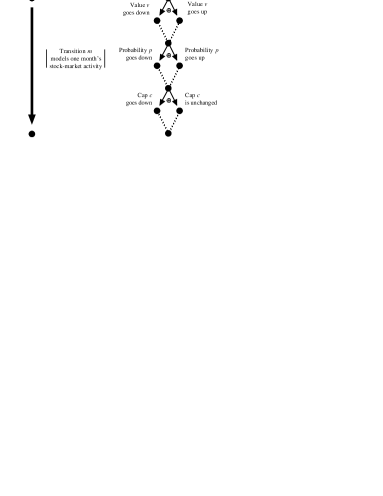
The thick arrow, “exploded” on the right, represents the effect of one month’s stock-market activity: symbol $\oplus$ labels the probabilistic choices it entails. The share value $v$ may rise or fall, according to $p$; probability $p$ itself may rise or fall, according to long-term trends; and the capped value $c$ of the stock may fall.

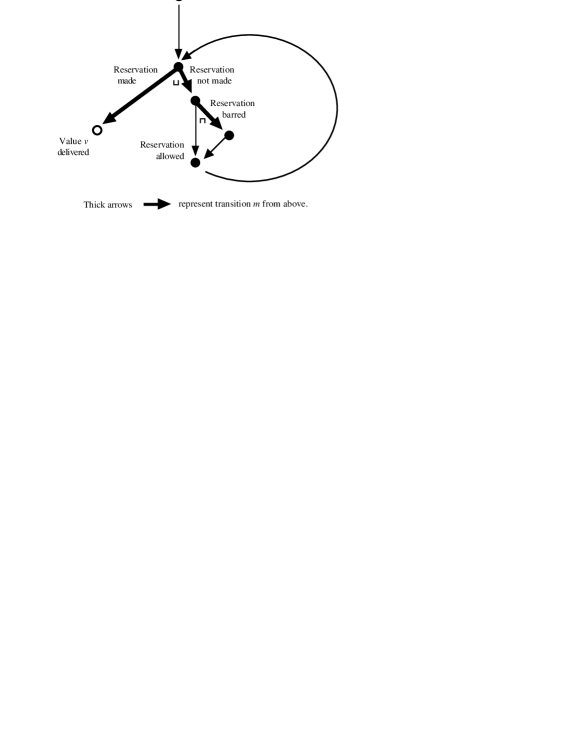
This represents the non-deterministic choices available to the investor (maximising player) and the market (minimising player). Symbol $\sqcup$ represents the investor’s choice; symbol $\sqcap$ represents the market’s choice.

(The probabilistic choices occur “within” the thick arrows.)

Figure 4: Futures trading on the stock market: example.

The utility of our game interpretation in Sec. 4 is that we can easily use the intuition it provides to write a formula describing the above system. The state space is $(v,p,c)$, and we use a transition

$$\begin{array}[]{l@{\quad}c@{\quad}l}m&\mathrel{\hat{=}}&\begin{array}[t]{@{}l}v\colon=\,(v+1)\sqcap c~{}~{}\mathbin{\makebox[0.0pt]{~{}}_{p}\oplus}~{}~{}(v-1)\sqcup 0;\\ \\ \begin{array}[]{@{}l@{~~}c@{~~}l@{~~}l}\textbf{if}\hfil~{}~{}&v<5\hfil~{}~{}&\textbf{then}\hfil~{}~{}&p\colon=\,(p{+}0.1)\sqcap 1~{}\mathbin{\makebox[0.0pt]{~{}}_{2/3}\oplus}~{}(p{-}0.1)\sqcup 0\\ \textbf{elsif}\hfil~{}~{}&v>5\hfil~{}~{}&\textbf{then}\hfil~{}~{}&p\colon=\,(p{-}0.1)\sqcup 0~{}\mathbin{\makebox[0.0pt]{~{}}_{2/3}\oplus}~{}(p{+}0.1)\sqcap 1\\ \textbf{else}\hfil~{}~{}&\hfil~{}~{}&\hfil~{}~{}&p\colon=\,(p{-}0.1)\sqcup 0~{}\mathbin{\makebox[0.0pt]{~{}}_{1/2}\oplus}~{}(p{+}0.1)\sqcap 1\\ \textbf{fi};\hfil~{}~{}\end{array}\\ \\ c\colon=\,(c{-}1)\sqcup 0~{}~{}\mathbin{\makebox[0.0pt]{~{}}_{1/2}\oplus}~{}~{}c\end{array}\end{array}$$

to capture the effect of the large arrows.

We can then use our (reduced) logical language to describe the surrounding angelic and demonic choices, including the “loop back” (fixed point) which gives value zero (i.e. $\mu$) if it never terminates. Using month to denote $m$, and a constant expectation Sold to denote the function $\widehat{v}$ returning just the $v$ component of the state, we would write our formula as

$$\textit{Game}~{}~{}~{}\mathrel{\hat{=}}~{}~{}~{}(\mu X\mathrel{\mbox{\boldmath$\cdot$}}\{\textsf{month}\}\textsf{Sold}~{}\sqcup~{}\{\textsf{month}\}(X\sqcap\{\textsf{month}\}X))~{}.$$ (2)

5.2 Playing the game

Using the game interpretation, we can generate a probabilistic tree from the transition system in Fig. 4 by duplicating nodes with multiple incoming arcs (as in month), “unfolding” back-loops, and making minimising or maximising choices as they are encountered. In this example, at each unfolding both the investor $I$ (making $\sqcup$ choices) and the stock market $M$ (making $\sqcap$ choices whether to impose a bar) need to choose between two ongoing branches — and their choice could be different each time they revisit their respective decision points. Each of $I,M$ will be using a strategy.

For example (recalling Footnote 16), the investor $I$’s strategy (maximising, he hopes) for dealing with the falling cap might be

wait until the share value $$v c$$ (rising) meets the cap (falling), and reserve then. (3)

Waiting for $v$ to rise is a good idea, but when it has met the cap $c$ there is clearly no point in waiting further.

And $M$’s strategy (minimising, the investor fears) might be

bar the investor, if possible, whenever the shares’ probability $$p$$ of rising exceeds 1/2. (4)

In general, let $\sigma_{I}$ and $\sigma_{M}$ be sequences (possibly infinite) of choices, like the above, that $I$ and $M$ might make. When they follow those sequences, the game-tree they generate determines a probability distribution over valid game paths [12]. Anticipating the next section, let $[\![\phi]\!]_{{\cal V}}^{\sigma_{I},\sigma_{M}}$ denote that path distribution as generated by $I$ and $M$’s choices. We can now describe $I$’s actual payoff as an expected value

$$Y.\sigma_{I}.\sigma_{M}~{}~{}~{}\mathrel{\hat{=}}~{}~{}~{}\int_{\makebox[0.0pt][l]{\raisebox{-3.61664pt}{\scriptsize$[\![\phi]\!]_{{\cal V}}^{\sigma_{I},\sigma_{M}}$}}}~{}\textrm{``the $v$-component of the final state''}~{},$$ (5)

with the understanding that the random variable in the integral’s body yields zero if in fact there is no final state (because of an infinite path).

In some cases, the choices made by $I$ and $M$ can be memoriless, in the sense that in identical situations (identical values of $v,p,c$ in this case, and the same position in the transition system) they will always make the same choice. Both (3) and (4) above are memoriless.

Memoriless strategies are particularly important for the efficient computation of expected payoffs [11], and in Sec. 6 we show that they suffice for analysis of qM$\mu$ formulae when the state space is finite — that is, informally, the players gain no advantage by remembering where they have been.

5.3 The value of the game

As is usual in game theory, when the actual strategies of the two players are unknown, we define the value of the game to be the the minimax over all strategy sequences of the expected payoff — but it is well-defined only when it is the same as the maximin, i.e. when in the notation of (5) we have

$$\sqcup_{\sigma_{I}}\sqcap_{\sigma_{M}}Y.\sigma_{I}.\sigma_{M}~{}~{}~{}=~{}~{}~{}\sqcap_{\sigma_{M}}\sqcup_{\sigma_{I}}Y.\sigma_{I}.\sigma_{M}~{}.$$

The equivalence proved in Thm. 6.1, to come, tells us that such games’ values are indeed well-defined, and that although we use the game interpretation to write down the formulae, we can use the logical interpretation $|\!|\textit{Game}|\!|_{{\cal V}}$ to reason about their values. Sometimes, as in this simple case, we can use the logical interpretation to calculate an approximation directly.

Although the details of month are (deliberately) slightly messy, the structure of the overall formula Game has been chosen (also deliberately) to be fairly simple, and as such the fixed point can be approximated by iterating the function

$$(\lambda X\mathrel{\mbox{\boldmath$\cdot$}}m\,\mbox{\scriptsize$\circ$}\,\widehat{v}~{}\sqcup~{}m.(X\sqcap m.X))$$

beginning from the constant “bottom” function that is zero everywhere on the state space.

Carrying out that calculation shows for example that if $p$ is initially $0.5$ and the cap $c$ is 10, then the optimal expected sale-value for the investor is

$$\begin{array}[]{l|r|r|r|r|r|r|r|r|r|r|r|}\cline{2-12}\cr\textit{\scriptsize initial share value:~{}~{}}&0&1&2&3&4&5&6&7&8&9&10\\ \cline{2-12}\cr\textit{\scriptsize optimal expected sale:~{}~{}}&4.16&4.30&4.55&4.88&5.24&5.52&6.00&7.00&8.00&9.00&9.50\\ \cline{2-12}\cr\end{array}$$ (6)

Even when the share value is only “moderately high,” we thus see there is nothing to be gained by waiting, since the cap is likely to drop. For low initial values, however, some benefit can be gained by delaying the reservation for a while.

By comparison, the investor’s “seat-of-the-pants” strategy at (3) gives a significantly lower expected return against “worst-case” play by $M$:

$$\begin{array}[]{l|r|r|r|r|r|r|r|r|r|r|r|}\cline{2-12}\cr\textit{\scriptsize initial share value:~{}~{}}&0&1&2&3&4&5&6&7&8&9&10\\ \cline{2-12}\cr\textit{\scriptsize Strategy (\ref{e1055})'s yield:~{}~{}}&3.68&3.79&3.97&4.17&4.29&4.17&4.16&4.65&5.61&6.78&9.50\\ \cline{2-12}\cr\end{array}$$

From this we might guess that when $v$ is at least $6 (and $p,c$ are as given) it is better to “reserve now” (as (6) suggests) than to follow Strategy (3) and wait.

5.4 Winning the game

Ideally we would like to be able to calculate both the value of the game and the strategies to realise it, e.g. in this example we would like to be able to offer “investment advice.” Even better than knowing that Strategy (3) can be improved, as we have just seen it can, is knowing how to improve it.

In some cases, the logical interpretation can help by providing theorems that allow formulae to be simplified [30] or abstracted, thus bringing an apparently difficult formula within the range of probabilistic model-checkers [37].

For formulae with a particularly simple structure, we might even be able to appeal to theorems — proved in the logic — which give maximising or minimising strategies directly. In the case of Game, we do have such a theorem [29, 25]: paraphrased, it states in this case that the investor should

make an immediate reservation just when the expected value of the stock in one month’s time is at least as great as the expected value of the whole game played from this point. (7)

Otherwise, he should wait.

The expected value of the stock in one month’s time is easily calculated: it is just $m.\widehat{v}.(v,p,c)$, where $v,p,c$ are taken from the state “now.” (Note that the function $\widehat{v}$, as an argument of $m$, will instead take the $v$-value of the state in one month’s time.) Tabulated for $p\mathrel{\hat{=}}0.5$ and $c\mathrel{\hat{=}}10$ as at (6) above, that gives

$$\begin{array}[]{l|r|r|r|r|r|r|r|r|r|r|r|}\cline{2-12}\cr\textit{\scriptsize initial share value:~{}~{}}&0&1&2&3&4&5&6&7&8&9&10\\ \cline{2-12}\cr\textit{\scriptsize\begin{tabular}[]{@{}l}expected share value\\ in one month:\end{tabular}~{}~{}}&0.50&1.00&2.00&3.00&4.00&5.00&6.00&7.00&8.00&9.00&9.50\\ \cline{2-12}\cr\end{array}$$ (8)

Since the current values of $v,p,c$ are known at the beginning of each month (at the beginning of each turn, more generally), this maximising strategy can be applied in practice provided the fixed-point can be approximated sufficiently well. For our current game, comparing (6) and (8) confirms our guess above about the problem with Strategy (3): instead of its recommendation, our initial move should be “make an immediate reservation if $v\geq 6$, otherwise wait.”

In general, if we follow (7) consistently we will realise at least the optimum (6) over sufficiently many trials.

5.5 Other games

Variations on (2) can describe the value of other, related games.

It might be for example that a client’s instructions are “get me the shares when they’re worth at least $6,” and the investor’s aim is to maximise his chance of doing that. Let atLeast6 denote the characteristic function of those states where $v\geq 6$; then

$$(\mu X\mathrel{\mbox{\boldmath$\cdot$}}\{\textsf{month}\}\textsf{atLeast6}~{}\sqcup~{}\{\textsf{month}\}(X\sqcap\{\textsf{month}\}X))~{}.$$

gives a lower bound for $I$’s probability of achieving $v\geq 6$ with an optimal strategy. By analogy with (7) — the same theorem applies — that strategy should be

make an immediate reservation just when the probability of achieving $v\geq 6$ next month is at least as great as the optimal.

Below we tabulate the probabilities, giving for contrast the results of the strategy “reserve when $v\geq 5$ and $p\geq 0.5$,” i.e. the intuitive approach of waiting until the chance of achieving $v\geq 6$ next month is at least even:

$$\begin{array}[]{l|r|r|r|r|r|r|r|r|r|r|r|}~{}&\lx@intercol\hfil\textit{\scriptsize probability of achieving $v\geq 6$}\hfil\lx@intercol\\[5.0pt] \cline{2-12}\cr\textit{\scriptsize initial share value:~{}~{}}&0&1&2&3&4&5&6&7&8&9&10\\ \cline{2-12}\cr\textit{\scriptsize\begin{tabular}[]{@{}l}following optimal strategy:\end{tabular}~{}~{}}&0.25&0.29&0.34&0.41&0.46&0.50&0.56&1.00&1.00&1.00&1.00\\ \cline{2-12}\cr\textit{\scriptsize\begin{tabular}[]{@{}l}following intuitive strategy:\end{tabular}~{}~{}}&0.25&0.28&0.33&0.37&0.42&0.50&0.50&1.00&1.00&1.00&1.00\\ \cline{2-12}\cr\end{array}$$

We can see from the table that when $v$ is $5 initially, the intuitive strategy is optimal: “reserve now.” At $6, however, the optimal strategy — counter-intuitively — is to wait.

5.6 More generally

In the next section we show that the techniques used in this example are valid for all games — that is, that the value of any game of the form given in Sec. 4 is well-defined, that it can be realised by memoriless strategies if the state space is finite, and that its value corresponds exactly to the denotational interpretation of Sec. 3.

For the current example, those results justified our using the denotational interpretation to analyse Game, which in this simple case led to a direct calculation (6) of the optimal result, and the formulation of an explicit strategy (7) to achieve it. For more complex formulae, the optimal payoff can be determined indirectly using model-checking methods derived from Markov Decision Processes (MDP’s) [11].

For example, PRISM [21] is a probabilistic model checker which has support for MDP’s. It takes as input an occam-like [36] description of a transition system, including both overlapping-guard style (traditional, in CSP [40] parlance “internal”) nondeterminism and (beyond occam/CSP) probabilistic choice constructs. Using BDD-based techniques it translates the input description into an MDP, called $f$ say.

Normally, the tool allows the verification of MDP’s against specifications written in the temporal logic pCTL [13]; in this case an extended version was used that supports reward-based specifications. The rewards are evaluated by approximating the least fixed-point of $f_{\sqcap}$ or $f_{\sqcup}$ by repeated applications beginning from bottom (zero), where $f_{\sqcap}$ or $f_{\sqcup}$ interprets (all) non-probabilistic nondeterminism as minimising, maximising respectively — i.e. “uni-modally” — and the interpretation of the result as a measure of the minimum or maximum possible reward in a probabilistic/demonic or probabilistic/angelic game is justified by Everett’s original work [10].

To deal with the “bi-modal,” minimax non-determinism of our example, the PRISM-produced transition matrices for the MDP were exported, and used as data for a MatLab^○r program that performed the angelic/demonic calculations explicitly; the results agreed with the calculations we had previously obtained from Mathematica^○r by coding up the qM$\mu$ formula (2) directly [41].

The justification in this more general case that the value can be interpreted as the minimax expected reward of the original game is provided by our Thm. 6.1 below, extending Everett.

6 Proof of equivalence

In this section we give our main result, the equivalence of the operational, “Stirling-game” and the denotational, “Kozen-logic” interpretations of qM$\mu$ formulae. We formalise strategies in both cases, whether they can or cannot have “memory” of where the game or transition system has gone so far, and the effect of “minimaxing” over them.

To begin with, we fix a single pair of strategies: one maximising, one minimising.

6.1 Fixed strategies for the Stirling interpretation

Our first step will be to explain how the games of Fig. 3 can be formalised provided a fixed pair of players’ strategies is decided beforehand.

The current position of a game — as we saw in Sec. 4 — is a formula/state pair. We introduce two strategy functions called ${\underline{\sigma}}$ and ${\overline{\sigma}}$, which will prescribe in advance the players’ decisions to be taken as they go along: the functions are of type “finite-game-path to Boolean,” and the player Min (resp. Max), instead of deciding “on the fly” how to interpret a decision point $\sqcap$ (resp. $\sqcup$), takes the strategy function ${\underline{\sigma}}$ (resp. ${\overline{\sigma}}$) and applies that to the sequence of game positions traversed so far. The result “true” means “take the left subformula,” say.

These strategies model full memory, because each is given as an argument the complete history of the game up to its point of use. (Note that the history includes the current state $s$.) We stipulate however that strategies are colour-insensitive, since colours are not an artefact of the system itself: that is, we assume that from any colour ${\sf C}$ it is possible to recover the identity of the variable $X$ for which it was generated, and any strategy treats game position $({\sf C},s)$ in a history as if it were $(X,s)$.

We can now formalise our probabilistic extension of Stirling’s game. Rather than see it as at our earlier Fig. 3, a linear sequence of moves interleaving maximising, minimising and probabilistic choices, we use our strategy functions to present the game in two separated stages.

In the first stage we construct a (possibly infinite) purely probabilistic game-tree, using the given formula $\phi$, the initial state $s$ and the pre-packaged strategy functions ${\underline{\sigma}},{\overline{\sigma}}$. The process is shown in Fig. 5, and clearly is derived from the game of Fig. 3 given earlier: the difference is that in Fig. 5 the probabilistic choices are “deferred” by our showing the whole tree of their possibilities, whereas in Fig. 3 they are “taken as they come.” We write $[\![\phi]\!]_{{\cal V}}^{{\underline{\sigma}},{\overline{\sigma}}}.s$ for the tree generated by the process of Fig. 5.

As for Fig. 3, the current game position is some $(\phi,s)$; but here we appeal to pre-determined strategy functions ${\underline{\sigma}},{\overline{\sigma}}$, and use a “current path” variable $\pi$, to construct the whole probabilistic tree of possibilities rather than to play along one of its branches as we go.

After each step, the path $\pi$ is extended with $(\phi,s)$; it is initially empty. The formula and state change as for Fig. 3, but according to the given strategies if appropriate.

1. If $\phi$ is a free variable $X$, make a single probability-one edge leading to tip $({\cal V}.X.\pi.s)$.

2. If $\phi$ is A then make a single probability-1 edge leading to tip $({\cal V}.\textsf{A}.s)$.

4. if $\phi$ is $\{\textsf{k}\}\Phi$ then make one edge for each state $s^{\prime}$ having ${\cal V}.\textsf{k}.s.s^{\prime}$ non-zero, labelling it with that probability, plus one more “payoff” edge if those probabilities sum to less than one. For each $s^{\prime}$ edge, add a child $(\Phi,s^{\prime})$; if there is a payoff edge then add a child $(y)$ where $y$ is the payoff ${\cal V}.\textsf{k}.s.\$/(1-\sum_{s^{\prime}\colon S}{\cal V}.\textsf{k}.s.s^{\prime})$.

6. If $\phi$ is $\Phi^{\prime}\sqcap\Phi^{\prime\prime}$ (resp. $\Phi^{\prime}\sqcup\Phi^{\prime\prime}$) then choose between $\Phi^{\prime}$ and $\Phi^{\prime\prime}$ depending on ${\underline{\sigma}}.\pi$ (resp. ${\overline{\sigma}}.\pi$): form a single edge of probability one to the next game position $(\Phi,s)$, where $\Phi$ is the chosen ’junct $\Phi^{\prime}$ or $\Phi^{\prime\prime}$.

7. If $\phi$ is $\Phi^{\prime}\lhd\textsf{G}\rhd\Phi^{\prime\prime}$, choose between $\Phi^{\prime}$ and $\Phi^{\prime\prime}$ depending on ${\cal V}.\textsf{G}.s$: form a single edge of probability one to the next game position $(\Phi,s)$, where $\Phi$ is the chosen ’junct.

9. If $\phi$ is $(\mu X\mathrel{\mbox{\boldmath$\cdot$}}\Phi)$ then choose fresh colour ${\sf C}$; make a single probability-one edge leading to $({\sf C},s)$.

10. If $\phi$ is $(\nu X\mathrel{\mbox{\boldmath$\cdot$}}\Phi)$ then (as for $\mu$) choose fresh colour ${\sf C}$; make a single probability-one edge leading to $({\sf C},s)$.

12. If $\phi$ is colour ${\sf C}$, extract the game position $((\mu/\nu X\mathrel{\mbox{\boldmath$\cdot$}}\Phi),s^{\prime})$; make a single probability-one edge leading to $(\Phi[X\mapsto{\sf C}],s)$.

App. 0.A at ($+$) explains how the operations of choosing and binding colours are formalised in this denotational definition.

We write $[\![\phi]\!]_{{\cal V}}^{{\underline{\sigma}},{\overline{\sigma}}}.s$ for the tree generated, as above, from formula $\phi$, strategies ${\underline{\sigma}},{\overline{\sigma}}$ and initial state $s$.

Figure 5: Tree-building process, with paths and strategies.

For the second stage we play the purely-probabilistic game represented by the tree just generated, and use the function Val of Def. 1, from valid game paths to the non-negative reals, to determine the “payoff” as described at the end of Sec. 4. Our “expected payoff” from the whole process is then the expected value of this payoff function over the distribution of paths determined by that game tree, formalised as follows. (Abusing notation, we write $[\![\phi]\!]_{{\cal V}}^{{\underline{\sigma}},{\overline{\sigma}}}.s$ for the probability distribution of paths determined by the tree, as well as for the tree itself.)

Definition 2

Value of fixed-strategy Stirling game — The value of a game played from formula $\phi$ and initial state $s$, with fixed strategies ${\underline{\sigma}},{\overline{\sigma}}$, is given by the expected value

$$\int_{\makebox[0.0pt][l]{\raisebox{-3.61664pt}{\scriptsize$[\![\phi]\!]_{{\cal V}}^{{\underline{\sigma}},{\overline{\sigma}}}.s$}}}~{}\textit{Val}$$

of Val over the (probability distribution determined by the) game-tree $[\![\phi]\!]_{{\cal V}}^{{\underline{\sigma}},{\overline{\sigma}}}.s$ generated by the formula, the strategies and the initial state as shown in Fig. 5.

(The argument that this is well defined is given in Lem. 3 following.)

Lemma 3

Well-definedness of Def. 2 — The expected value of Val over game trees is well-defined.

Proof

We must show (1) that $[\![\phi]\!]_{{\cal V}}^{{\underline{\sigma}},{\overline{\sigma}}}.s$ generated as at Fig. 5 determines a sigma-algebra, and (2) that Val is measurable over it. We use in several places that the tree is finitely branching, and that therefore it has only countably many nodes (and hence only countably many finite paths).

For (1) we appeal to the standard construction of path distributions from trees: the basis elements are “cones” of paths all having a common (finite) prefix; and the measure of a cone is the product of the probabilities found on the path leading from the root to the end of the common prefix (equivalently, to the base of the cone). The algebra is generated by closing the basis under countable unions and complement (and hence countable intersections also).

For (2) we must show that for any real $r$ the inverse image $\textit{Val}^{-1}.(r,\infty)$ is in the algebra defined at (1), where $(r,\infty)$ is the open interval of reals above $r$.

We begin with the case $0<r<1$, in which case the inverse image is the set of all paths containing an infinite number of $\nu$-colours plus all the (finite) paths ending in an explicit $s$-tip with $r<s$. But since there are only countably many finite paths in total, there are certainly only countably many $(s)$-tipped paths — which we can therefore ignore.

Since each new colour (of either kind) is generated at some node of the tree, there are only countably many $\nu$-colours, and so we may concentrate on a single $\nu$-colour ${\sf C}$.

For any $i\geq 0$ the set ${\sf C}_{i}$ of paths with at least $i$ occurrences of ${\sf C}$ is measurable, since it is the union of all cones determined by finite prefixes ending in an $i^{\it th}$ occurrence of ${\sf C}$ exactly. Then the set ${\sf C}_{\infty}$ of paths containing infinitely many ${\sf C}$’s is just the countable-over-$i$ intersection of all the ${\sf C}_{i}$’s.

We finish by noting that for the case $1\leq r$ the inverse image is empty; and for the case $r=0$ it is just the set of all paths.

Although the game is played “all at once” in Fig. 3, note that the strategy functions and the construction of Fig. 5 make it appear as if it is played in two stages: first, we determine the strategies; second, we roll the dice. The point of that is to allow us to use standard techniques of expected values in the second, purely probabilistic stage, free of the complications of max/min-nondeterminism. The strategy functions’ generality makes the two views equivalent.

6.2 Fixed strategies for the Kozen interpretation

Now that the value of a fixed-strategy game is defined, our second step is to define fixed-strategy denotations: we augment the semantics of Sec. 3 with the same strategy functions as above. For clarity we use slightly different brackets $|\!|\!|\phi|\!|\!|_{{\cal V}}^{{\underline{\sigma}},{\overline{\sigma}}}$ for the extended semantics.

The necessary alterations to the rules in Fig. 2 are straightforward, the principal one being that in Case 4, instead of taking a minimum or maximum, we use the argument ${\underline{\sigma}}$ or ${\overline{\sigma}}$ as appropriate to determine whether to carry on with $\phi^{\prime}$ or with $\phi^{\prime\prime}$.

A technical complication is then that all the definitions have to be changed so that the “game sequence so far” is available to ${\underline{\sigma}}$ and ${\overline{\sigma}}$ when required. That can be arranged for example by introducing an extra “path-so-far” argument and passing it, suitably extended, on every right-hand side.

The modified rules are given in full in App. 0.A at Fig. 6.

6.3 Equivalence of the interpretations

We now have our first equivalence, for fixed strategies:

Lemma 4

Equivalence of fixed-strategy games and logic — For all closed qM$\mu$ formulae $\phi$, valuations ${\cal V}$, states $s$ and strategies ${\underline{\sigma}},{\overline{\sigma}}$, we have

$$\int_{\makebox[0.0pt][l]{\raisebox{-3.61664pt}{\scriptsize$[\![\phi]\!]_{{\cal V}}^{{\underline{\sigma}},{\overline{\sigma}}}.s$}}}~{}\textit{Val}\quad=\quad|\!|\!|\phi|\!|\!|_{{\cal V}}^{{\underline{\sigma}},{\overline{\sigma}}}.s~{}.$$

Proof

(sketch) The proof is by structural induction over $\phi$, straightforward except when least- or greatest fixed-points generate infinite trees. In those cases we consider approximations to the valuation function Val such that $\textit{Val}^{\,{\sf C}}_{n}.\pi$ acts as Val if path $\pi$ contains less than $n$ occurrences of colour ${\sf C}$, otherwise returning zero (resp. one) for the $\mu$ (resp. $\nu$) cases respectively. Those $n$-approximants in the game interpretation are shown by mathematical induction to correspond to the usual $n$-fold iterates that approximate fixed points in the denotational interpretation; and bounded monotone convergence [12] is used to distribute suprema (for least fixed-points) through $\int_{\makebox[0.0pt][l]{\raisebox{-3.61664pt}{\scriptsize$$}}}~{}$.

For similar distribution of the infima required by greatest fixed-points, we subtract from one and again argue over suprema.

Lem. 4 will be the key to our completing the argument — in Sec. 6.4 to follow — that the value of the Stirling game is well-defined when we take the minimax over all strategies of the expected payoff, rather than just considering a fixed pair. That is, in the notation of this section we must establish

$$\sqcap_{\underline{\sigma}}\sqcup_{\overline{\sigma}}\int_{\makebox[0.0pt][l]{\raisebox{-3.61664pt}{\scriptsize$[\![\phi]\!]_{{\cal V}}^{{\underline{\sigma}},{\overline{\sigma}}}.s$}}}~{}\textit{Val}~{}~{}~{}=~{}~{}~{}\sqcup_{\overline{\sigma}}\sqcap_{\underline{\sigma}}\int_{\makebox[0.0pt][l]{\raisebox{-3.61664pt}{\scriptsize$[\![\phi]\!]_{{\cal V}}^{{\underline{\sigma}},{\overline{\sigma}}}.s$}}}~{}\textit{Val}~{}.$$ (9)

The utility of Lem. 4 is that it allows us to carry out the argument in a denotational rather than operational context — we can avoid the integrals, games and trees and simply use $|\!|\!|\cdot|\!|\!|$ and cpo’s instead.

In fact we show (9) to be even simpler — both sides are equal to the original denotational interpretation, with its $\sqcap$ and $\sqcup$ operators still in the formula and therefore no need for strategy functions at all. That is, we prove (9) by appealing to Lem. 4 to move from $\int$’s to $|\!|\!|\cdot|\!|\!|$’s, and then we will establish the equality

$$\sqcap_{\underline{\sigma}}\sqcup_{\overline{\sigma}}|\!|\!|\phi|\!|\!|_{{\cal V}}^{{\underline{\sigma}},{\overline{\sigma}}}~{}~{}~{}=~{}~{}~{}|\!|\phi|\!|_{{\cal V}}~{}~{}~{}=~{}~{}~{}\sqcup_{\overline{\sigma}}\sqcap_{\underline{\sigma}}|\!|\!|\phi|\!|\!|_{{\cal V}}^{{\underline{\sigma}},{\overline{\sigma}}}~{}.$$

And so we will have that the game is indeed well-defined — and that $|\!|\phi|\!|_{{\cal V}}$ is its value.

6.4 Full equivalence via memoriless strategies for finite state spaces

In the previous section we handled maximising/minimising strategies by modelling them explicitly as a fixed pair of “decision” functions chosen beforehand. Here we show that the order in which they are chosen makes no difference: whether max-before-min or the reverse, the Stirling-value of the game equals the Kozen-value of the original formula, i.e. with the $\sqcup/\sqcap$ operators still in place and no explicit strategy functions.

A key step in that process is showing that, over a finite state space, there are fixed “memoriless” strategies that “solve” a Kozen interpretation in the sense of achieving its value by local decisions that depend only on the current state and not on the history; such strategies are implemented by Boolean conditionals.

Our approach is a generalisation of an argument used by Everett, who treated formulae with a single least fixed-point [10]; we have generalised it to deal with multiple fixed points nested arbitrarily.

Let formula $\phi_{\underline{\sf G}}$ be derived from $\phi$ by the syntactic operation of replacing each operator $\sqcap$ in $\phi$ by a specific predicate symbol drawn from a tuple $\underline{\sf G}$ of our choice, possibly a different symbol for each syntactic occurrence of $\sqcap$. This represents replacing the general minimising strategy $\sqcap$ by some specific memoriless strategy (-ies) $\underline{G}$ that $\underline{\sf G}$ denotes.

Similarly we write $\phi_{\overline{\sf G}}$ for the derived formula in which all instances of $\sqcup$ are replaced left-to-right by successive predicate symbols in a tuple $\overline{\sf G}$.

With those conventions, we will appeal to Lem. 11 of App. 0.B that for all qM$\mu$ formulae $\phi$ over a finite state space $S$, and valuations ${\cal V}$, there exist (semantic) predicate tuples $\underline{G}$ and $\overline{G}$ corresponding to the predicate symbols as above such that $|\!|\phi_{\underline{\sf G}}|\!|_{{\cal V}^{\prime}}=|\!|\phi|\!|_{{\cal V}}=|\!|\phi_{\overline{\sf G}}|\!|_{{\cal V}^{\prime}}$ , where ${\cal V}^{\prime}$ is the technical extension of ${\cal V}$ that maps the new symbols $\underline{\sf G},\overline{\sf G}$ to $\underline{G},\overline{G}$ respectively, and leaves all else unchanged.

For example, if the formula $\phi$ is

$$(\mu X\mathrel{\mbox{\boldmath$\cdot$}}\textsf{A}_{1}\sqcup(\nu Y\mathrel{\mbox{\boldmath$\cdot$}}\textsf{A}_{2}\sqcap\{\textsf{k}\}(\textsf{A}_{3}\sqcup(X\lhd\textsf{G}\rhd Y))))~{},$$

then we are saying we can find predicate tuples $(\underline{G}_{1})$ and $(\overline{G}_{1},\overline{G}_{2})$ so that for corresponding predicate-symbol tuples $\underline{\sf G}\mathrel{\hat{=}}(\underline{\sf G}_{1})$ and $\overline{\sf G}\mathrel{\hat{=}}(\overline{\sf G}_{1},\overline{\sf G}_{2})$ we can define

$$\begin{array}[]{lcll}\phi_{\underline{\sf G}}&~{}~{}~{}\mathrel{\hat{=}}{}{}{}&(\mu X\mathrel{\mbox{\boldmath$\cdot$}}\textsf{A}_{1}\sqcup(\nu Y\mathrel{\mbox{\boldmath$\cdot$}}\textsf{A}_{2}\lhd\underline{\sf G}_{1}\rhd\{\textsf{k}\}(\textsf{A}_{3}\sqcup(X\lhd\textsf{G}\rhd Y))))&\textrm{\quad and}\\ \phi_{\overline{\sf G}}&~{}~{}~{}\mathrel{\hat{=}}{}{}{}&(\mu X\mathrel{\mbox{\boldmath$\cdot$}}\textsf{A}_{1}\lhd\overline{\sf G}_{1}\rhd(\nu Y\mathrel{\mbox{\boldmath$\cdot$}}\textsf{A}_{2}\sqcap\{\textsf{k}\}(\textsf{A}_{3}\lhd\overline{\sf G}_{2}\rhd(X\lhd\textsf{G}\rhd Y))))\end{array}$$

— and then extend ${\cal V}$ to a ${\cal V}^{\prime}$ that takes $\underline{\sf G}_{1},\overline{\sf G}_{1},\overline{\sf G}_{2}$ to $\underline{G}_{1},\overline{G}_{1},\overline{G}_{2}$ respectively — so that $\phi_{\underline{\sf G}}$, $\phi_{\overline{\sf G}}$ and $\phi$ itself are all $|\!|\cdot|\!|_{{\cal V}^{\prime}}$-equivalent.

The proof of Lem. 11 is by induction, intricate only in one case, which is where we rely on Everett’s techniques [op. cit]. That part of the proof, together with several preliminary lemmas, is given in Appendices 0.B–0.D.

With it we show, first, that the Kozen interpretation is insensitive to the order in which the strategies are chosen; then, from Lem. 4 we have immediately that Stirling games are similarly insensitive — and thus our main result, that the value of the game is the value of the denotation.

Lemma 5

Minimax equals maximin for Kozen interpretation —

For all qM$\mu$ formulae $\phi$, valuations ${\cal V}$ and strategies ${\underline{\sigma}},{\overline{\sigma}}$, we have

$$\sqcap_{\underline{\sigma}}\sqcup_{\overline{\sigma}}|\!|\!|\phi|\!|\!|_{{\cal V}}^{{\underline{\sigma}},{\overline{\sigma}}}\\ ~{}~{}~{}=~{}~{}~{}\sqcup_{\overline{\sigma}}\sqcap_{\underline{\sigma}}|\!|\!|\phi|\!|\!|_{{\cal V}}^{{\underline{\sigma}},{\overline{\sigma}}}~{}.$$ (10)

Proof

From monotonicity, we need only prove $\textit{lhs}\leq\textit{rhs}$. Note that from Lem. 11 we have predicates $\overline{G}$ and $\underline{G}$ satisfying

$$|\!|\phi_{\underline{\sf G}}|\!|_{{\cal V}^{\prime}}~{}~{}~{}=~{}~{}~{}|\!|\phi|\!|_{{\cal V}^{\prime}}~{}~{}~{}=~{}~{}~{}|\!|\phi_{\overline{\sf G}}|\!|_{{\cal V}^{\prime}}~{},$$ (11)

with ${\cal V}^{\prime}$ extending ${\cal V}$ as we have said, a fact which we use further below.

To begin with, using the predicates $\underline{\sf G}$ from (11), we start from the lhs of (10) and observe that

$$\sqcap_{\underline{\sigma}}\sqcup_{\overline{\sigma}}|\!|\!|\phi|\!|\!|_{{\cal V}}^{{\underline{\sigma}},{\overline{\sigma}}}\\ ~{}~{}~{}=~{}~{}~{}\sqcap_{\underline{\sigma}}\sqcup_{\overline{\sigma}}|\!|\!|\phi|\!|\!|_{{\cal V}^{\prime}}^{{\underline{\sigma}},{\overline{\sigma}}}\\ ~{}~{}~{}\leq~{}~{}~{}\sqcup_{\overline{\sigma}}|\!|\!|\phi_{\underline{\sf G}}|\!|\!|_{{\cal V}^{\prime}}^{{\overline{\sigma}}}~{},$$ (12)

— in which on the right we omit the now-ignored ${\underline{\sigma}}$ argument — because (on the left) formula $\phi$ does not refer to the extra symbols in ${\cal V}^{\prime}$ and (on the right) the $\sqcap_{\underline{\sigma}}$ can select exactly those predicates $\underline{G}$ referred to in ${\cal V}^{\prime}$ by $\underline{\sf G}$ simply by making an appropriate choice of ${\underline{\sigma}}$.

We then eliminate the explicit strategies altogether by observing that

$$\sqcup_{\overline{\sigma}}|\!|\!|\phi_{\underline{\sf G}}|\!|\!|_{{\cal V}^{\prime}}^{{\overline{\sigma}}}~{}~{}~{}\leq~{}~{}~{}|\!|\phi_{\underline{\sf G}}|\!|_{{\cal V}^{\prime}}~{},$$ (13)

because the simpler $|\!|~{}|\!|$-style semantics on the right interprets $\sqcup$ as maximum, which cannot be less than the result of appealing to some strategy function $\overline{\sigma}$.

We can now continue on our way towards the rhs of (10) as follows:

	$\begin{array}[t]{ll}|\!|\phi_{\underline{\sf G}}|\!|_{{\cal V}^{\prime}}\end{array}$ carrying on from (13)
$=$	$\begin{array}[t]{ll}|\!|\phi|\!|_{{\cal V}^{\prime}}\end{array}$ first equality at (11)
$=$	$\begin{array}[t]{ll}|\!|\phi_{\overline{\sf G}}|\!|_{{\cal V}^{\prime}}\end{array}$ second equality at (11)
$\leq$	$\begin{array}[t]{ll}\sqcap_{\underline{\sigma}}|\!|\!|\phi_{\overline{\sf G}}|\!|\!|_{{\cal V}^{\prime}}^{{\underline{\sigma}}}\end{array}$ as for (13) above, backwards and with inequality reversed
$\leq$	$\begin{array}[t]{ll}\sqcup_{\overline{\sigma}}\sqcap_{\underline{\sigma}}|\!|\!|\phi|\!|\!|_{{\cal V}}^{{\underline{\sigma}},{\overline{\sigma}}}~{},\end{array}$ as for (12) above, backwards and with inequality reversed

and we are done. (Note that in the last step we were again able to use the fact that $\phi$ is insensitive to the difference between the extended valuation ${\cal V}^{\prime}$ and the original valuation ${\cal V}$.)

The proof above establishes the duality we seek between the two interpretations, and our principal result:

Theorem 6.1

Value of Stirling game —  The value of a Stirling game is well-defined, and equals $|\!|\phi|\!|_{{\cal V}}$.

Proof

Lem. 4 and Lem. 5 establish the equality (9), for well-definedness; the stated equality with $|\!|\phi|\!|_{{\cal V}}$ occurs during the proof of the latter.

Finally, we have an even tighter result about the players’ strategies:

Lemma 6

Memoriless strategies —  There exists a memoriless strategy $\overline{G}$ which, if followed by player Max, achieves the value of the Stirling game against all strategies of player Min. (A similar result holds for player Min.)

Proof

Directly from Lem. 11 and Thm. 6.1.

7 Conclusion

Von Neumann and Morgenstern [46] proved the minimax theorem for zero-sum two-player games comprising one kind of play in a single game. Everett [10] extended this to “least-fixed point” games, i.e. an unbounded number of plays of a finite number of possibly different games that can recursively call each other within a single “loop.” For the special case where those games are turn-based, we have extended that result further to include both least- and greatest fixed points, and arbitrary nesting.

Our reason for doing this was to introduce a novel game-based interpretation for the quantitative $\mu$-calculus qM$\mu$ over probabilistic/angelic/demonic transition systems, probabilistically generalising Stirling’s game interpretation of the standard $\mu$-calculus; we aimed to show it equivalent to our existing Kozen-style interpretation of qM$\mu$, and so to provide an “operational” semantics.

The equivalent interpretations are general enough to specify cost-based properties of probabilistic systems — and many such properties lie outside standard temporal logic. The Stirling-style interpretation is close to automata-based approaches, whilst the Kozen-style logic (studied more extensively elsewhere [30]) provides an attractive proof system.

Part of our generalisation has been to introduce the Everett-style “payoff states” $\$$ into Stirling’s generalised games. Although many presentations of probabilistic transitions (including our earlier work) do not include the extra state, giving instead simply functions from $S$ to $\overline{S}$ which in effect take the primitive elements of formulae to be probabilistic programs, here our primitive elements are small probabilistic games [10]. The probabilistic programs are just the simpler special case of payoff zero. The full proof [28] of Lem. 11 makes that necessary, since we treat the $\underline{\sf G}$/$\nu$ case via a duality, appealing to the $\overline{\sf G}$/$\mu$ case. But it is a duality under which probabilistic programs are not closed, whereas the slightly more general probabilistic games are closed. Thus we have had to prove a slightly more general result.

An interesting possibility for further work is the use of intermediate fixed points, yielding say a value $0<x<1$ rather than the fixed zero-for-least and one-for-greatest that are traditional. For expectation transformer $t$ we would propose the definition

$$\textsf{fix}_{x}.t~{}~{}~{}\mathrel{\hat{=}}~{}~{}~{}\lim_{n\rightarrow\infty}t^{n}.\underline{x}~{},$$ (14)

where $\underline{x}.s\mathrel{\hat{=}}x$, so that (for continuous $t$ at least) $\mu.t,\nu.t$ become the special cases of zero and one for $x$, i.e. $\textsf{fix}_{0}.t$ and $\textsf{fix}_{1}.t$. When $t$ is purely probabilistic (thus almost linear), it can be shown that (14) is meaningful (i.e. converges) for any $0\leq x\leq 1$, and agrees with $\mu,\nu$ where it should.

We do not know however whether convergence is guaranteed when $t$ may contain angelic or demonic nondeterminism.

The utility of $\textsf{fix}_{x}$ is when infinite behaviour is to attract a reward which is neither zero nor one. In the game interpretation we would collapse Cases 2,3 of Def. 1 to the single

• The path $\pi$ is infinite and there is a colour ${\sf C}$ appearing infinitely often that was generated by $\textsf{fix}_{x}$ for some $x$; in this case $\textit{Val}.\pi$ is $x$.

In the logical interpretation we would use (14) just above.

$+$       For the investor of Sec. 5 it might be that his reservation costs some fixed $$x$, so that infinite behaviour (never reserving) is awarded $$x$ rather than zero (i.e. he keeps his money). A more advanced use would be that he seeks to maximise his profit, defined to be the difference $v_{1}-v_{0}$, where $v_{0}$ is the market value $v$ when he reserves, and $v_{1}$ is its value one month later (when the shares are delivered, and he can sell). Because $v_{1}-v_{0}$ could be negative, we would shift-and-scale to transform the expectations into the range $[0,1]$, with the effect that the zero awarded for “never reserves” would be transformed to $0.5$.

8 Related work

Probabilistic temporal logics, interpreted over nondeterministic/probabilistic transition systems, have been studied extensively, most notably by de Alfaro [6], Jonsson [14], Segala [42] and Vardi [44]. Condon [4] considered the complexity of underlying transition systems like ours, including probabilistic- (but $\mathbin{\makebox[0.0pt]{~{}}_{1/2}\oplus}$ only), demonic- and angelic choice, but without our more general expectations and payoffs. Monniaux [26] uses Kozen’s deterministic formulation together with demonic program inputs to analyse systems via abstract interpretation [5].

The pCTL of Aziz [1] and Hansson and Jonsson [13] provides a threshold operator which allows properties such as “$\phi$ is eventually satisfied with probability at least 0.75,” where the underlying distribution is over execution paths. Similarly Narasimha et. al. [35] use probability thresholds, and restrict to the alternation-free fragment of the $\mu$-calculus; for that fragment they do provide an operational interpretation which selects the proportion of paths that satisfy the given formula. Their transition systems are deterministic.

Though the quantitative $\mu$-calculus has received much less attention, its use of expected values allows a greater variety of expression — in particular, it can specify properties that are inherently cost-based.

Huth and Kwiatkowska [17] for example use real-valued expressions based on expectations, and they have investigated model-checking approaches to evaluating them; but they do not provide an operational interpretation of the logic, nor have they exploited its algebraic properties [30].

De Alfaro and Majumdar [9] use qM$\mu$ to address an issue similar to, but not the same as ours: in the more general context of concurrent games, they show that for every LTL formula $\Psi$ one can construct a qM$\mu$ formula $\phi$ such that $|\!|\phi|\!|_{{\cal V}}$ is the greatest assured probability that Player 1 can force the game path to satisfy $\Psi$.

The difference between de Alfaro’s approach and ours can be seen by considering the formula $\Psi\mathrel{\hat{=}}(\mu X\mathrel{\mbox{\boldmath$\cdot$}}\{\textsf{k}\}\textsf{atB}\sqcup\{\textsf{k}\}X)$ over the transition system

$${\cal V}.\textsf{k}~{}~{}~{}\mathrel{\hat{=}}~{}~{}~{}(s\colon=\,A\mathbin{\makebox[0.0pt]{~{}}_{1/2}\oplus}s\colon=\,B)~{}\textrm{\text@underline{if}}~{}(s=A)~{}\textrm{\text@underline{else}}~{}(s\colon=\,A)$$

operating on state space $\{A,B\}$. (In fact formula $\Psi$ expresses the notorious AF AX atB [45] in the temporal subset [30] of qM$\mu$, where ${\cal V}.\textsf{atB}.s$ is defined to be $1~{}\textrm{\text@underline{if}}~{}(s=B)~{}\textrm{\text@underline{else}}~{}0$ . Player 1 can force satisfaction of $\Psi$ with probability one in this game, since the only path for which it fails (all $A$’s) occurs with probability zero; so de Alfaro’ construction yields a different formula $\phi$ such that $|\!|\phi|\!|_{{\cal V}}=1$.

Yet $|\!|\Psi|\!|_{{\cal V}}$ for the original formula is only $1/2$, which is the value of the Stirling game played in this system. It is “at each step, seek to maximise ($\sqcup$) the payoff, depending on whether after the following step ($\{\textsf{k}\}$) you will accept atB and terminate, or go around again ($X$).” Note that the decision “whether to repeat after the next step” is made before that step is taken. (Deciding after the step would be described by the formula $(\mu X\mathrel{\mbox{\boldmath$\cdot$}}\{\textsf{k}\}(\textsf{atB}\sqcup X))$.) The optimal strategy for Max is of course given by $\Psi_{\overline{\textsf{\scriptsize atA}}}\mathrel{\hat{=}}(\mu X\mathrel{\mbox{\boldmath$\cdot$}}\{\textsf{k}\}\textsf{atB}~{}\textrm{\text@underline{if}}~{}\textsf{atA}~{}\textrm{\text@underline{else}}~{}\{\textsf{k}\}X)$.

Finally, our result Lem. 6 for memoriless strategies holds for all qM$\mu$ formulae, whereas (we believe) de Alfaro et. al. treat only a subset, those formulae encoding the automata used in their construction.

More recently, de Alfaro has given theorems for equivalence of game- and denotational interpretations of quantitative $\mu$-calculus formulae for “discounted” two-player games, provided the formulae are “strongly deterministic” [8]. Strongly deterministic is a syntactic criterion that restricts to formulae that avoid the difference we illustrate above: that is, their game-value, as we define it, and their “proportion of paths LTL-satisfying” value (as above) are in agreement. Discounted (turn-based) games, in our terms, are a special case of our Everett-style payoff states in which the probability of transition to $ is the complement $1-\alpha$ of the discount factor $\alpha$, as illustrated in Fig. 1.

Appendix 0.A Full proof of Lem. 4 from Sec. 6.1

Lem. 4 Logic/game equivalence of fixed-strategy interpretations states that

For all closed qM$\mu$ formulae $\phi$, valuations ${\cal V}$, states $s$ and strategies ${\underline{\sigma}},{\overline{\sigma}}$, we have

$$\int_{\makebox[0.0pt][l]{\raisebox{-3.61664pt}{\scriptsize$[\![\phi]\!]_{{\cal V}}^{{\underline{\sigma}},{\overline{\sigma}}}.s$}}}~{}\textit{Val}\quad=\quad|\!|\!|\phi|\!|\!|_{{\cal V}}^{{\underline{\sigma}},{\overline{\sigma}}}.s~{},$$ (15)

where Val is given by Def. 1, the tree-building semantic function $[\![\cdot]\!]$ is as given in Fig. 5, and the strategy-extended denotational semantics $|\!|\!|\cdot|\!|\!|$ is given at Fig. 6 below.

Proof

We use structural induction over a stronger hypothesis including explicit paths (at (16) below), straightforward except when least- or greatest fixed-points generate infinite trees; in each case the current formula will be $\phi$, and its constituent formula(e) will be $\Phi$ (with primes if necessary). During the proof we formalise the use of strategies in both interpretations, extending both semantic functions with a “path” argument of type $\Pi$, say, which records the steps as the formula is decomposed and is used in the $\sqcup$($\sqcap$) case as the argument to the strategy ${\overline{\sigma}}$(${\underline{\sigma}}$).

The tree construction

within the inductive argument introduces two new features: (a) that the current tree may in fact be a subtree, depending from some path $\pi\colon\Pi$ in the overall tree corresponding to the original formula; and (b) that even though the whole tree is built from a closed formula, we must consider free variables in the inductive argument because it descends into the body of fixed-points.

The first feature (a) affects the use of the strategy functions: when resolving a $\sqcap$-choice, say, the path passed to the history-dependent minimising strategy ${\underline{\sigma}}$ must be the path from the overall root, that is the current path within the subtree appended to the path $\pi$ from which the whole subtree depends.Thus we supply a path as an extra argument to the tree-generating function, that is we write $[\![\phi]\!]_{{\cal V}}^{{\underline{\sigma}},{\overline{\sigma}}}.\pi.s$, following the convention that $\pi$ does not include the current position $(\phi,s)$. If $\pi$ is omitted (as in the statement of the lemma) then it is taken to be the empty path $\langle\rangle$.

$+$       The explicit path argument also provides a neat formalisation of the colour operations: we simply let the colours be subscripted variables, creating colour $X_{i}$ from bound variable $X$ where $i$ is the length of the path $\pi$ at the point the fixed-point formula binding $X$ is encountered. Then to look up colour $X_{i}$ at some later point $\pi^{\prime}$ extending $\pi$, we simply take the $i^{\mathit{th}}$ element of $\pi^{\prime}$ — it will contain a fixed-point formula — and we construct $\Phi[X\mapsto X_{i}]$ for the formula retrieved.

Strategies achieve colour-insensitivity by ignoring the subscript, treating position $(X_{i},s)$ as just $(X,s)$.

For the second feature (b) we assume that all free variables $X$ in the current formula are defined in the valuation ${\cal V}$, taken to functions of type $\Pi\rightarrow S\rightarrow[0,1]$; note that these functions deliver real values, not subtrees. If we encounter $X$ when building the tree from current path $\pi$ and state $s$, we look up the value $X$ in ${\cal V}$ to get a function $f$, and then insert the leaf node $(f.\pi^{+}.s)$ directly into the tree at that point, where $\pi^{+}$ is path $\pi$ routinely extended (as in Fig. 6 for the Kozen semantics) with the current game position, in this case $(X,s)$. The intention is that the stored function $f$ “short-circuits” the continued play from $(X,s)$ after path $\pi^{+}$: it simply supplies the value directly.

Note that our extended tree-building looks up free variables $X$ in the valuation ${\cal V}$ ultimately to give a real number $x$ which is inserted as a leaf-node $(x)$, whereas colours $X_{i}$ refer to position $i$ in the path $\pi$ to give a formula $\Phi_{[X\mapsto X_{i}]}$ from which the tree-building then continues. A summary of the process was shown in Fig. 5, and the game was given in Fig. 3).

The extended Kozen semantics

$|\!|\!|\phi|\!|\!|_{{\cal V}}^{{\underline{\sigma}},{\overline{\sigma}}}.\pi.s$ also accepts strategy sequences ${\underline{\sigma}},{\overline{\sigma}}$ and a path argument $\pi$, and in the definitions the path argument is routinely extended step-by-step so that it simulates the path that would be encountered in the corresponding tree; see Fig. 6. Again, an omitted path defaults to empty.

1. $|\!|\!|X|\!|\!|_{{\cal V}}^{{\underline{\sigma}},{\overline{\sigma}}}~{}~{}~{}\mathrel{\hat{=}}~{}~{}~{}{\cal V}.X$  .

2. $|\!|\!|\textsf{A}|\!|\!|_{{\cal V}}^{{\underline{\sigma}},{\overline{\sigma}}}.\pi.s~{}~{}~{}\mathrel{\hat{=}}~{}~{}~{}{\cal V}.\textsf{A}.s$  .

3. $|\!|\!|\{\textsf{k}\}\Phi|\!|\!|_{{\cal V}}^{{\underline{\sigma}},{\overline{\sigma}}}.\pi.s~{}~{}~{}\mathrel{\hat{=}}~{}~{}~{}{\cal V}.\textsf{k}.s.\$~{}+~{}\int_{\makebox[0.0pt][l]{\raisebox{-3.61664pt}{\scriptsize${\cal V}.\textsf{k}.s$}}}~{}|\!|\!|\Phi|\!|\!|_{{\cal V}}^{{\underline{\sigma}},{\overline{\sigma}}}.\pi^{+}$  .

5. $|\!|\!|\Phi^{\prime}\sqcap\Phi^{\prime\prime}|\!|\!|_{{\cal V}}^{{\underline{\sigma}},{\overline{\sigma}}}.\pi~{}~{}~{}\mathrel{\hat{=}}~{}~{}~{}\begin{array}[t]{l@{\quad}l}|\!|\!|\Phi^{\prime}|\!|\!|_{{\cal V}}^{{\underline{\sigma}},{\overline{\sigma}}}.\pi^{+}&\textrm{if ${\underline{\sigma}}.\pi^{+}$}\\ |\!|\!|\Phi^{\prime\prime}|\!|\!|_{{\cal V}}^{{\underline{\sigma}},{\overline{\sigma}}}.\pi^{+}&\textrm{otherwise.}\end{array}$

7. $|\!|\!|\Phi^{\prime}\lhd\textsf{G}\rhd\Phi^{\prime\prime}|\!|\!|_{{\cal V}}^{{\underline{\sigma}},{\overline{\sigma}}}.\pi.s~{}~{}~{}\mathrel{\hat{=}}~{}~{}~{}\begin{array}[t]{l@{\quad}l}|\!|\!|\Phi^{\prime}|\!|\!|_{{\cal V}}^{{\underline{\sigma}},{\overline{\sigma}}}.\pi^{+}.s&\textrm{if ${\cal V}.\textsf{G}.s$}\\ |\!|\!|\Phi^{\prime\prime}|\!|\!|_{{\cal V}}^{{\underline{\sigma}},{\overline{\sigma}}}.\pi^{+}.s&\textrm{otherwise.}\end{array}$

9. $|\!|\!|(\mu X\mathrel{\mbox{\boldmath$\cdot$}}\Phi)|\!|\!|_{{\cal V}}^{{\underline{\sigma}},{\overline{\sigma}}}.\pi~{}~{}~{}\mathrel{\hat{=}}~{}~{}~{}(\mathop{\sf lfp}x\mathrel{\mbox{\boldmath$\cdot$}}|\!|\!|\Phi|\!|\!|_{{\cal V}_{[X\mapsto x]}}^{{\underline{\sigma}},{\overline{\sigma}}}).\pi^{+}$

10. $|\!|\!|(\nu X\mathrel{\mbox{\boldmath$\cdot$}}\Phi)|\!|\!|_{{\cal V}}^{{\underline{\sigma}},{\overline{\sigma}}}.\pi~{}~{}~{}\mathrel{\hat{=}}~{}~{}~{}(\mathop{\sf gfp}x\mathrel{\mbox{\boldmath$\cdot$}}|\!|\!|\Phi|\!|\!|_{{\cal V}_{[X\mapsto x]}}^{{\underline{\sigma}},{\overline{\sigma}}}).\pi^{+}$

12. (Colours are not used in $|\!|\!|\cdot|\!|\!|$ semantics.)

The extra argument $\pi$ is a sequence of game positions, called a path; in each case path $\pi^{+}$ is defined to be $\pi$ extended with the game position $(\phi,s)$, where $\phi$ is the entire formula on the left-hand side.

Note that in Case 1 the value ${\cal V}.X$ retrieved from the environment is applied to the current path and state; in Case 2 however, only the state is used.

The strategy functions ${\overline{\sigma}},{\underline{\sigma}}$ are passed the current path when required (in Clause 4, where we give only the $\sqcap/{\underline{\sigma}}$ case).

The type of $x$ in the fixed-point clauses (6,7) is path to state to $[0,1]$.

Figure 6: Path/strategy-extended Kozen semantics; compare Fig. 2.

The inductive argument

thus treats the stronger hypothesis which includes the above features; it is that for all qM$\mu$ formulae $\phi$, valuations ${\cal V}$, paths $\pi$, states $s$ and strategies ${\underline{\sigma}},{\overline{\sigma}}$, we have

$$\int_{\makebox[0.0pt][l]{\raisebox{-3.61664pt}{\scriptsize$[\![\phi]\!]_{{\cal V}}^{{\underline{\sigma}},{\overline{\sigma}}}.\pi.s$}}}~{}\textit{Val}\quad=\quad|\!|\!|\phi|\!|\!|_{{\cal V}}^{{\underline{\sigma}},{\overline{\sigma}}}.\pi.s~{},$$ (16)

provided all free variables in $\phi$ are mapped by ${\cal V}$ to functions of type $\Pi\rightarrow S\rightarrow[0,1]$ and that all colours in $\phi$ are mapped to formulae by $\pi$. Our original goal (15) is the case of (16) in which ${\cal V}$ defines only language constants and $\pi$ is empty.

We now give a representative selection of the cases in the inductive argument.

Base case $\phi$ is $X$

— From Fig. 5 we have that the game-subtree $[\![X]\!]_{{\cal V}}^{{\underline{\sigma}},{\overline{\sigma}}}.\pi.s$ is just the tip $({\cal V}.X.\pi.s)$, which value we note from the typing of ${\cal V}$ given just before (16) is indeed a real $r$, say, in $[0,1]$; from Def. 1 of Val we then have that the left-hand side of (16) has value $r$.

From Case 1 of Fig. 6 we have that the right-hand side is

$$|\!|\!|X|\!|\!|_{{\cal V}}^{{\underline{\sigma}},{\overline{\sigma}}}.\pi.s~{}~{}~{}=~{}~{}~{}({\cal V}.X).\pi.s~{},$$

i.e. is $r$ also.

Base case $\phi$ is A

— Here the game-subtree $[\![\textsf{A}]\!]_{{\cal V}}^{{\underline{\sigma}},{\overline{\sigma}}}.\pi.s$ is just the tip $({\cal V}.\textsf{A}.s)$, which is correctly typed because ${\cal V}$ takes constant-expectation symbols to functions in $S\rightarrow[0,1]$. The path is ignored.

From Case 2 of Fig. 6 we have that the right-hand side is $|\!|\!|\textsf{A}|\!|\!|_{{\cal V}}^{{\underline{\sigma}},{\overline{\sigma}}}.\pi.s={\cal V}.\textsf{A}.s~{},$ in which again the path is ignored.

Inductive case $\phi$ is $\{\textsf{k}\}\Phi$

— The game-subtree $[\![\{\textsf{k}\}\Phi]\!]_{{\cal V}}^{{\underline{\sigma}},{\overline{\sigma}}}.\pi.s$ has $(\phi,s)$ at its root, and is extended by a finite number of branches, one to each possible next state $s^{\prime}$ plus one to the special payoff state $\$$. Beneath branch $s^{\prime}$, which has probability ${\cal V}.\textsf{k}.s.s^{\prime}$, is the subtree $[\![\Phi]\!]_{{\cal V}}^{{\underline{\sigma}},{\overline{\sigma}}}.\pi^{+}.s^{\prime}$ where $\pi^{+}$ is $\pi$ extended with $(\phi,s)$ to record the node just passed through; and branch $\$$, which has probability $1-\sum_{s^{\prime}\colon S}{\cal V}.\textsf{k}.s.s^{\prime}$, is terminated by $(y)$ where the real value $y\in[0,1]$ is the payoff ${\cal V}.\textsf{k}.s.\$/(1-\sum_{s^{\prime}\colon S}{\cal V}.\textsf{k}.s.s^{\prime})$ as at (1).

We now have

	$\begin{array}[t]{ll}\int_{\makebox[0.0pt][l]{\raisebox{-3.61664pt}{\scriptsize$[\![\phi]\!]_{{\cal V}}^{{\underline{\sigma}},{\overline{\sigma}}}.\pi.s$}}}~{}\textit{Val}\end{array}$
$=$	$\begin{array}[t]{ll}\int_{\makebox[0.0pt][l]{\raisebox{-3.61664pt}{\scriptsize$[\![\{\textsf{k}\}\Phi]\!]_{{\cal V}}^{{\underline{\sigma}},{\overline{\sigma}}}.\pi.s$}}}~{}\textit{Val}\end{array}$
$=$ for $\textit{Val}\,^{\prime}$ derived from Val : see $({\dagger})$ below
	$\begin{array}[t]{ll}{\cal V}.\textsf{k}.s.\$~{}~{}~{}+~{}~{}~{}(\sum_{s^{\prime}\colon S}~{}{\cal V}.\textsf{k}.s.s^{\prime}\times\int_{\makebox[0.0pt][l]{\raisebox{-3.61664pt}{\scriptsize$[\![\Phi]\!]_{{\cal V}}^{{\underline{\sigma}},{\overline{\sigma}}}.\pi^{+}.s^{\prime}$}}}~{}\textit{Val}\,^{\prime}\hskip 30.00005pt)\end{array}$
$=$ $\textit{Val}\,^{\prime},\textit{Val}$ prefix-insensitive: see $({\ddagger})$ below
	$\begin{array}[t]{ll}{\cal V}.\textsf{k}.s.\$~{}~{}~{}+~{}~{}~{}(\sum_{s^{\prime}\colon S}~{}{\cal V}.\textsf{k}.s.s^{\prime}\times\int_{\makebox[0.0pt][l]{\raisebox{-3.61664pt}{\scriptsize$[\![\Phi]\!]_{{\cal V}}^{{\underline{\sigma}},{\overline{\sigma}}}.\pi^{+}.s^{\prime}$}}}~{}\textit{Val}\hskip 30.00005pt)\end{array}$
$=$	$\begin{array}[t]{ll}{\cal V}.\textsf{k}.s.\$~{}~{}~{}+~{}~{}~{}(\sum_{s^{\prime}\colon S}~{}{\cal V}.\textsf{k}.s.s^{\prime}\times|\!|\!|\Phi|\!|\!|_{{\cal V}}^{{\underline{\sigma}},{\overline{\sigma}}}.\pi^{+}.s^{\prime})\end{array}$ structural induction
$=$	$\begin{array}[t]{ll}{\cal V}.\textsf{k}.s.\$~{}~{}~{}+~{}~{}~{}\int_{\makebox[0.0pt][l]{\raisebox{-3.61664pt}{\scriptsize${\cal V}.\textsf{k}.s$}}}~{}|\!|\!|\Phi|\!|\!|_{{\cal V}}^{{\underline{\sigma}},{\overline{\sigma}}}.\pi^{+}.s^{\prime}\end{array}$
$=$	$\begin{array}[t]{ll}|\!|\!|\{\textsf{k}\}\Phi|\!|\!|_{{\cal V}}^{{\underline{\sigma}},{\overline{\sigma}}}.\pi.s\end{array}$ Fig. 6
$=$	$\begin{array}[t]{ll}|\!|\!|\phi|\!|\!|_{{\cal V}}^{{\underline{\sigma}},{\overline{\sigma}}}.\pi.s~{}.\end{array}$

as required for this case.

${\dagger}$ In the deferred justifications we are simply using the way in which expected values operate over tree-based distributions. We note that the expected value $E$ of Val over a (sub-)tree $T$ is the sum over its immediate children $T_{i}$ of the expected value $E_{i}$ assigned to $T_{i}$ times the probability $p_{i}$ labelling the branch $i$ that leads to it: that is, $E=\sum_{i}p_{i}\times E_{i}$. The expected values for the children are calculated just as for the parent, except that as we examine each child on its own, from its root, we must use the function $\textit{Val}\,^{\prime}$ defined $\textit{Val}\,^{\prime}.\pi^{\prime}\mathrel{\hat{=}}\textit{Val}.(\textrm{``$(\phi,s)$ followed by $\pi^{\prime}$''})$ instead of the original Val, to take account of the fact that we have passed through node $(\phi,s)$ before reaching the child.

${\ddagger}$ We can however exploit the nature of our particular Val, that it is not affected by adding finite prefixes to its argument; thus we can immediately replace $\textit{Val}\,^{\prime}$ by Val again.

From that point on, the calculation of expected values $\int_{\makebox[0.0pt][l]{\raisebox{-3.61664pt}{\scriptsize$$}}}~{}\textit{Val}$ behaves as above.

Inductive case $\phi$ is $\Phi^{\prime}\sqcap\Phi^{\prime\prime}$

— The game-tree again has $(\phi,s)$ at its root, but is extended with a single probability-one branch leading either to $[\![\Phi^{\prime}]\!]_{{\cal V}}^{{\underline{\sigma}},{\overline{\sigma}}}.\pi^{+}.s$ or $[\![\Phi^{\prime\prime}]\!]_{{\cal V}}^{{\underline{\sigma}},{\overline{\sigma}}}.\pi^{+}.s$ depending on whether ${\underline{\sigma}}.\pi^{+}$ is true (take $\Phi^{\prime}$) or false (take $\Phi^{\prime\prime}$). Note that the state is not changed, and that the strategy function is applied to $\pi^{+}$ (not $\pi$), so that it has access to the current formula and state.

Inductive case $\phi$ is $(\mu X\mathrel{\mbox{\boldmath$\cdot$}}\Phi)$

— Here in Fig. 6(6) we appeal to $\sqcup$-continuity to write the right-hand side as a limit

$$(\sqcup n\mathrel{\mbox{\boldmath$\cdot$}}f^{n}.\underline{0}).\pi^{+}.s\quad\begin{array}[t]{@{}l@{\quad}l}\textrm{where}&f.x\mathrel{\hat{=}}|\!|\!|\Phi|\!|\!|_{{\cal V}_{[X\mapsto x]}}^{{\underline{\sigma}},{\overline{\sigma}}}\\ \textrm{and}&\underline{0}.\pi^{\prime}.s^{\prime}\mathrel{\hat{=}}0~{}\textrm{for all $\pi^{\prime}$ and $s^{\prime}$,}\end{array}$$

after which we will show by mathematical induction that for all $n$, states $s^{\prime}$ and all extensions $\pi^{\prime}$ of $\pi^{+}$ we have

$$f^{n}.\underline{0}.\pi^{\prime}.s^{\prime}~{}~{}~{}=~{}~{}~{}\int_{\makebox[0.0pt][l]{\raisebox{-3.61664pt}{\scriptsize$[\![\Phi_{[X\mapsto X_{i}]}]\!]_{{\cal V}}^{{\underline{\sigma}},{\overline{\sigma}}}.\pi^{\prime}.s^{\prime}$}}}~{}\textit{Val}^{\,X_{i}}_{n}$$ (17)

for suitably defined approximants $\textit{Val}^{\,X_{i}}_{n}$ of Val, where $X_{i}$ is the colour chosen at position $(\phi,s)$ during the tree-building when the fixed-point formula was encountered.

Our overall conclusion will follow by taking limits on both sides, appealing to bounded monotone convergence [12] to distribute through $\int$ on the right.

Define $\textit{Val}^{\,X_{i}}_{n}.\pi^{\prime}$ for any path $\pi^{\prime}$ to be just $\textit{Val}.\pi^{\prime}$ provided $\pi^{\prime}$ contains fewer than $n$ occurrences of colour $X_{i}$; if however $\pi^{\prime}$ contains at least $n$ occurrences of $X_{i}$, define $\textit{Val}^{\,X_{i}}_{n}.\pi^{\prime}$ to be zero instead. We have $(\sqcup n\mathrel{\mbox{\boldmath$\cdot$}}\textit{Val}^{\,X_{i}}_{n})=\textit{Val}$ because for all $\pi^{\prime}$ with only finitely many $X_{i}$ we have $\textit{Val}^{\,X_{i}}_{n}.\pi^{\prime}=\textit{Val}.\pi^{\prime}$ for large-enough $n$; and for those $\pi^{\prime}$ with infinitely-many $X_{i}$ we have zero in both cases.

We now give the proof of (17), by induction over $n$: in Case 0, both sides are zero.

In Case $n+1$, we reason that for all $s^{\prime}$ and extensions $\pi^{\prime}$ of $\pi^{+}$ we have

	$\begin{array}[t]{ll}f^{n+1}.\underline{0}.\pi^{\prime}.s^{\prime}\end{array}$
$=$	$\begin{array}[t]{ll}f.(f^{n}.\underline{0}).\pi^{\prime}.s^{\prime}\end{array}$
$=$	$\begin{array}[t]{ll}|\!|\!|\Phi|\!|\!|_{{\cal V}_{[X\mapsto f^{n}.\underline{0}]}}^{{\underline{\sigma}},{\overline{\sigma}}}.\pi^{\prime}.s^{\prime}\end{array}$ definition $f$
$=$	$\begin{array}[t]{ll}\int_{\makebox[0.0pt][l]{\raisebox{-6.02777pt}{\scriptsize$[\![\Phi]\!]_{{\cal V}_{[X\mapsto f^{n}.\underline{0}]}}^{{\underline{\sigma}},{\overline{\sigma}}}.\pi^{\prime}.s^{\prime}$}}}~{}\textit{Val}\end{array}$ structural induction
$=$	$\begin{array}[t]{ll}\int_{\makebox[0.0pt][l]{\raisebox{-6.02777pt}{\scriptsize$[\![\Phi]\!]_{{\cal V}_{[X\mapsto g]}}^{{\underline{\sigma}},{\overline{\sigma}}}.\pi^{\prime}.s^{\prime}$}}}~{}\textit{Val}\end{array}$ inductive appeal to (17) — for all extensions $\pi^{\prime\prime}$ of $\pi^{\prime}$, and states $s^{\prime\prime}$, define $g.\pi^{\prime\prime}.s^{\prime\prime}~{}~{}~{}\mathrel{\hat{=}}~{}~{}~{}\int_{\makebox[0.0pt][l]{\raisebox{-5.42499pt}{\scriptsize$[\![\Phi_{[X\mapsto X_{i}]}]\!]_{{\cal V}}^{{\underline{\sigma}},{\overline{\sigma}}}.\pi^{\prime\prime}.s^{\prime\prime}$}}}~{}\textit{Val}^{\,X_{i}}_{n}$ so that $g=f^{n}.\underline{0}$
$=$	$\begin{array}[t]{ll}\int_{\makebox[0.0pt][l]{\raisebox{-6.02777pt}{\scriptsize$[\![\Phi]\!]_{{\cal V}_{[X\mapsto g]}}^{{\underline{\sigma}},{\overline{\sigma}}}.\pi^{\prime}.s^{\prime}$}}}~{}\textit{Val}^{\,X_{i}}_{n+1}\end{array}$ Because $\Phi$ contains no $X_{i}$, and $\pi^{\prime}$ extends $\pi$, tree $[\![\Phi]\!]_{{\cal V}_{[X\mapsto g]}}^{{\underline{\sigma}},{\overline{\sigma}}}.\pi^{\prime}.s^{\prime}$ made from them will contain no $X_{i}$’s either; thus replacing Val by $\textit{Val}^{\,X_{i}}_{n+1}$ will make no difference; see (${\dagger}$) below.
$=$	$\begin{array}[t]{ll}\int_{\makebox[0.0pt][l]{\raisebox{-6.02777pt}{\scriptsize$[\![\Phi_{[X\mapsto X_{i}]}]\!]_{{\cal V}}^{{\underline{\sigma}},{\overline{\sigma}}}.\pi^{\prime}.s^{\prime}$}}}~{}\textit{Val}^{\,X_{i}}_{n+1}~{},\end{array}$ see (${\ddagger}$) below

thus establishing the inductive case.

${\dagger}$ For the first deferred justification, we note that $X_{i}$’s can come from only three places: (1) from $\Phi$ itself (but $\Phi$ contains no $X_{i}$, since $X_{i}$ was fresh); (2) from the interior of formulae retrieved from $\pi$ by looking up other colours in $\Phi$ (but $\pi$ contains no “embedded” $X_{i}$ either, again because it was fresh); or (3) from the subsequent creation of colours (but they themselves will be fresh, different from $X_{i}$, by construction — guaranteed by the fact that the length of $\pi^{\prime}$ exceeds the length of $\pi$ and that the length determines the subscript of the any newly-created colour).

That is the import of “choose a fresh colour” in the tree-building algorithm.

${\ddagger}$ For the final step we are claiming, roughly speaking, that at all the points in the constructed tree where $X$ occurs (left-hand side) or “used to be” (right-hand side, now replaced by $X_{i}$), the function $g$ was defined precisely so that it makes no difference to the integral $\int\!\textit{Val}^{\,X_{i}}_{n+1}$ whether we

1. look up variable $X$ in ${\cal V}_{[X\mapsto g]}$ to get $g$, which applied to the path $\pi^{\prime\prime}$ and state $s^{\prime\prime}$ at that point gives a tip $(g.\pi^{\prime\prime}.s^{\prime\prime})$ directly, or

3. look up colour $X_{i}$ in path $\pi^{\prime\prime}$, to recover the formula $\Phi_{[X\mapsto X_{i}]}$ and carry on building the tree below.

That is, the value in the tip constructed at (1) is exactly the value realised from the tree constructed at (2) by the integral $\int\!\textit{Val}^{\,X_{i}}_{n+1}$.

In more detail: we are in fact relying on an elementary property of $\raisebox{0.0pt}[0.0pt][0.0pt]{\small$\int$}F$ over game-trees, for general $F$. Take any game-tree $T$, and describe subtrees of it as pairs $\langle\pi,U\rangle$, where $U$ is (also) a game-tree and $\pi$ is the path leading from the root of $T$ to just before the root of $U$. Let $T[\langle\pi,U\rangle\mapsto V]$ be the tree resulting from replacing that entire subtree by another tree $V$. We then have that

$$\int_{\makebox[0.0pt][l]{\raisebox{-3.61664pt}{\scriptsize$T[\langle\pi,U\rangle\mapsto V]$}}}~{}F\hskip 40.00006pt~{}~{}~{}=~{}~{}~{}\int_{\makebox[0.0pt][l]{\raisebox{-3.61664pt}{\scriptsize$T$}}}~{}F~{}-~{}\int_{\makebox[0.0pt][l]{\raisebox{-3.61664pt}{\scriptsize$U$}}}~{}F_{\pi}~{}+~{}\int_{\makebox[0.0pt][l]{\raisebox{-3.61664pt}{\scriptsize$V$}}}~{}F_{\pi}~{},$$ (18)

where $F_{\pi}.\pi^{\prime}~{}\mathrel{\hat{=}}~{}F.(\pi\mathop{{+}\!\!\!{+}}\pi^{\prime})$ for all $\pi^{\prime}$. In effect, on the right we subtract the contribution made by $U$ and then add back the contribution made by $V$, but in each case we use $F_{\pi}$ over the sub-tree to compensate for the fact that its contribution is made within (i.e. at $\pi$) the overall tree $T$. Furthermore, the above holds for any countable pairwise-disjoint set of such substitutions done simultaneously.

Now for the final step in our proof above we reason backwards, from the last expression — call it $[{\ddagger}]$ — to the second-last, $[{\dagger}]$, using an instantiation of (18). We unify $[{\ddagger}]$ and the first term on the right-hand side of (18) by choosing function $F$ to be $\textit{Val}^{\,X_{i}}_{n+1}$, and the tree $T$ to be $[\![\Phi_{[X\mapsto X_{i}]}]\!]_{{\cal V}}^{{\underline{\sigma}},{\overline{\sigma}}}.\pi^{\prime}.s^{\prime}$.

Now Tree $T$ contains (at most) a countable number, $k$-indexed say, of “first encounter of $X_{i}$ from the root of $T$ ” positions $(X_{i},s^{k})$, and each is the final element of some path $\pi^{k}$ containing no other $X_{i}$; below each $\pi^{k}$ is some subtree $U^{k}$, which from our tree-construction procedure we know will be

$$[\![\Phi_{[X\mapsto X_{i}]}]\!]_{{\cal V}}^{{\underline{\sigma}},{\overline{\sigma}}}.(\pi^{\prime}\mathop{{+}\!\!\!{+}}\pi^{k}).s^{k}~{},$$ (19)

since $\Phi_{[X\mapsto X_{i}]}$ is what is returned when we look up colour $X_{i}$ and $\pi^{\prime}\mathop{{+}\!\!\!{+}}\pi^{k}$ is the overall path that leads to this point. (Refer Case 8 of Fig. 5.) One-by-one we will use these $U^{k}$’s as $U$ in countably-many applications of (18).

For each $k$ the function $F_{\pi}$ in (18), which we will call $F_{\pi^{k}}$, will be $(\textit{Val}^{\,X_{i}}_{n+1})_{\pi^{k}}$ because of our choice above of $F$. But that is just $\textit{Val}^{\,X_{i}}_{n}$, because $\pi^{k}$ contains exactly one $X_{i}$ (at its end) which “uses up” the $+1$ in the subscript $n{+}1$. Thus for each $k$ the second term on the right of (18) is the integral of $\textit{Val}^{\,X_{i}}_{n}$ taken over Tree (19), viz.

$$x^{k}~{}~{}~{}\mathrel{\hat{=}}~{}~{}~{}\int_{\makebox[0.0pt][l]{\raisebox{-6.02777pt}{\scriptsize$[\![\Phi_{[X\mapsto X_{i}]}]\!]_{{\cal V}}^{{\underline{\sigma}},{\overline{\sigma}}}.(\pi^{\prime}\mathop{{+}\!\!\!{+}}\pi^{k}).s^{k}$}}}~{}\textit{Val}^{\,X_{i}}_{n}~{}.$$ (20)

Now for the the third term we choose the $V^{k}$ (to replace $U^{k}$) to be the trivial subtree comprising just a tip $(x^{k})$; that makes $\int_{\makebox[0.0pt][l]{\raisebox{-3.61664pt}{\scriptsize$(x^{k})$}}}~{}\textit{Val}^{\,X_{i}}_{n}$ just $x^{k}$ again.

With the second and third terms in (18) equal, the first term on its own (which we recall is $[{\ddagger}]$) equals the left-hand side. Figures 7 and 8 illustrate the trees occurring in the left- and right-hand sides of (18).

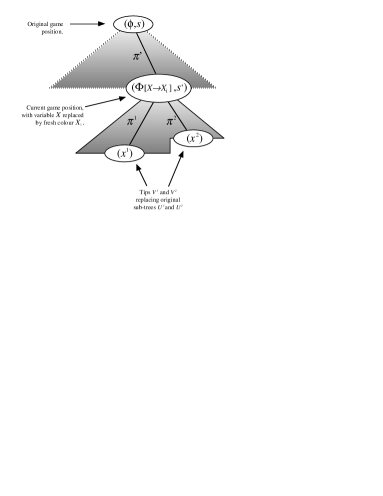
Figure 7: Left-hand side of (18): tree $T$ after subtrees $U^{k}$ replaced by tips $V^{k}$.

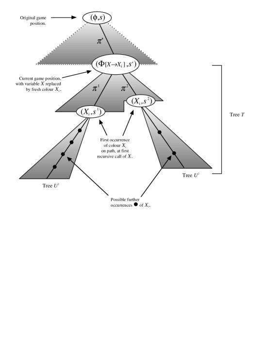
Figure 8: Right-hand side of (18): tree $T$ before subtrees $U^{k}$ replaced by tips $V^{k}$.

We will now show that the left-hand side of (18) is equal to $[{\dagger}]$. The tree used there (Fig. 7) is

$$T[\langle\pi^{0},U^{0}\rangle\mapsto V^{0},\langle\pi^{1},U^{1}\rangle\mapsto V^{1}\cdots]~{},$$

— i.e. the result of all the $k$-indexed substutitions done simultaneously — and each $V^{k}$ is just the tip $(x^{k})$. But the tree $[\![\Phi]\!]_{{\cal V}_{[X\mapsto g]}}^{{\underline{\sigma}},{\overline{\sigma}}}.\pi^{\prime}.s^{\prime}$ used in $[{\dagger}]$ is the same except that it contains the tip $(g.\pi^{k}.s^{k})$ at those places. (The places agree because they are both determined by the occurrences of $X$ in the original formula $\Phi$.)

Comparison of the definition of $g$ (at $[{\dagger}]$) — noting its arguments at each $k$ will be $\pi^{\prime\prime}\mathrel{\hat{=}}\pi^{\prime}\mathop{{+}\!\!\!{+}}\pi^{k}$ and $s^{\prime\prime}\mathrel{\hat{=}}s^{k}$ — and the definition of $x^{k}$ (at (20)) shows those tip-values to be equal.

That concludes our justification of the final step above, and of our inductive proof of (17) as a whole.

Using (17) we finish off the proof of this case as follows. Choose path $\pi^{+}$ itself and state $s$; then with bounded monotone convergence we have

	$\begin{array}[t]{ll}(\sqcup n\mathrel{\mbox{\boldmath$\cdot$}}f^{n}.\underline{0}).\pi^{+}.s\end{array}$
$=$	$\begin{array}[t]{ll}(\sqcup n\mathrel{\mbox{\boldmath$\cdot$}}\int_{\makebox[0.0pt][l]{\raisebox{-3.61664pt}{\scriptsize$[\![\Phi_{[X\mapsto X_{i}]}]\!]_{{\cal V}}^{{\underline{\sigma}},{\overline{\sigma}}}.\pi^{+}.s$}}}~{}\textit{Val}^{\,X_{i}}_{n})\end{array}$ from (17) in the special case $\pi^{\prime}=\pi^{+}$
$=$	$\begin{array}[t]{ll}\int_{\makebox[0.0pt][l]{\raisebox{-6.02777pt}{\scriptsize$[\![\Phi_{[X\mapsto X_{i}]}]\!]_{{\cal V}}^{{\underline{\sigma}},{\overline{\sigma}}}.\pi^{+}.s$}}}~{}(\sqcup n\mathrel{\mbox{\boldmath$\cdot$}}\textit{Val}^{\,X_{i}}_{n})\end{array}$ bounded monotone convergence $(\ast)$
$=$	$\begin{array}[t]{ll}\int_{\makebox[0.0pt][l]{\raisebox{-3.61664pt}{\scriptsize$[\![\Phi_{[X\mapsto X_{i}]}]\!]_{{\cal V}}^{{\underline{\sigma}},{\overline{\sigma}}}.\pi^{+}.s$}}}~{}\textit{Val}\end{array}$ $(\sqcup n\mathrel{\mbox{\boldmath$\cdot$}}\textit{Val}^{\,X_{i}}_{n})=\textit{Val}$
$=$	$\begin{array}[t]{ll}\int_{\makebox[0.0pt][l]{\raisebox{-3.61664pt}{\scriptsize$[\![\phi]\!]_{{\cal V}}^{{\underline{\sigma}},{\overline{\sigma}}}.\pi.s$}}}~{}\textit{Val}~{}.\end{array}$ tree-building step for $\mu$ (backwards); $X_{i}$ looks up $\Phi_{[X\mapsto X_{i}]}$ in $\pi^{+}$

where the final step is the one in which colour $X_{i}$ was generated.

Inductive case $\phi$ is $(\nu X\mathrel{\mbox{\boldmath$\cdot$}}\Phi)$

— This case is essentially the same as the $\mu$-case — we define the truncated valuations $\textit{Val}^{\,X_{i}}_{n}.\pi^{\prime}$ as before except that paths $\pi^{\prime}$ with at least $n$ occurrences of $X_{i}$ are taken to one (rather than to zero).

A small complication however occurs in the use of bounded monotone convergence, which requires the sequence of valuations to be monotone non-decreasing: at the point corresponding to $(\ast)$ above we would in this case be arguing that

$$(\sqcap n\mathrel{\mbox{\boldmath$\cdot$}}\int_{\makebox[0.0pt][l]{\raisebox{-3.61664pt}{\scriptsize$[\![\Phi_{[X\mapsto X_{i}]}]\!]_{{\cal V}}^{{\underline{\sigma}},{\overline{\sigma}}}.\pi^{+}.s$}}}~{}\textit{Val}^{\,X_{i}}_{n})~{}~{}~{}~{}~{}~{}~{}~{}~{}\quad=~{}~{}~{}~{}~{}~{}~{}~{}~{}\int_{\makebox[0.0pt][l]{\raisebox{-6.02777pt}{\scriptsize$[\![\Phi_{[X\mapsto X_{i}]}]\!]_{{\cal V}}^{{\underline{\sigma}},{\overline{\sigma}}}.\pi^{+}.s$}}}~{}(\sqcap n\mathrel{\mbox{\boldmath$\cdot$}}\textit{Val}^{\,X_{i}}_{n})~{},$$

where the terms are non-increasing. Since all the terms lie in $[0,1]$ however, we can deal with it by subtracting from one throughout, before and after.

Appendix 0.B Memoriless strategies suffice over a finite state space

We show that for any formula $\phi$, possibly including $\sqcap$ and $\sqcup$ strategy operators, there are specific state predicates (collected into tuples $\underline{\sf G}$ and $\overline{\sf G}$) that can replace the strategy operators without affecting the value of the formula. The inductive proof is straightforward except for replacement of $\sqcup$ within $\mu$ (and, dually, replacement of $\sqcap$ within $\nu$). For this $\overline{\sf G}$/$\mu$ case we need several technical lemmas and definitions; the other cases are set out at [28].

Because the argument in this section is mainly over properties of real-valued functions, we shift to a more mathematical style of presentation. Variables $f,g,\ldots$ denote (Curried) functions of type expectation(s) to expectation, and $w,x,\ldots$ are expectations in ${\cal E}S$. For function $f$ of one argument we write $\mu.f$ for its least fixed-point.

Definition 3

Almost-linear —  Say that an expectation-valued function $f$ of possibly several expectation arguments $x,y,\cdots,z$ is almost-linear if it can be written in the form

$$f.x.y\cdots.z~{}~{}~{}\mathrel{\hat{=}}~{}~{}~{}w+g.x+h.y+\cdots+i.z~{},$$ (21)

where $w$ is an expectation and $g,h,\cdots,i$ are linear expectation-valued functions of their single arguments.

Lemma 7

Every $\sqcap$/$\sqcup$-free formula $\phi$, possibly containing free expectation variables $X,Y,\ldots,Z$, denotes an almost-linear function of the values assigned to those arguments.

Proof

(sketch) What we are claiming is that the function

$$f.x.y\cdots.z~{}~{}~{}\mathrel{\hat{=}}~{}~{}~{}|\!|\phi|\!|_{{\cal V}[x,y\cdots z/X,Y\cdots Z]}$$

can be written in the form given on the right at (21), provided $\phi$ contains no $\sqcap$ or $\sqcup$. This is a straightforward structural induction over $\phi$, given in full at [28].

Definition 4

Almost less-than —  For non-negative reals $a,b$, write $a\ll b$ for $a>0\mathrel{\Rightarrow}a<b$; write the same for the pointwise-extended relation over expectations. Note that $a<b$ implies $a\ll b$ implies $a\leq b$ on this domain.

Definition 5

ok functions —  Say that an expectation-to-expectation function $f$ of one argument is ok if for all expectations $x$ with $x\ll f.x$ we have that $x\leq\mu.f$  .

Lemma 8

If $f$ is almost-linear then $f$ is ok in each argument separately.

Proof

See Appendix 0.D.

Lemma 9

All $\sqcap$/$\sqcup$-free formulae $\phi$ denote ok functions of their free expectations $X,Y,\cdots,Z$ taken separately.

Proof

Lemmas 7 and 8.

The following result forms the core of Everett’s argument [10]; note it does not depend on $f$’s being ok.

Lemma 10

For any monotonic and continuous function $f$ over expectations, and any $\varepsilon>0$, there is an expectation $x$ such that

$$x \ll f.x$$ (22)

$$\textrm{and\hskip 50.00008pt}\mathop{\sf lfp}.f-\underline{\varepsilon} \leq x~{},$$ (23)

where $\underline{\varepsilon}$ is the everywhere-$\varepsilon$ expectation. That is, we can find an almost-increased-by-$f$ expectation $x$ that approaches $\mathop{\sf lfp}.f$ as closely as we please from below.

Proof

Define a subset $T$ of the state space $S$ by

$$T~{}~{}~{}\mathrel{\hat{=}}~{}~{}~{}\{s\colon S\mid f.\underline{0}.s=\mathop{\sf lfp}.f.s\}~{},$$ (24)

so that the subset $T$ is “the termination set for $f$,” comprising those states at which $f$ reaches its fixed-point in just one step. Because $S$ is finite we can proceed by induction decreasing over these sets $T$ determined by $f$, with the base case therefore being when $T$ is all of $S$.

We strengthen Condition (23) of the inductive hypothesis to read

$\mathop{\sf lfp}.f-\underline{\varepsilon}~{}~{}~{}\leq~{}~{}~{}x~{}~{}~{}\leq~{}~{}~{}\mathop{\sf lfp}.f$ . (23a)

Case $T=S$

— Define $x\mathrel{\hat{=}}(\mathop{\sf lfp}.f-\underline{\varepsilon})\sqcup\underline{0}$ so that (23a) is satisfied trivially. Since $\varepsilon>0$ we have also that $x\ll\mathop{\sf lfp}.f$, and then from $T=S$ and monotonicity of $f$ we reason

$$x~{}~{}~{}\ll~{}~{}~{}\mathop{\sf lfp}.f~{}~{}~{}=~{}~{}~{}f.\underline{0}~{}~{}~{}\leq~{}~{}~{}f.x~{},$$

sufficient for (22).

Case $T\subset S$

— Pick $s^{\ast}$ from $S-T$, and for all $x$ define

$$f^{\ast}_{v}.x~{}~{}~{}\mathrel{\hat{=}}~{}~{}~{}f.x_{[s^{\ast}\mapsto v]}~{},$$

that is the expectation that agrees with $f.x$ everywhere except possibly at $s^{\ast}$ where it takes the value $v$ instead. Define also $v^{\ast}\mathrel{\hat{=}}\mathop{\sf lfp}.f.s^{\ast}$, and note that $v^{\ast}>0$ because otherwise we would have $s^{\ast}\in T$.

We begin by showing two things about $f^{\ast}_{v}$. The first (a) is that “the termination set for $f^{\ast}_{v}$” — that is $T^{\ast}_{v}\mathrel{\hat{=}}\{s\colon S\mid f^{\ast}_{v}.\underline{0}.s=\mathop{\sf lfp}.f^{\ast}_{v}.s\}$ — is a strict superset of $T$ when $v\leq v^{\ast}$, which will allow an appeal to the inductive hypothesis. The second (b) is that the function $\mathop{\sf lfp}.f^{\ast}_{v}$ of $v$ approaches $\mathop{\sf lfp}.f$ as $v$ approaches $v^{\ast}$ from below, and attains it in the limit.

To show (a) we assume $v\leq v^{\ast}$ and note first that

$$\mathop{\sf lfp}.f^{\ast}_{v}~{}~{}~{}\leq~{}~{}~{}\mathop{\sf lfp}.f~{},$$ (25)

because

$$\begin{array}[]{r@{\quad}ccccc@{\quad}l}&f^{\ast}_{v}.(\mathop{\sf lfp}.f).s&~{}~{}~{}={}{}{}&f.(\mathop{\sf lfp}.f).s&~{}~{}~{}={}{}{}&\mathop{\sf lfp}.f.s&\textrm{for $s\neq s^{\ast}$}\\ \textrm{and}&f^{\ast}_{v}.(\mathop{\sf lfp}.f).s^{\ast}&~{}~{}~{}={}{}{}&v&~{}~{}~{}\leq{}{}{}&\mathop{\sf lfp}.f.s^{\ast}&\textrm{by assumption.}\end{array}$$

That establishes $f^{\ast}_{v}.(\mathop{\sf lfp}.f)\leq\mathop{\sf lfp}.f$, sufficient for (25) by the least-fixed-point property.

From (25) we show $T\cup\{s^{\ast}\}\subseteq T^{\ast}_{v}$ by considering two cases:

Case $s\in T$:

We have

	$\begin{array}[t]{ll}f^{\ast}_{v}.\underline{0}.s\end{array}$
$\leq$	$\begin{array}[t]{ll}f^{\ast}_{v}.(\mathop{\sf lfp}.f^{\ast}_{v}).s\end{array}$ monotonicity
$=$	$\begin{array}[t]{ll}\mathop{\sf lfp}.f^{\ast}_{v}.s\end{array}$ fixed point
$\leq$	$\begin{array}[t]{ll}\mathop{\sf lfp}.f.s\end{array}$ (25)
$=$	$\begin{array}[t]{ll}f.\underline{0}.s\end{array}$ $s\in T$
$=$	$\begin{array}[t]{ll}f^{\ast}_{v}.\underline{0}.s~{}.\end{array}$ $s\neq s^{\ast}$

Case $s=s^{\ast}$:

We have

	$\begin{array}[t]{ll}f^{\ast}_{v}.\underline{0}.s^{\ast}\end{array}$
$=$	$\begin{array}[t]{ll}v\end{array}$ definition $f^{\ast}_{v}$
$=$	$\begin{array}[t]{ll}f^{\ast}_{v}.(\mathop{\sf lfp}.f^{\ast}_{v}).s^{\ast}\end{array}$ again definition $f^{\ast}_{v}$
$=$	$\begin{array}[t]{ll}\mathop{\sf lfp}.f^{\ast}_{v}.s^{\ast}~{}.\end{array}$ fixed point

Thus when $v\leq v^{\ast}$ we have $T\subset T\cup\{s^{\ast}\}\subseteq T^{\ast}_{v}$, which establishes (a).

To show (b) we note first that $\mathop{\sf lfp}.f^{\ast}_{v}$ is a continuous function of $v$ as $v$ increases. Thus we need only demonstrate that $\mathop{\sf lfp}.f^{\ast}_{v^{\ast}}=\mathop{\sf lfp}.f$, since (25) already shows that $\mathop{\sf lfp}.f^{\ast}_{v}$ is below $\mathop{\sf lfp}.f$ for $v\leq v^{\ast}$. Again we consider two cases (and appeal to (25) itself in the second case):

Case $s\neq s^{\ast}$:

We have $f.(\mathop{\sf lfp}.f^{\ast}_{v^{\ast}}).s~{}=~{}f^{\ast}_{v^{\ast}}.(\mathop{\sf lfp}.f^{\ast}_{v^{\ast}}).s~{}=~{}\mathop{\sf lfp}.f^{\ast}_{v^{\ast}}.s$ .

Case $s=s^{\ast}$:

We have

	$\begin{array}[t]{ll}f.(\mathop{\sf lfp}.f^{\ast}_{v^{\ast}}).s^{\ast}\end{array}$
$\leq$	$\begin{array}[t]{ll}f.(\mathop{\sf lfp}.f).s^{\ast}\end{array}$ by (25) in the special case $v=v^{\ast}$
$=$	$\begin{array}[t]{ll}\mathop{\sf lfp}.f.s^{\ast}\end{array}$ fixed point
$=$	$\begin{array}[t]{ll}v^{\ast}\end{array}$ definition $v^{\ast}$
$=$	$\begin{array}[t]{ll}f^{\ast}_{v^{\ast}}.(\mathop{\sf lfp}.f^{\ast}_{v^{\ast}}).s^{\ast}\end{array}$ definition $f^{\ast}_{v^{\ast}}$
$=$	$\begin{array}[t]{ll}\mathop{\sf lfp}.f^{\ast}_{v^{\ast}}.s^{\ast}~{}.\end{array}$ fixed point

Thus $f.(\mathop{\sf lfp}.f^{\ast}_{v^{\ast}})\leq\mathop{\sf lfp}.f^{\ast}_{v^{\ast}}$, whence by the least-fixed-point property we have $\mathop{\sf lfp}.f\leq\mathop{\sf lfp}.(f^{\ast}_{v^{\ast}})$ which — with (25) again in the case $v=v^{\ast}$ — gives the equality we need and establishes (b).

With (a) and (b) secure, we proceed to the main proof: we make a particular choice of $v$ and appeal to the induction hypothesis in respect of $f^{\ast}_{v}$ to find an expectation close to $\mathop{\sf lfp}.f^{\ast}_{v}$, and we then show how to derive from that a suitable expectation $x$ satisfying (22,23a) as required for the function $f$ in this case.

We choose $v$ first. From (b) we can choose $v<v^{\ast}$ to achieve

$$\mathop{\sf lfp}.f-\underline{\varepsilon_{1}}~{}~{}~{}\leq~{}~{}~{}\mathop{\sf lfp}.f^{\ast}_{v}~{}~{}~{}\leq~{}~{}~{}\mathop{\sf lfp}.f$$ (26)

for any $\varepsilon_{1}<\varepsilon$ we please.

Now we appeal to the induction hypothesis: since $T\subset T^{\ast}_{v}$, for any $0<\varepsilon_{2}\leq\varepsilon-\varepsilon_{1}$ we can find an $x^{\varepsilon_{2}}_{v}$ satisfying

$$\mathop{\sf lfp}.f^{\ast}_{v}-\underline{\varepsilon_{2}} ~{}~{}~{}\leq~{}~{}~{} x^{\varepsilon_{2}}_{v}~{}~{}~{}\leq~{}~{}~{}\mathop{\sf lfp}.f^{\ast}_{v}$$ (27)

$$\textrm{and\hskip 50.00008pt}x^{\varepsilon_{2}}_{v} ~{}~{}~{}\ll~{}~{}~{} f^{\ast}_{v}.x^{\varepsilon_{2}}_{v}~{}.$$ (28)

From that we have immediately

	$\begin{array}[t]{ll}\mathop{\sf lfp}.f-\underline{\varepsilon}\end{array}$
$\leq$	$\begin{array}[t]{ll}\mathop{\sf lfp}.f-\underline{\varepsilon_{1}}-\underline{\varepsilon_{2}}\end{array}$ choice of $\varepsilon_{2}$
$\leq$	$\begin{array}[t]{ll}\mathop{\sf lfp}.f^{\ast}_{v}-\varepsilon_{2}\end{array}$ left-hand inequality at (26)
$\leq$	$\begin{array}[t]{ll}x^{\varepsilon_{2}}_{v}\end{array}$ left-hand inequality at (27)
$\leq$	$\begin{array}[t]{ll}\mathop{\sf lfp}.f^{\ast}_{v}\end{array}$ right-hand inequality at (27)
$\leq$	$\begin{array}[t]{ll}\mathop{\sf lfp}.f~{},\end{array}$ left-hand inequality at (26)

which is our (23a) if we take $x$ to be $x^{\varepsilon_{2}}_{v}$.

All that remains is (22), for which we require $x^{\varepsilon_{2}}_{v}\ll f.x^{\varepsilon_{2}}_{v}$ — and indeed that holds trivially everywhere except possibly at $s^{\ast}$: for if $s\neq s^{\ast}$ we have from (28) that

$$x^{\varepsilon_{2}}_{v}.s~{}~{}~{}\ll~{}~{}~{}f^{\ast}_{v}.x^{\varepsilon_{2}}_{v}.s~{}~{}~{}=~{}~{}~{}f.x^{\varepsilon_{2}}_{v}.s~{}.$$ (29)

Thus all we are left with is to show that $x^{\varepsilon_{2}}_{v}.s^{\ast}~{}\ll~{}f.x^{\varepsilon_{2}}_{v}.s^{\ast}$, which unfortunately is not true for all $x^{\varepsilon_{2}}_{v}$ satisfying (27,28). But, as we demonstrate in the technical Lem. 12 proved in App. 0.C below, for any $\varepsilon_{2}>0$ it is possible to find an $\varepsilon^{\ast}_{2}$ with $0<\varepsilon^{\ast}_{2}\leq\varepsilon_{2}$ which retains the properties (27,28,29) above and satisfies $x^{\varepsilon^{\ast}_{2}}_{v}.s^{\ast}~{}\ll~{}f.x^{\varepsilon^{\ast}_{2}}_{v}.s^{\ast}$ as well — and which thus completes the proof.

We can now sketch the proof of the main result of this section.

Lemma 11

Fixed strategies suffice —  For any formula $\phi$, possibly containing strategy operators $\sqcap$/$\sqcup$, and valuation ${\cal V}$, there are state-predicate tuples $\underline{\sf G}$/$\overline{\sf G}$ — possibly depending on ${\cal V}$ — such that

$$|\!|\phi_{\underline{\sf G}}|\!|_{{\cal V}}~{}~{}~{}=~{}~{}~{}|\!|\phi|\!|_{{\cal V}}~{}~{}~{}=~{}~{}~{}|\!|\phi_{\overline{\sf G}}|\!|_{{\cal V}}~{}.$$

Proof

(sketch) We give only the $\mu$-case of an otherwise straightforward induction over the size of $\phi$; a full proof may be found at [28].

Suppose we are considering the case where $\phi$ is a least-fixed-point $(\mu X\mathrel{\mbox{\boldmath$\cdot$}}\Phi)$. Let $f$ be the function denoted by $\Phi$ with respect to a single expectation-valued argument $x$ supplied for the variable $X$, with the values of any other free variables in $\Phi$ fixed by the environment ${\cal V}$; for any $\underline{\sf G},\overline{\sf G}$ let functions $f_{\overline{\sf G}}$ and $f_{\underline{\sf G},\overline{\sf G}}$ be derived similarly from $\Phi_{\overline{\sf G}}$ and $\Phi_{\underline{\sf G},\overline{\sf G}}$.

Case $\underline{\sf G}$

— We must show $\mu.f=\mu.f_{\underline{\sf G}}$ for some $\underline{\sf G}$; note that $\mu.f\leq\mu.f_{\underline{\sf G}}$ trivially, since $f\leq f_{\underline{\sf G}}$. Since $\Phi$ is smaller in size than $\phi$, our inductive hypothesis provides for any $x$ a $\underline{\sf G}_{x}$ so that $f_{\underline{\sf G}_{x}}.x=f.x$; take $x=\mu.f$ and therefore choose $\underline{\sf G}$ so that $f_{\underline{\sf G}}.(\mu.f)=f.(\mu.f)=\mu.f$. Thus $\mu.f$ is a fixed-point of $f_{\underline{\sf G}}$, whence immediately $\mu.f_{\underline{\sf G}}\leq\mu.f$.

Case $\overline{\sf G}$

— In this case must show $\mu.f=\mu.f_{\overline{\sf G}}$ for some $\overline{\sf G}$; again it is trivial that $\mu.f_{\overline{\sf G}}\leq\mu.f$ for any $\overline{\sf G}$.

For the other direction, in fact we show that for any $\varepsilon>0$ there is a $\overline{\sf G}_{\varepsilon}$ such that $\mu.f_{\overline{\sf G}_{\varepsilon}}\geq\mu.f-\varepsilon$ — whence the existence of a single $\overline{\sf G}$ satisfying $\mu.f_{\overline{\sf G}}\geq\mu.f$ follows from the finiteness of the state space (since the set of possible strategy tuples for this $f$ is therefore finite as well, and so there must be one that works for all $\varepsilon$).

$+$       Because we know inductively that $f$ is a minimax over strategy tuples $\underline{\sf G}^{\prime},\overline{\sf G}^{\prime}$ of almost-linear functions $f_{\underline{\sf G}^{\prime},\overline{\sf G}^{\prime}}$, that those functions are continuous by construction, and that the minimax is finite because there are only finitely many strategy tuples $\underline{\sf G}^{\prime},\overline{\sf G}^{\prime}$ for this $f$, we know that $f$ is continuous itself, and by Lem. 10 we therefore have an expectation $x_{\varepsilon}$ with

$$\mu.f-\varepsilon\leq x_{\varepsilon}\quad\quad\textrm{and}\quad\quad x_{\varepsilon}\ll f.x_{\varepsilon}~{}.$$ (30)

To get our result we need only show in addition that $x_{\varepsilon}\leq\mu.f_{\overline{\sf G}_{\varepsilon}}$ for some $\overline{\sf G}_{\varepsilon}$.

From our inductive hypothesis we can choose $\overline{\sf G}_{\varepsilon}$ so that $f.x_{\varepsilon}=f_{\overline{\sf G}_{\varepsilon}}.x_{\varepsilon}$, whence from (30) we have $x_{\varepsilon}\ll f_{\overline{\sf G}_{\varepsilon}}.x_{\varepsilon}$. But in fact $f_{\overline{\sf G}_{\varepsilon}}$ is ok (see below), so from Def. 5 we have $x_{\varepsilon}\leq\mu.f_{\overline{\sf G}_{\varepsilon}}$ and we are done.

 

To see that $f_{\overline{\sf G}_{\varepsilon}}$ is ok, we apply the argument of Case $\underline{\sf G}$, which gives us a $\underline{\sf G}^{\prime}$ with $\mu.f_{\overline{\sf G}_{\varepsilon}}=\mu.f_{\underline{\sf G}^{\prime},\overline{\sf G}_{\varepsilon}}$. Now consider any $x$ such that $x\ll f_{\overline{\sf G}_{\varepsilon}}.x$ .

Since $f_{\overline{\sf G}_{\varepsilon}}.x\leq f_{\underline{\sf G}^{\prime},\overline{\sf G}_{\varepsilon}}.x$ we have $x\ll f_{\underline{\sf G}^{\prime},\overline{\sf G}_{\varepsilon}}.x$ also — but we recall from Lem. 9 that $f_{\underline{\sf G}^{\prime},\overline{\sf G}_{\varepsilon}}$ is ok. Hence $x\leq\mu.f_{\underline{\sf G}^{\prime},\overline{\sf G}_{\varepsilon}}=\mu.f_{\overline{\sf G}_{\varepsilon}}$ , and $f_{\overline{\sf G}_{\varepsilon}}$ is ok as well.

Appendix 0.C A technical lemma used in App. 0.B

Lemma 12

In this technical lemma we continue the notation established within the proof of Lem. 10; we show that for any $\varepsilon_{2}>0$ there is an $\varepsilon^{\ast}_{2}$ with $0<\varepsilon^{\ast}_{2}\leq\varepsilon_{2}$ and an $x^{\varepsilon^{\ast}_{2}}_{v}$ that together retain the properties (27,28,29) and in addition satisfy $x^{\varepsilon^{\ast}_{2}}_{v}.s^{\ast}~{}\ll~{}f.x^{\varepsilon^{\ast}_{2}}_{v}.s^{\ast}$, as we require above.

Proof

In fact we find $\varepsilon^{\ast}_{2}$ and $x^{\varepsilon^{\ast}_{2}}_{v}$ which together satisfy the stronger property $x^{\varepsilon^{\ast}_{2}}_{v}.s^{\ast}~{}<~{}f.x^{\varepsilon^{\ast}_{2}}_{v}.s^{\ast}$.

Suppose for a contradiction that, for all $\varepsilon^{\prime}_{2}\leq\varepsilon_{2}$, every $x^{\varepsilon^{\prime}_{2}}_{v}$ we could choose satisfying Properties (27, 28) for $f^{\ast}_{v}$, that is $\mathop{\sf lfp}.f^{\ast}_{v}-\underline{\varepsilon^{\prime}_{2}}\leq x^{\varepsilon^{\prime}_{2}}_{v}\leq\mathop{\sf lfp}.f^{\ast}_{v}$ and $x^{\varepsilon^{\prime}_{2}}_{v}\ll f^{\ast}_{v}.x^{\varepsilon^{\prime}_{2}}_{v}$, satisfied the inequality

$$f.x^{\varepsilon^{\prime}_{2}}_{v}.s^{\ast}~{}~{}~{}\leq~{}~{}~{}x^{\varepsilon^{\prime}_{2}}_{v}.s^{\ast}$$ (31)

as well — thus failing to have the property (28) for $f$ at $s^{\ast}$ that we needed to complete our proof of Lem. 10. As $\varepsilon^{\prime}_{2}$ approaches zero we would then have from above that we can choose a sequence of $x^{\varepsilon^{\prime}_{2}}_{v}$’s approaching $\mathop{\sf lfp}.f^{\ast}_{v}$ — and so from the continuity of $f$ we could take limits on both sides of (31), giving $f.(\mathop{\sf lfp}.f^{\ast}_{v}).s^{\ast}\leq\mathop{\sf lfp}.f^{\ast}_{v}.s^{\ast}$, and so we would have

$$F.v~{}~{}~{}=~{}~{}~{}f.(\mathop{\sf lfp}.f^{\ast}_{v}).s^{\ast}~{}~{}~{}\leq~{}~{}~{}\mathop{\sf lfp}.f^{\ast}_{v}.s^{\ast}~{}~{}~{}=~{}~{}~{}v~{},$$ (32)

where on the left we are defining a function $F$ of $v$ for use below — our contradiction will be achieved by considering a further property of $F$, beyond the $F.v\leq v$ that we have at (32) already.

That property is $v^{\ast}\leq\mathop{\sf lfp}.F$. To see that we argue by cases that

$$f.(\mathop{\sf lfp}.f^{\ast}_{\mathop{\sf lfp}.F})~{}~{}~{}=~{}~{}~{}\mathop{\sf lfp}.f^{\ast}_{\mathop{\sf lfp}.F}~{},$$

which by the least-fixed-point property gives us $\mathop{\sf lfp}.f\leq\mathop{\sf lfp}.f^{\ast}_{\mathop{\sf lfp}.F}$. Then, applying that inequality at $s^{\ast}$ itself, we have $\mathop{\sf lfp}.f.s^{\ast}\leq\mathop{\sf lfp}.f^{\ast}_{\mathop{\sf lfp}.F}.s^{\ast}$, whence

	$\begin{array}[t]{ll}v^{\ast}\end{array}$
$=$	$\begin{array}[t]{ll}\mathop{\sf lfp}.f.s^{\ast}\end{array}$ definition $v^{\ast}$
$\leq$	$\begin{array}[t]{ll}\mathop{\sf lfp}.f^{\ast}_{\mathop{\sf lfp}.F}.s^{\ast}\end{array}$ immediately above
$=$	$\begin{array}[t]{ll}f^{\ast}_{\mathop{\sf lfp}.F}.(\mathop{\sf lfp}.f^{\ast}_{\mathop{\sf lfp}.F}).s^{\ast}\end{array}$ fixed point
$=$	$\begin{array}[t]{ll}\mathop{\sf lfp}.F~{},\end{array}$ definition: $f^{\ast}_{x}.y.s^{\ast}\mathrel{\hat{=}}x$, for all $x,y$

as required. The two cases are

Case $s\neq s^{\ast}$:

We have

	$\begin{array}[t]{ll}f.(\mathop{\sf lfp}.f^{\ast}_{\mathop{\sf lfp}.F}).s\end{array}$
$=$	$\begin{array}[t]{ll}f^{\ast}_{\mathop{\sf lfp}.F}.(\mathop{\sf lfp}.f^{\ast}_{\mathop{\sf lfp}.F}).s\end{array}$ definition: $f^{\ast}_{x}.y.s\mathrel{\hat{=}}f.y.s$, for all $x,y$ and $s\neq s^{\ast}$
$=$	$\begin{array}[t]{ll}\mathop{\sf lfp}.f^{\ast}_{\mathop{\sf lfp}.F}.s~{}.\end{array}$ fixed point

Case $s=s^{\ast}$:

We have

	$\begin{array}[t]{ll}f.(\mathop{\sf lfp}.f^{\ast}_{\mathop{\sf lfp}.F}).s^{\ast}\end{array}$
$=$	$\begin{array}[t]{ll}F.(\mathop{\sf lfp}.F)\end{array}$ definition $F$
$=$	$\begin{array}[t]{ll}\mathop{\sf lfp}.F\end{array}$ fixed point
$=$	$\begin{array}[t]{ll}f^{\ast}_{\mathop{\sf lfp}.F}.(\mathop{\sf lfp}.f^{\ast}_{\mathop{\sf lfp}.F}).s^{\ast}\end{array}$ definition $f^{\ast}_{\cdot}$
$=$	$\begin{array}[t]{ll}\mathop{\sf lfp}.f^{\ast}_{\mathop{\sf lfp}.F}.s^{\ast}~{}.\end{array}$ fixed point

That establishes the equality we used above, and completes the demonstration that $v^{\ast}\leq\mathop{\sf lfp}.F$.

Now from that and $v<v^{\ast}$ we have immediately that $v<\mathop{\sf lfp}.F$ also and, since $F$ is monotonic (it is constructed from monotonic pieces), by the least-fixed-point property we have $F.v\not\leq v$ — which contradicts (32). Therefore our assumption must fail: there must be some $0<\varepsilon^{\ast}_{2}\leq\varepsilon_{2}$ for which not all choices of $x^{\varepsilon^{\ast}_{2}}_{v}$ satisfying (27) satisfy (31) as well — that is, at least one will satisfy (28) at $s^{\ast}$. That is the value we take.

Appendix 0.D Proof of Lem. 8 from App. 0.B

We prove in several stages that if $f$ is almost-linear then $f$ is ok in each argument separately, beginning with some preliminary lemmas.

Lemma 13

Almost-feasibility —  Let transformer $f$ be almost-linear, and suppose for some state $s$ that $f.0.y.\cdots.z.s=0$, where wlog we concentrate on the first argument of $f$. Then for any expectation $x$ we have $f.x.y.\cdots.z.s\leq(\sqcup s\colon S\mathrel{\mbox{\boldmath$\cdot$}}x.s)$.

Proof

This is clear from the explicit form (refer Def. 3) that almost-linear transformers take: if $f.0.y.\cdots.z.s$ is zero, then all non-$x$ terms $w.s,h.y.s,\cdots,i.z.s$ in $f$ must be zero — that is, for those values $y,\cdots,z,s$ we have $f.x.y.\cdots.z.s=g.x.s$ for some one-bounded linear transformer $g$, from which property of $g$ we have $g.x.s\leq(\sqcup s\colon S\mathrel{\mbox{\boldmath$\cdot$}}x.s)$.

From now on we will fix the non-$x$ arguments of $f$, and omit them for brevity.

Lemma 14

Stationary zeroes —  Let transformer $f$ be almost-linear, and define its kernel $K$ to be those states on which its fixed-point is zero: that is, $K\mathrel{\hat{=}}\{s\colon S\mid\mu.f.s=0\}$.

Then in effect the probabilistic game $f$ cannot escape from $K$: for any state $k$ in $K$ and expectation $x$, we have

$$f.x.k~{}~{}~{}=~{}~{}~{}f.(x{\downarrow}K).k~{},$$

where $(x{\downarrow}K).s\mathrel{\hat{=}}x.s~{}\textrm{\text@underline{if}}~{}s{\in}K~{}\textrm{\text@underline{else}}~{}0$ .

Proof

Because $\mu.f$ is non-zero everywhere outside $K$, and our state space $S$ is finite, there is an $\varepsilon>0$ so that $\varepsilon\times x{\downarrow}(S-K)~{}\leq~{}\mu.f$ whence, for $k$ in $K$, we have

$$f.(\varepsilon\times x{\downarrow}(S-K)).k~{}~{}~{}\leq~{}~{}~{}f.(\mu.f).k~{}~{}~{}=~{}~{}~{}\mu.f.k~{}~{}~{}=~{}~{}~{}0~{}.$$

From that, the almost-linearity of $f$ and that $\varepsilon>0$ we have $f.(x{\downarrow}(S-K)).k=0$. Again using almost-linearity, we continue

	$\begin{array}[t]{ll}f.x.k\end{array}$
$=$	$\begin{array}[t]{ll}f.(x{\downarrow}K+x{\downarrow}(S-K)).k\end{array}$
$\leq$	$\begin{array}[t]{ll}f.(x{\downarrow}K).k~{}~{}~{}+~{}~{}~{}f.(x{\downarrow}(S-K)).k\end{array}$ almost-linearity
$=$	$\begin{array}[t]{ll}f.(x{\downarrow}K).k~{}.\end{array}$ $f.(x{\downarrow}(S-K)).k=0$, shown above

The opposite inequality is immediate from monotonicity.

Lemma 15

Almost-linear is almost ok —  Let transformer $f$ be almost-linear, and suppose for some expectation $x$ that $x\ll f.x$ . Then for all $k$ in the kernel $K$ of $f$ we have $x.k=0$.

Proof

If $x$ is not zero on $K$ then $K$ must be non-empty and there must be a state $k^{\ast}$ in $K$ at which $x$ attains a non-zero maximum $(\sqcup k\colon K\mathrel{\mbox{\boldmath$\cdot$}}x.k)$. Then because $x\ll f.x$ we have $x.k^{\ast}<f.x.k^{\ast}=f.(x{\downarrow}K).k^{\ast}$ from Lem. 14.

Now $f.0.k^{\ast}\leq f.(\mu.f).k^{\ast}=\mu.f.k^{\ast}=0$, since $k^{\ast}\in K$,so that from Lem. 13 we have as well that $f.(x{\downarrow}K).k^{\ast}\leq(\sqcup k\colon K\mathrel{\mbox{\boldmath$\cdot$}}x.k)$ . Taken together with the above, that gives $x.k^{\ast}<(\sqcup k\colon K\mathrel{\mbox{\boldmath$\cdot$}}x.k)$, contradicting the choice of $k^{\ast}$.

We can now proceed with the proof of Lem. 8; we assume $x\ll f.x$.

First choose a real scalar $\varepsilon>0$ so that

$$\frac{\mu.f.s}{x.s}~{}~{}~{}\geq~{}~{}~{}\frac{\varepsilon}{\varepsilon+1}\quad\textrm{for all $s$ with $x.s\neq 0$,}$$

which is possible because $S$ is finite, and note that $(\varepsilon+1)(\mu.f)-\varepsilon x\geq 0$ then holds for all states — since when $\mu.f.s=0$ we have from Lem. 15 that $x.s=0$ as well. In fact we can decrease $\varepsilon$ still further, if necessary, to achieve

$$0~{}~{}~{}\leq~{}~{}~{}(\varepsilon+1)(\mu.f)-\varepsilon x~{}~{}~{}\leq~{}~{}~{}1~{},$$

sufficient to use the expression as a one-bounded expectation in the argument below.

Now because $f$ is almost-linear, as a function of $x$ it is of the form $w+g.x$ for fixed expectation $w$ and linear $g$. Applying $f$ to our expression above, and using linearity of $g$, we have

	$\begin{array}[t]{ll}f.(~{}(\varepsilon+1)\mu.f~{}-~{}\varepsilon x~{})\end{array}$
$=$	$\begin{array}[t]{ll}w~{}~{}~{}+~{}~{}~{}g.(~{}(\varepsilon+1)\mu.f~{}-~{}\varepsilon x~{})\end{array}$
$=$	$\begin{array}[t]{ll}w~{}~{}~{}+~{}~{}~{}g.(~{}(\varepsilon+1)\mu.f~{})~{}~{}~{}-~{}~{}~{}g.(\varepsilon x)\end{array}$ $g$ linear
$=$	$\begin{array}[t]{ll}w~{}~{}~{}+~{}~{}~{}(\varepsilon+1)(g.(\mu.f))~{}~{}~{}-~{}~{}~{}\varepsilon(g.x)\end{array}$
$=$	$\begin{array}[t]{ll}(\varepsilon+1)w~{}+~{}(\varepsilon+1)(g.(\mu.f))~{}~{}~{}-~{}~{}~{}\varepsilon w~{}-~{}\varepsilon(g.x)\end{array}$
$=$	$\begin{array}[t]{ll}(\varepsilon+1)(f.(\mu.f))~{}~{}~{}-~{}~{}~{}\varepsilon(f.x)\end{array}$
$\leq$	$\begin{array}[t]{ll}(\varepsilon+1)(\mu.f)~{}~{}~{}-~{}~{}~{}\varepsilon x~{},\end{array}$ $x\leq f.x$, because $x\ll f.x$

so showing that $(\varepsilon+1)(\mu.f)-\varepsilon x$ is a pre-least-fixed-point of $f$.

Thus by the least-fixed-point property we have

$$\mu.f~{}~{}~{}\leq~{}~{}~{}(\varepsilon+1)(\mu.f)~{}-~{}\varepsilon x~{},$$

whence by arithmetic (rearranging, dividing by $\varepsilon>0$) we have $x\leq\mu.f$ .

Thus we have proved that all almost-linear transformers are ok.

References

- [1] A. Aziz, V. Singhal, F. Balarinand R.K. Brayton, and A.L. Sangiovanni-Vincentelli. It usually works: The temporal logic of stochastic systems. In Computer-Aided Verification, 7th Intl. Workshop, volume 939 of LNCS. Springer Verlag, 1995.
- [2] M. Ben-Ari, A. Pnueli, and Z. Manna. The temporal logic of branching time. Acta Informatica, 20:207–226, 1983.
- [3] Andrea Bianco and Luca de Alfaro. Model checking of probabilistic and nondeterministic systems. In Foundations of Software Technology and Theoretical Computer Science, volume 1026 of LNCS, pages 499–512, December 1995.
- [4] A. Condon. The complexity of stochastic games. Information and Computation, 96(2):203–224, 1992.
- [5] P. Cousot and R. Cousot. Abstract interpretation frameworks. Journal of Logic and Computation, 2(2):511–547, 1992.
- [6] Luca de Alfaro. Temporal logics for the specification of performance and reliability. In STACS ’97, volume 1200 of LNCS, 1997.
- [7] Luca de Alfaro. Computing minimum and maximum reachability times in probabilistic systems. In Proceedings of CONCUR ’99, LNCS. Springer Verlag, 1999.
- [8] Luca de Alfaro. Quantitative verification and control via the mu-calculus. In Proceedings of CONCUR ’03, LNCS. Springer Verlag, 2003.
- [9] Luca de Alfaro and Rupak Majumdar. Quantitative solution of omega-regular games. In Proc. STOC ’01, 2001.
- [10] H. Everett. Recursive games. In Contributions to the Theory of Games III, volume 39 of Ann. Math. Stud., pages 47–78. Princeton University Press, 1957.
- [11] J. Filar and O.J. Vrieze. Competitive Markov Decision Processes — Theory, Algorithms, and Applications. Springer Verlag, 1996.
- [12] G.R. Grimmett and D. Welsh. Probability: an Introduction. Oxford Science Publications, 1986.
- [13] H. Hansson and B. Jonsson. A logic for reasoning about time and probability. Formal Aspects of Computing, 6(5):512–535, 1994.
- [14] Hans Hansson and Bengt Jonsson. A logic for reasoning about time and reliability. Formal Aspects of Computing, 6:512–535, 1994.
- [15] S. Hart, M. Sharir, and A. Pnueli. Termination of probabilistic concurrent programs. ACM Transactions on Programming Languages and Systems, 5:356–380, 1983.
- [16] C.A.R. Hoare. A couple of novelties in the propositional calculus. Zeitschr. für Math. Logik und Grundlagen der Math., 31(2):173–178, 1985.
- [17] Michael Huth and Marta Kwiatkowska. Quantitative analysis and model checking. In Proceedings of 12th annual IEEE Symposium on Logic in Computer Science, 1997.
- [18] D. Kozen. Semantics of probabilistic programs. Journal of Computer and System Sciences, 22:328–350, 1981.
- [19] D. Kozen. A probabilistic PDL. In Proceedings of the 15th ACM Symposium on Theory of Computing, New York, 1983. ACM.
- [20] D. Kozen. Results on the propositional -calculus. Theoretical Computer Science, 27:333–354, 1983.
- [21] M. Kwiatkowska, G. Norman, and D. Parker. PRISM: Probabilistic symbolic model checker. In T. Field, P. Harrison, J. Bradley, and U. Harder, editors, Proc. 12th International Conference on Modelling Techniques and Tools for Computer Performance Evaluation (TOOLS ’02), volume 2324 of LNCS, pages 200–204. Springer Verlag, April 2002.
- [22] A.K. McIver and C.C. Morgan. Demonic, angelic and unbounded probabilistic choices in sequential programs. Acta Informatica, 37:329–354, 2001. Available at [38, at PPT2].
- [23] A.K McIver and C.C. Morgan. Games, probability and the quantitative -calculus qMu. In Proc. LPAR, volume 2514 of LNAI, pages 292–310. Springer Verlag, 2002.
- [24] A.K. McIver, C.C. Morgan, and J.W. Sanders. Probably Hoare? Hoare probably! In A.W. Roscoe, editor, A Classical Mind: Essays in Honour of CAR Hoare. Prentice-Hall, 1999.
- [25] Annabelle McIver and Carroll Morgan. Abstraction, Refinement and Proof for Probabilistic Systems. Springer Verlag, 2004. To appear.
- [26] David Monniaux. Abstract interpretation of probabilistic semantics. In International Static Analysis Symposium (SAS ’00), volume 1824 of LNCS. Springer Verlag, 2000.
- [27] C.C. Morgan. Proof rules for probabilistic loops. In He Jifeng, John Cooke, and Peter Wallis, editors, Proceedings of the BCS-FACS 7th Refinement Workshop, Workshops in Computing. Springer Verlag, July 1996. //www.springer.co.uk/ewic/workshops/7RW.
- [28] C.C. Morgan and A.K. McIver. Proofs for Chapter 11. Draft presentations of the full proofs can be found via entry Games02 at the web site [38].
- [29] C.C. Morgan and A.K. McIver. A probabilistic temporal calculus based on expectations. In Lindsay Groves and Steve Reeves, editors, Proc. Formal Methods Pacific ’97. Springer Verlag Singapore, July 1997. Available at [38, at PTL96].
- [30] C.C. Morgan and A.K. McIver. An expectation-based model for probabilistic temporal logic. Logic Journal of the IGPL, 7(6):779–804, 1999. Available at [38, at MM97].
- [31] C.C. Morgan and A.K. McIver. pGCL: Formal reasoning for random algorithms. South African Computer Journal, 22, March 1999. Available at [38, at pGCL].
- [32] C.C. Morgan and A.K. McIver. Cost analysis of games using program logic. In Proc. of the 8th Asia-Pacific Software Engineering Conference (APSEC 2001), December 2001. Abstract only: full text available at [38, at MDP01].
- [33] C.C. Morgan and A.K. McIver. Almost-certain eventualities and abstract probabilities in the quantitative temporal logic qTL. Theoretical Computer Science, 293(3):507–534, 2003. Available at [38, at PROB-1]; earlier version appeared in CATS ’01.
- [34] C.C. Morgan, A.K. McIver, and K. Seidel. Probabilistic predicate transformers. ACM Transactions on Programming Languages and Systems, 18(3):325–353, May 1996. Available at [38, at PPT].
- [35] N. Narasimha, R. Cleaveland, and P. Iyer. Probabilistic temporal logics via the modal mu-calculus. In Proceedings of the Foundation of Software Sciences and Computation Structures, Amsterdam, number 1578 in LNCS, pages 288–305, 1999.
-
[36]
The occam programming language.
//directory.google.com/Top/Computers/Programming/Languages/Occam. -
[37]
PRISM.
Probabilistic symbolic model checker.
//www.cs.bham.ac.uk/dxp/prism. -
[38]
PSG.
Probabilistic Systems Group: Collected reports.
//web.comlab.ox.ac.uk/oucl/research/areas/probs/bibliography.html. - [39] M.O. Rabin. The choice-coordination problem. Acta Informatica, 17(2):121–134, June 1982.
- [40] A.W. Roscoe. The Theory and Practice of Concurrency. Prentice-Hall, 1998.
-
[41]
Scripts for calculations of futures game example.
//www.cse.unsw.edu.au/carrollm/qmu. - [42] Roberto Segala. Modeling and Verification of Randomized Distributed Real-Time Systems. PhD thesis, MIT, 1995.
- [43] Colin Stirling. Local model checking games. In CONCUR ’95, volume 962 of LNCS, pages 1–11. Springer Verlag, 1995. Extended abstract.
- [44] Moshe Y. Vardi. A temporal fixpoint calculus. In Proc. 15th Ann. ACM Symp. on Principles of Programming Languages. ACM, January 1988. Extended abstract.
- [45] M.Y. Vardi. Branching vs. linear time: Final showdown. In Seventh International Conference on Tools and Analysis of Systems, Genova, number 2031 in LNCS, April 2001.
- [46] J. von Neumann and O. Morgenstern. Theory of Games and Economic Behavior. Princeton University Press, 1944.
- [47] I. Walukiewicz. Notes on the propositional mu-calculus: Completeness and related results. Technical Report BRICS NS-95-1, BRICS, Dept. Comp. Sci., University Aarhus, 1995. Available at //www.brics.aaudk/BRICS/.