Efficient Algorithms for Citation Network Analysis

Abstract

In the paper very efficient, linear in number of arcs, algorithms for determining Hummon and Doreian’s arc weights SPLC and SPNP in citation network are proposed, and some theoretical properties of these weights are presented. The nonacyclicity problem in citation networks is discussed. An approach to identify on the basis of arc weights an important small subnetwork is proposed and illustrated on the citation networks of SOM (self organizing maps) literature and US patents.
Keywords: large network, acyclic, citation network, main path, CPM path, arc weight, algorithm, self organizing maps, patent

1 Introduction

The citation network analysis started with the paper of Garfield et al. (1964) [10] in which the introduction of the notion of citation network is attributed to Gordon Allen. In this paper, on the example of Asimov’s history of DNA [1], it was shown that the analysis ”demonstrated a high degree of coincidence between an historian’s account of events and the citational relationship between these events”. An early overview of possible applications of graph theory in citation network analysis was made in 1965 by Garner [13].

The next important step was made by Hummon and Doreian (1989) [14, 15, 16]. They proposed three indices (NPPC, SPLC, SPNP) – weights of arcs that provide us with automatic way to identify the (most) important part of the citation network – the main path analysis.

In this paper we make a step further. We show how to efficiently compute the Hummon and Doreian’s weights, so that they can be used also for analysis of very large citation networks with several thousands of vertices. Besides this some theoretical properties of the Hummon and Doreian’s weights are presented.

The proposed methods are implemented in Pajek – a program, for Windows (32 bit), for analysis of large networks. It is freely available, for noncommercial use, at its homepage [4].

For basic notions of graph theory see Wilson and Watkins [18].

2 Citation Networks

In a given set of units $\mathbf{U}$ (articles, books, works, …) we introduce a $citing$ relation $R\subseteq\mathbf{U}\times\mathbf{U}$

$$uRv\equiv v\mbox{ cites }u$$

which determines a citation network $\mathbf{N}=(\mathbf{U},R)$.

In Table 1 some characteristics of real life citation networks are presented. Most of these networks were obtained from the Eugene Garfield’s collection of citation data [10, 12] produced using HistCite Software (formerly called HistComp – compiled Historiography program) [11]. All of these networks are the result of searches in the Web of Science and are used with the permission of ISI of Philadelphia, www.isinet.com. These networks in Pajek’s format are available from Pajek’s web site [19].

In Table 1: $n=|\mathbf{U}|$ is the number of vertices; $m=|R|$ is the number of arcs; $m_{0}$ is the number of loops; $n_{0}$ is the number of isolated vertices; $n_{C}$ is the size of the largest weakly connected component; $k_{C}$ is the number of nontrivial weakly connected components; $h$ is the depth of network (minimum number of levels); $\Delta_{in}$ is the maximum input degree; and $\Delta_{out}$ is the maximum output degree. The last three columns contain the numbers of strongly connected components (cyclic parts) of size 2, 3 and 4.

Table 1: Citation network characteristics

network	$n$	$m$	$m_{0}$	$n_{0}$	$n_{C}$	$k_{C}$	$h$	$\Delta_{in}$	$\Delta_{out}$	$2$	$3$	$4$
DNA	40	60	0	1	35	3	11	7	5	0	0	0
Coupling	223	657	1	5	218	1	16	19	134	0	0	0
Small world	396	1988	0	163	233	1	16	60	294	0	0	0
Small & Griffith	1059	4922	1	35	1024	1	28	89	232	2	0	0
Cocitation	1059	4929	1	35	1024	1	28	90	232	2	0	0
Scientometrics	3084	10416	1	355	2678	21	32	121	105	5	2	1
Kroto	3244	31950	1	0	3244	1	32	166	3243	6	0	0
SOM	4470	12731	2	698	3704	27	24	51	735	11	0	0
Zewail	6752	54253	1	101	6640	5	75	166	227	38	1	2
Lederberg	8843	41609	7	519	8212	35	63	135	1098	54	4	0
Desalination	8851	25751	7	1411	7143	115	27	73	137	12	0	1
US patents	3774768	16522438	1	0	3764117	3627	32	779	770	0	0	0

A citing relation is usually irreflexive, $\forall u\in\mathbf{U}:\lnot uRu$, and (almost) acyclic – no vertex is reachable from itself by a nontrivial path, or formally $\forall u\in\mathbf{U}\forall k\in\hbox{\sf I\kern-1.30005pt\hbox{N}}^{+}:\lnot uR^{k}u$. In the following we shall assume that it has this property. We shall postpone the question how to deal with nonacyclic citation networks till the end of the theoretical part of the paper.

For a relation $Q\subseteq\mathbf{U}\times\mathbf{U}$ we denote by $Q^{\mathrm{inv}}$ its inverse relation, $uQ^{\mathrm{inv}}v\equiv vQu$, and by

$$Q(u)=\{v\in\mathbf{U}:uQv\}$$

the set of successors of unit $u\in\mathbf{U}$. If $Q$ is acyclic then also $Q^{\mathrm{inv}}$ is acyclic. This means that the network $\mathbf{N}^{\mathrm{inv}}=(\mathbf{U},R^{\mathrm{inv}})$, $uR^{\mathrm{inv}}v\equiv u\mbox{ cites }v$, is a network of the same type as the original citation network $\mathbf{N}=(\mathbf{U},R)$. Therefore it is just a matter of ’taste’ which relation to select.

Let $I=\{(u,u):u\in\mathbf{U}\}$ be the identity relation on $\mathbf{U}$ and $\overline{Q}=\bigcup_{k\in\hbox{\sf I\kern-0.91003pt\hbox{N}}^{+}}Q^{k}$ the transitive closure of relation $Q$. Then $Q$ is acyclic iff $\overline{Q}\cap I=\emptyset$. The relation ${Q}^{\star}=\overline{Q}\cup I$ is the transitive and reflexive closure of relation $Q$.

Since the set of units $\mathbf{U}$ is finite and $R$ is acyclic we know from the theory of relations that:

• The set of units $\mathbf{U}$ can be topologically ordered – there exists a surjective mapping (permutation) $i:\mathbf{U}\to 1..|\mathbf{U}|$ with the property

  $$uRv\Rightarrow i(u)<i(v)$$

• Let $\mathop{\rm Min}\nolimits R=\{u\in\mathbf{U}:R^{\mathrm{inv}}(u)=\emptyset\}$ be the set of minimal elements and $\mathop{\rm Max}\nolimits R=\{u\in\mathbf{U}:R(u)=\emptyset\}$ the set of maximal elements. Then $\mathop{\rm Min}\nolimits R\neq\emptyset$ and $\mathop{\rm Max}\nolimits R\neq\emptyset$.

• Every unit $u\in\mathbf{U}$ and every arc $(u,v)\in R$ belong to at least one path from $\mathop{\rm Min}\nolimits R$ to $\mathop{\rm Max}\nolimits R$:
  $\forall u\in\mathbf{U}:R^{\star}(u)\cap\mathop{\rm Max}\nolimits R\neq\emptyset$
  $\forall u\in\mathbf{U}:{R^{\mathrm{inv}}}^{\star}(u)\cap\mathop{\rm Min}\nolimits R\neq\emptyset$

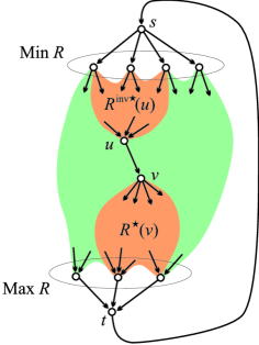
Figure 1: Citation Network in Standard Form

To simplify the presentation we transform a citation network $\mathbf{N}=(\mathbf{U},R)$ to its standard form $\mathbf{N}^{\prime}=(\mathbf{U}^{\prime},R^{\prime})$ (see Figure 1) by extending the set of units $\mathbf{U}^{\prime}:=\mathbf{U}\cup\{s,t\}$, $s,t\notin\mathbf{U}$ with a common source (initial unit) $s$ and a common sink (terminal unit) $t$, and by adding the corresponding arcs to relation $R$

$$R^{\prime}:=R\ \cup\ \{s\}\times\mathop{\rm Min}\nolimits R\ \cup\ \mathop{\rm Max}\nolimits R\times\{t\}\ \cup\ \{(t,s)\}$$

This eliminates problems with networks with several connected components and/or several initial/terminal units. In the following we shall assume that the citation network $\mathbf{N}=(\mathbf{U},R)$ is in the standard form. Note that, to make the theory smoother, we added to $R^{\prime}$ also the ’feedback’ arc $(t,s)$, thus destroying its acyclicity.

3 Analysis of Citation Networks

An approach to the analysis of citation network is to determine for each unit / arc its importance or weight. These values are used afterward to determine the essential substructures in the network. In this paper we shall focus on the methods of assigning weights $w:R\to\hbox{\sf I\kern-1.4pt\hbox{R}}^{+}_{0}$ to arcs proposed by Hummon and Doreian [14, 15]:

• node pair projection count (NPPC) method: $w_{d}(u,v)=|{R^{\mathrm{inv}}}^{\star}(u)|\cdot|{R}^{\star}(v)|$

• search path link count (SPLC) method: $w_{l}(u,v)$ equals the number of ”all possible search paths through the network emanating from an origin node” through the arc $(u,v)\in R$, [14, p. 50].

• search path node pair (SPNP) method: $w_{p}(u,v)$ ”accounts for all connected vertex pairs along the paths through the arc $(u,v)\in R$”, [14, p. 51].

3.1 Computing NPPC weights

To compute $w_{d}$ for sets of units of moderate size (up to some thousands of units) the matrix representation of $R$ can be used and its transitive closure computed by Roy-Warshall’s algorithm [9]. The quantities $|{R}^{\star}(v)|$ and $|{R^{\mathrm{inv}}}^{\star}(u)|$ can be obtained from closure matrix as row/column sums. An $O(nm)$ algorithm for computing $w_{d}$ can be constructed using Breath First Search from each $u\in\mathbf{U}$ to determine $|{R^{\mathrm{inv}}}^{\star}(u)|$ and $|{R}^{\star}(v)|$. Since it is of order at least $O(n^{2})$ this algorithm is not suitable for larger networks (several ten thousands of vertices).

3.2 Search path count method

To compute the SPLC and SPNP weights we introduce a related search path count (SPC) method for which the weights $N(u,v)$, $uRv$ count the number of different paths from $s$ to $t$ (or from $\mathop{\rm Min}\nolimits R$ to $\mathop{\rm Max}\nolimits R$) through the arc $(u,v)$.

To compute $N(u,v)$ we introduce two auxiliary quantities: let $N^{-}(v)$ denotes the number of different $s$-$v$ paths, and $N^{+}(v)$ denotes the number of different $v$-$t$ paths.

Every $s$-$t$ path $\pi$ containing the arc $(u,v)\in R$ can be uniquely expressed in the form

$$\pi=\sigma\circ(u,v)\circ\tau$$

where $\sigma$ is a $s$-$u$ path and $\tau$ is a $v$-$t$ path. Since every pair $(\sigma,\tau)$ of $s$-$u$ / $v$-$t$ paths gives a corresponding $s$-$t$ path it follows:

$$N(u,v)=N^{-}(u)\cdot N^{+}(v),\qquad(u,v)\in R$$

where

$$N^{-}(u)=\cases{1&$u=s$\cr\sum_{v:vRu}N^{-}(v)\quad&otherwise}$$

and

$$N^{+}(u)=\cases{1&$u=t$\cr\sum_{v:uRv}N^{+}(v)\quad&otherwise}$$

This is the basis of an efficient algorithm for computing the weights $N(u,v)$ – after the topological sort of the network [9] we can compute, using the above relations in topological order, the weights in time of order $O(m)$. The topological order ensures that all the quantities in the right side expressions of the above equalities are already computed when needed. The counters $N(u,v)$ are used as SPC weights $w_{c}(u,v)=N(u,v)$.

3.3 Computing SPLC and SPNP weights

The description of SPLC method in [14] is not very precise. Analyzing the table of SPLC weights from [14, p. 50] we see that we have to consider each vertex as an origin of search paths. This is equivalent to apply the SPC method on the extended network $\mathbf{N}_{l}=(\mathbf{U}^{\prime},R_{l})$

$$R_{l}:=R^{\prime}\ \cup\ \{s\}\times(\mathbf{U}\setminus\cup R(s))$$

It seems that there are some errors in the table of SPNP weights in [14, p. 51]. Using the definition of the SPNP weights we can again reduce their computation to SPC method applied on the extended network $\mathbf{N}_{p}=(\mathbf{U}^{\prime},R_{p})$

$$R_{p}:=R\ \cup\ \{s\}\times\mathbf{U}\ \cup\ \mathbf{U}\times\{t\}\ \cup\ \{(t,s)\}$$

in which every unit $u\in U$ is additionaly linked from the source $s$ and to the sink $t$.

3.4 Computing the numbers of paths of length $k$

We could use also a direct approach to determine the weights $w_{p}$. Let $L^{-}(u)$ be the number of different paths terminating in $u$ and $L^{+}(u)$ the number of different paths originating in $u$. Then for $uRv$ it holds $w_{p}(u,v)=L^{-}(u)\cdot L^{+}(v)$.

The procedure to determine $L^{-}(u)$ and $L^{+}(u)$ can be compactly described using two families of polynomial generating functions

$$P^{-}(u;x)=\sum_{k=0}^{h(u)}p^{-}(u,k)x^{k}\qquad\mbox{and}\qquad P^{+}(u;x)=\sum_{k=0}^{h^{-}(u)}p^{+}(u,k)x^{k},\quad u\in\mathbf{U}$$

where $h(u)$ is the depth of vertex $u$ in network $(\mathbf{U},R)$, and $h^{-}(u)$ is the depth of vertex $u$ in network $(\mathbf{U},R^{\mathrm{inv}})$, The coefficient $p^{-}(u,k)$ counts the number of paths of length $k$ to $u$, and $p^{+}(u,k)$ counts the number of paths of length $k$ from $u$.

Again, by the basic principles of combinatorics

$$P^{-}(u;x)=\cases{0&$u=s$\cr 1+x\cdot\sum_{v:vRu}P^{-}(v;x)\quad&otherwise}$$

and

$$P^{+}(u;x)=\cases{0&$u=t$\cr 1+x\cdot\sum_{v:uRv}P^{+}(v;x)\quad&otherwise}$$

and both families can be determined using the definitions and computing the polynomials in the (reverse for $P^{+}$) topological ordering of $\mathbf{U}$. The complexity of this procedure is at most $O(hm)$. Finally

$$L^{-}(u)=P^{-}(u;1)\qquad\mathrm{and}\qquad L^{+}(v)=P^{+}(v;1)$$

In real life citation networks the depth $h$ is relatively small as can be seen from the Table 1.

The complexity of this approach is higher than the complexity of the method proposed in subsection 3.3 – but we get more detailed information about paths. May be it would make sense to consider ’aging’ of references by $L^{-}(u)=P^{-}(u;\alpha)$, for selected $\alpha$, $0<\alpha\leq 1$.

3.5 Vertex weights

The quantities used to compute the arc weights $w$ can be used also to define the corresponding vertex weights $t$

$$t_{d}(u) = |{R^{\mathrm{inv}}}^{\star}(u)|\cdot|{R}^{\star}(u)|$$

$$t_{c}(u) = N^{-}(u)\cdot N^{+}(u)$$

$$t_{l}(u) = N^{\prime-}(u)\cdot N^{\prime+}(u)$$

$$t_{p}(u) = L^{-}(u)\cdot L^{+}(u)$$

They are counting the number of paths of selected type through the vertex $u$.

3.6 Implementation details

In our first implementation of the SPNP method the values of $L^{-}(u)$ and $L^{+}(u)$ for some large networks (Zewail and Lederberg) exceeded the range of Delphi’s LargeInt (20 decimal places). We decided to use the Extended real numbers (range $=3.6\times 10^{-4951}\ ..\ 1.1\times 10^{4932}$, 19-20 significant digits) for counters. This range is safe also for very large citation networks.

To see this, let us denote $N^{*}(k)=\max_{u:h(u)=k}N^{-}(u)$. Note that $h(s)=0$ and $uRv\Rightarrow h(u)<h(v)$. Let $u^{*}\in\mathbf{U}$ be a unit on which the maximum is attained $N^{*}(k)=N^{-}(u^{*})$. Then

$$N^{*}(k) = \sum_{v:vRu^{*}}N^{-}(v)\leq\sum_{v:vRu^{*}}N^{*}(h(v))\leq\sum_{v:vRu^{*}}N^{*}(k-1)=$$

$$= \deg_{in}(u^{*})\cdot N^{*}(k-1)\leq\Delta_{in}(k)\cdot N^{*}(k-1)$$

where $\Delta_{in}(k)$ is the maximal input degree at depth $k$. Therefore $N^{*}(h)\leq\prod_{k=1}^{h}\Delta_{in}(k)\leq\Delta_{in}^{h}$. A similar inequality holds also for $N^{+}(u)$. From both it follows

$$N(u,v)\leq\Delta_{in}^{h(u)}\cdot\Delta_{out}^{h^{-}(v)}\leq\Delta^{H-1}$$

where $H=h(t)$ and $\Delta=\max(\Delta_{in},\Delta_{out})$. Therefore for $H\leq 1000$ and $\Delta\leq 10000$ we get $N(u,v)\leq\Delta^{H-1}\leq 10^{4000}$ which is still in the range of Extended reals. Note also that in the derivation of this inequality we were very generous – in real-life networks $N(u,v)$ will be much smaller than $\Delta^{H-1}$.

Very large/small numbers that result as weights in large networks are not easy to use. One possibility to overcome this problem is to use the logarithms of the obtained weights – logarithmic transformation is monotone and therefore preserve the ordering of weights (importance of vertices and arcs). The transformed values are also more convenient for visualization with line thickness of arcs.

4 Properties of weights

4.1 General properties of weights

Directly from the definitions of weights we get

$$w_{k}(u,v;R)=w_{k}(v,u;R^{\mathrm{inv}}),\qquad k=d,c,p$$

and

$$w_{c}(u,v)\leq w_{l}(u,v)\leq w_{p}(u,v)$$

Let $\mathbf{N}_{A}=(\mathbf{U}_{A},R_{A})$ and $\mathbf{N}_{B}=(\mathbf{U}_{B},R_{B})$, $\mathbf{U}_{A}\cap\mathbf{U}_{B}=\emptyset$ be two citation networks, and $\mathbf{N}_{1}=(\mathbf{U}^{\prime}_{A},R^{\prime}_{A})$ and $\mathbf{N}_{2}=((\mathbf{U}_{A}\cup\mathbf{U}_{B})^{\prime},(R_{A}\cup R_{B})^{\prime})$ the corresponding standardized networks of the first network and of the union of both networks. Then it holds for all $u,v\in\mathbf{U}_{A}$ and for all $p,q\in R_{A}$

$$\frac{t_{k}^{(1)}(u)}{t_{k}^{(1)}(v)}=\frac{t_{k}^{(2)}(u)}{t_{k}^{(2)}(v)},\qquad\mbox{and}\qquad\frac{w_{k}^{(1)}(p)}{w_{k}^{(1)}(q)}=\frac{w_{k}^{(2)}(p)}{w_{k}^{(2)}(q)},\qquad k=d,c,l,p$$

where $t^{(1)}$ and $w^{(1)}$ is a weight on network $\mathbf{N}_{1}$, and $t^{(2)}$ and $w^{(2)}$ is a weight on network $\mathbf{N}_{2}$. This means that adding or removing components in a network do not change the ratios (ordering) of the weights inside components.

Let $\mathbf{N}_{1}=(\mathbf{U},R_{1})$ and $\mathbf{N}_{2}=(\mathbf{U},R_{2})$ be two citation networks over the same set of units $\mathbf{U}$ and $R_{1}\subseteq R_{2}$ then

$$w_{k}(u,v;R_{1})\leq w_{k}(u,v;R_{2}),\qquad k=d,c,p$$

4.2 NPPC weights

In an acyclic network for every arc $(u,v)\in R$ hold

$${R^{\mathrm{inv}}}^{\star}(u)\cap{R}^{\star}(v)=\emptyset\quad\mathrm{and}\quad{R^{\mathrm{inv}}}^{\star}(u)\cup{R}^{\star}(v)\subseteq\mathbf{U}$$

therefore $|{R^{\mathrm{inv}}}^{\star}(u)|+|{R}^{\star}(v)|\leq n$ and, using the inequality $\sqrt{ab}\leq\frac{1}{2}(a+b)$, also

$$w_{d}(u,v)=|{R^{\mathrm{inv}}}^{\star}(u)|\cdot|{R}^{\star}(v)|\leq\frac{1}{4}n^{2}$$

Close to the source or sink the weights $w_{d}$ are small, since the sets ${R}^{\star}(u)$ (and ${R^{\mathrm{inv}}}^{\star}(u)$) are monotonic along the paths in a sense

$$u\overline{R}v\Rightarrow{R}^{\star}(u)\subset{R}^{\star}(v)$$

The weights $w_{d}$ are larger in the ’middle’ of the network.

A more uniform (but less sensitive) weight would be $w_{s}(u,v)=|{R^{\mathrm{inv}}}^{\star}(u)|+|{R}^{\star}(v)|$ or in the normalized form $w^{\prime}_{s}(u,v)=\frac{1}{n}w_{s}(u,v)$.

4.3 SPC weights

For the flow $N(u,v)$ the Kirchoff’s node law holds:

For every node $v$ in a citation network in standard form it holds

$$\mbox{incoming flow}=\mbox{outgoing flow}=t_{c}(v)$$

Proof:

$$\sum_{x:xRv}N(x,v)=\sum_{x:xRv}N^{-}(x)\cdot N^{+}(v)=(\sum_{x:xRv}N^{-}(x))\cdot N^{+}(v)=N^{-}(v)\cdot N^{+}(v)$$

$$\sum_{y:vRy}N(v,y)=\sum_{y:vRy}N^{-}(v)\cdot N^{+}(y)=N^{-}(v)\cdot\sum_{y:vRy}N^{+}(y)=N^{-}(v)\cdot N^{+}(v)$$

$\Box$

From the Kirchoff’s node law it follows that the total flow through the citation network equals $N(t,s)$. This gives us a natural way to normalize the weights

$$w(u,v)=\frac{N(u,v)}{N(t,s)}\quad\Rightarrow\quad 0\leq w(u,v)\leq 1$$

If $C$ is a minimal arc-cut-set

$$\sum_{(u,v)\in C}w(u,v)=1$$

Let $\stackrel{{\scriptstyle\rightharpoonup}}{{\mathbf{K}}}_{n}=\{(u,v):u,v\in 1..n\land u<v\}$ be the complete acyclic directed graph on $n$ vertices then the value of $N(u,v;\stackrel{{\scriptstyle\rightharpoonup}}{{\mathbf{K}}}_{n})$ is maximum over all citation networks on $n$ units. It is easy to verify that

$$N(1,n;\stackrel{{\scriptstyle\rightharpoonup}}{{\mathbf{K}}}_{n})=2^{n-2}$$

and in general

$$N(i,j;\stackrel{{\scriptstyle\rightharpoonup}}{{\mathbf{K}}}_{n})=2^{j-i-1},i<j$$

From this result we see that the exhaustive search algorithm proposed in Hummon and Doreian [14, 15] can require exponential time to compute the arc weights $w$.

5 Nonacyclic citation networks

The problem with cycles is that if there is a cycle in a network then there is also an infinite number of trails between some units. There are some standard approaches to overcome the problem:

• to introduce some ’aging’ factor which makes the total weight of all trails converge to some finite value;

• to restrict the definition of a weight to some finite subset of trails – for example paths or geodesics.

But, new problems arise: What is the right value of the ’aging’ factor? Is there an efficient algorithm to count the restricted trails?

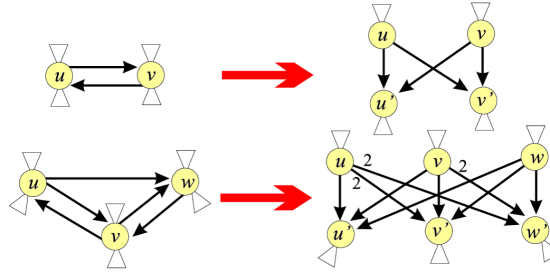
Figure 2: Preprint transformation

The other possibility, since a citation network is usually almost acyclic, is to transform it into an acyclic network

• by identification (shrinking) of cyclic groups (nontrivial strong components), or

• by deleting some arcs, or

• by transformations such as the ’preprint’ transformation (see Figure 2) which is based on the following idea: Each paper from a strong component is duplicated with its ’preprint’ version. The papers inside strong component cite preprints.

Large strong components in citation network are unlikely – their presence usually indicates an error in the data. An exception from this rule is the citation network of High Energy Particle Physics literature [20] from arXiv. In it different versions of the same paper are treated as a unit. This leads to large strongly connected components. The idea of preprint transformation can be used also in this case to eliminate cycles.

6 First Example: SOM citation network

The purpose of this example is not the analysis of the selected citation network on SOM (self-organizing maps) literature [12, 24, 23], but to present typical steps and results in citation network analysis. We made our analysis using program Pajek.

First we test the network for acyclicity. Since in the SOM network there are 11 nontrivial strong components of size 2, see Table 1, we have to transform the network into acyclic one. We decided to do this by shrinking each component into a single vertex. This operation produces some loops that should be removed.

Now, we can compute the citation weights. We selected the SPC (search path count) method. It returns the following results: the network with citation weights on arcs, the main path network and the vector with vertex weights.

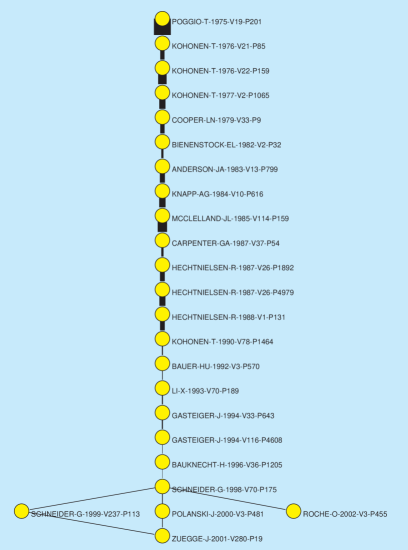
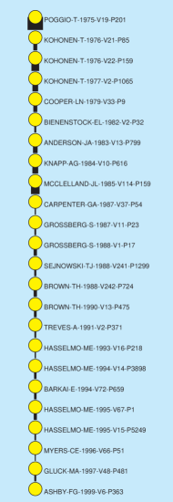
Figure 3: Main path and CPM path in SOM network with SPC weights

In a citation network, a main path (sub)network is constructed starting from the source vertex and selecting at each step in the end vertex/vertices the arc(s) with the highest weight, until a sink vertex is reached.

Another possibility is to apply on the network $\mathbf{N}=(\mathbf{U},R,w)$ the critical path method (CPM) from operations research.

First we draw the main path network. The arc weights are represented by the thickness of arcs. To produce a nice picture of it we apply the Pajek’s macro Layers which contains a sequence of operations for determining a layered layout of an acyclic network (used also in analysis of genealogies represented by p-graphs). Some experiments with settings of different options are needed to obtain a right picture, see left part of Figure 3. In its right part the CPM path is presented.

We see that the upper parts of both paths are identical, but they differ in the continuation. The arcs in the CPM path are thicker.

We could display also the complete SOM network using essentially the same procedure as for the displaying of main path. But the obtained picture would be too complicated (too many vertices and arcs). We have to identify some simpler and important subnetworks inside it.

Inspecting the distribution of values of weights on arcs (lines) we select a threshold 0.007 and determine the corresponding arc-cut – delete all arcs with weights lower than selected threshold and afterwards delete also all isolated vertices (degree $=0$).

Now, we are ready to draw the reduced network. We first produce an automatic layout. We notice some small unimportant components. We preserve only the large main component, draw it and improve the obtained layout manually. To preserve the level structure we use the option that allows only the horizontal movement of vertices.

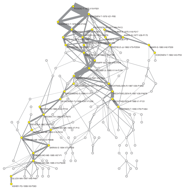
Figure 4: Main subnetwork at level 0.007

Finally we label the ’most important vertices’ with their labels. A vertex is considered important if it is an endpoint of an arc with the weight above the selected threshold (in our case 0.05).

The obtained picture of SOM ’main subnetwork’ is presented in Figure 4. We see that the SOM field evolved in two main branches. From CARPENTER-1987 the strongest (main path) arc is leading to the right branch that after some steps disappears. The left, more vital branch is detected by the CPM path. Further investigation of this is left to the readers with additional knowledge about the SOM field.

Table 2: 15 Hubs and Authorities

Rank	$h$	Hub Id	$a$	Authority Id
1	0.06442	CLARK-JW-1991-V36-P1259	0.85214	HOPFIELD-JJ-1982-V79-P2554
2	0.06366	#GARDNER-E-1988-V21-P257	0.33427	KOHONEN-T-1982-V43-P59
3	0.05794	HUANG-SH-1994-V17-P212	0.14531	KOHONEN-T-1990-V78-P1464
4	0.05721	GULATI-S-1991-V33-P173	0.12398	CARPENTER-GA-1987-V37-P54
5	0.05513	SHUBNIKOV-EI-1997-V64-P989	0.10376	#GARDNER-E-1988-V21-P257
6	0.05496	MARSHALL-JA-1995-V8-P335	0.09353	HOPFIELD-JJ-1986-V233-P625
7	0.05488	VEMURI-V-1993-V36-P203	0.07882	MCELIECE-RJ-1987-V33-P461
8	0.05409	CHENG-B-1994-V9-P2	0.07656	KOHONEN-T-1988-V1-P3
9	0.05360	BUSCEMA-M-1998-V33-P17	0.07372	RUMELHART-DE-1985-V9-P75
10	0.05258	XU-L-1993-V6-P627	0.07271	KOSKO-B-1988-V18-P49
11	0.05249	WELLS-DM-1998-V41-P173	0.07246	ANDERSON-JA-1977-V84-P413
12	0.05233	SCHYNS-PG-1991-V15-P461	0.07033	AMARI-SI-1977-V26-P175
13	0.05173	SMITH-KA-1999-V11-P15	0.06709	KOSKO-B-1987-V26-P4947
14	0.05149	BONABEAU-E-1998-V9-P1107	0.05802	PERSONNAZ-L-1985-V46-PL359
15	0.05126	KOHONEN-T-1990-V78-P1464	0.05702	GROSSBERG-S-1987-V11-P23

As a complementary information we can determine Kleinberg’s hubs and authorities vertex weights [17]. Papers that are cited by many other papers are called authorities; papers that cite many other documents are called hubs. Good authorities are those that are cited by good hubs and good hubs cite good authorities. The 15 highest ranked hubs and authorities are presented in Table 2. We see that the main authorities are located in eighties and the main hubs in nineties. Note that, since we are using the relation $uRv\equiv u\mbox{ is cited by }v$, we have to interchange the roles of hubs and authorities produced by Pajek.

An elaboration of the hubs and authorities approach to the analysis of citation networks complemented with visualization can be found in Brandes and Willhalm (2002) [8].

7 Second Example: US patents

The network of US patents from 1963 to 1999 [21] is an example of very large network (3774768 vertices and 16522438 arcs) that, using some special options in Pajek, can still be analyzed on PC with at least 1 G memory. The SPC weights are determined in a range of 1 minute. This shows that the proposed approach can be used also for very large networks.

The obtained main path and CPM path are presented in Figure 5. Collecting from the United States Patent and Trademark Office [22] the basic data about the patents from both paths, see Table 3-6, we see that they deal with ’liquid crystal displays’.

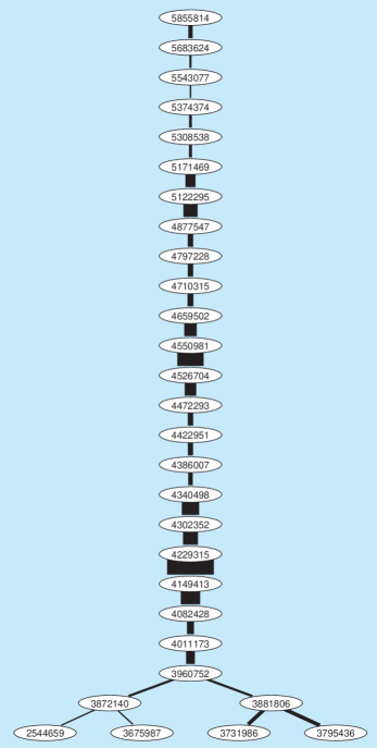
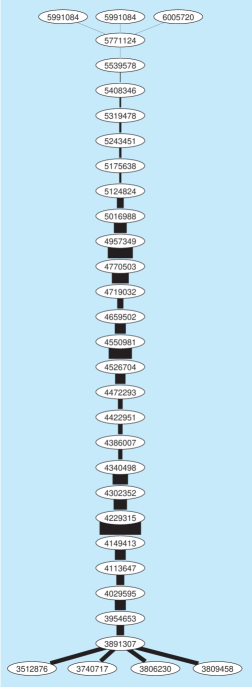
Figure 5: Main path and CPM path subnetwork of Patents

Table 3: Patents on the liquid-crystal display

patent	date	author(s) and title
2544659	Mar 13, 1951	Dreyer. Dichroic light-polarizing sheet and the like and the
		formation and use thereof
2682562	Jun 29, 1954	Wender, et al. Reduction of aromatic carbinols
3322485	May 30, 1967	Williams. Electro-optical elements utilazing an organic
		nematic compound
3512876	May 19, 1970	Marks. Dipolar electro-optic structures
3636168	Jan 18, 1972	Josephson. Preparation of polynuclear aromatic compounds
3666948	May 30, 1972	Mechlowitz, et al. Liquid crystal termal imaging system
		having an undisturbed image on a disturbed background
3675987	Jul 11, 1972	Rafuse. Liquid crystal compositions and devices
3691755	Sep 19, 1972	Girard. Clock with digital display
3697150	Oct 10, 1972	Wysochi. Electro-optic systems in which an electrophoretic-
		like or dipolar material is dispersed throughout a liquid
		crystal to reduce the turn-off time
3731986	May 8, 1973	Fergason. Display devices utilizing liquid crystal light
		modulation
3740717	Jun 19, 1973	Huener, et al. Liquid crystal display
3767289	Oct 23, 1973	Aviram, et al. Class of stable trans-stilbene compounds,
		some displaying nematic mesophases at or near room
		temperature and others in a range up to 100∘C
3773747	Nov 20, 1973	Steinstrasser. Substituted azoxy benzene compounds
3795436	Mar 5, 1974	Boller, et al. Nematogenic material which exhibit the Kerr
		effect at isotropic temperatures
3796479	Mar 12, 1974	Helfrich, et al. Electro-optical light-modulation cell
		utilizing a nematogenic material which exhibits the Kerr
		effect at isotropic temperatures
3806230	Apr 23, 1974	Haas. Liquid crystal imaging system having optical storage
		capabilities
3809458	May 7, 1974	Huener, et al. Liquid crystal display
3872140	Mar 18, 1975	Klanderman, et al. Liquid crystalline compositions and
		method
3876286	Apr 8, 1975	Deutscher, et al. Use of nematic liquid crystalline substances
3881806	May 6, 1975	Suzuki. Electro-optical display device
3891307	Jun 24, 1975	Tsukamoto, et al. Phase control of the voltages applied to
		opposite electrodes for a cholesteric to nematic phase
		transition display
3947375	Mar 30, 1976	Gray, et al. Liquid crystal materials and devices
3954653	May 4, 1976	Yamazaki. Liquid crystal composition having high dielectric
		anisotropy and display device incorporating same
3960752	Jun 1, 1976	Klanderman, et al. Liquid crystal compositions
3975286	Aug 17, 1976	Oh. Low voltage actuated field effect liquid crystals
		compositions and method of synthesis
4000084	Dec 28, 1976	Hsieh, et al. Liquid crystal mixtures for electro-optical
		display devices
4011173	Mar 8, 1977	Steinstrasser. Modified nematic mixtures with
		positive dielectric anisotropy
4013582	Mar 22, 1977	Gavrilovic. Liquid crystal compounds and electro-optic
		devices incorporating them
4017416	Apr 12, 1977	Inukai, et al. P-cyanophenyl 4-alkyl-4’-biphenylcarboxylate,
		method for preparing same and liquid crystal compositions
		using same

Table 4: Patents on the liquid-crystal display

patent	date	author(s) and title
4029595	Jun 14, 1977	Ross, et al. Novel liquid crystal compounds and electro-optic
		devices incorporating them
4032470	Jun 28, 1977	Bloom, et al. Electro-optic device
4077260	Mar 7, 1978	Gray, et al. Optically active cyano-biphenyl compounds and
		liquid crystal materials containing them
4082428	Apr 4, 1978	Hsu. Liquid crystal composition and method
4083797	Apr 11, 1978	Oh. Nematic liquid crystal compositions
4113647	Sep 12, 1978	Coates, et al. Liquid crystalline materials
4118335	Oct 3, 1978	Krause, et al. Liquid crystalline materials of reduced viscosity
4130502	Dec 19, 1978	Eidenschink, et al. Liquid crystalline cyclohexane derivatives
4149413	Apr 17, 1979	Gray, et al. Optically active liquid crystal mixtures and
		liquid crystal devices containing them
4154697	May 15, 1979	Eidenschink, et al. Liquid crystalline hexahydroterphenyl
		derivatives
4195916	Apr 1, 1980	Coates, et al. Liquid crystal compounds
4198130	Apr 15, 1980	Boller, et al. Liquid crystal mixtures
4202791	May 13, 1980	Sato, et al. Nematic liquid crystalline materials
4229315	Oct 21, 1980	Krause, et al. Liquid crystalline cyclohexane derivatives
4261652	Apr 14, 1981	Gray, et al. Liquid crystal compounds and materials and
		devices containing them
4290905	Sep 22, 1981	Kanbe. Ester compound
4293434	Oct 6, 1981	Deutscher, et al. Liquid crystal compounds
4302352	Nov 24, 1981	Eidenschink, et al. Fluorophenylcyclohexanes, the preparation
		thereof and their use as components of liquid crystal dielectrics
4330426	May 18, 1982	Eidenschink, et al. Cyclohexylbiphenyls, their preparation and
		use in dielectrics and electrooptical display elements
4340498	Jul 20, 1982	Sugimori. Halogenated ester derivatives
4349452	Sep 14, 1982	Osman, et al. Cyclohexylcyclohexanoates
4357078	Nov 2, 1982	Carr, et al. Liquid crystal compounds containing an alicyclic
		ring and exhibiting a low dielectric anisotropy and liquid
		crystal materials and devices incorporating such compounds
4361494	Nov 30, 1982	Osman, et al. Anisotropic cyclohexyl cyclohexylmethyl ethers
4368135	Jan 11, 1983	Osman. Anisotropic compounds with negative or positive
		DC-anisotropy and low optical anisotropy
4386007	May 31, 1983	Krause, et al. Liquid crystalline naphthalene derivatives
4387038	Jun 7, 1983	Fukui, et al. 4-(Trans-4’-alkylcyclohexyl) benzoic acid
		4’”-cyano-4”-biphenylyl esters
4387039	Jun 7, 1983	Sugimori, et al. Trans-4-(trans-4’-alkylcyclohexyl)-cyclohexane
		carboxylic acid 4’”-cyanobiphenyl ester
4400293	Aug 23, 1983	Romer, et al. Liquid crystalline cyclohexylphenyl derivatives
4415470	Nov 15, 1983	Eidenschink, et al. Liquid crystalline fluorine-containing
		cyclohexylbiphenyls and dielectrics and electro-optical display
		elements based thereon
4419263	Dec 6, 1983	Praefcke, et al. Liquid crystalline cyclohexylcarbonitrile
		derivatives
4422951	Dec 27, 1983	Sugimori, et al. Liquid crystal benzene derivatives
4455443	Jun 19, 1984	Takatsu, et al. Nematic halogen Compound
4456712	Jun 26, 1984	Christie, et al. Bismaleimide triazine composition
4460770	Jul 17, 1984	Petrzilka, et al. Liquid crystal mixture
4472293	Sep 18, 1984	Sugimori, et al. High temperature liquid crystal substances of
		four rings and liquid crystal compositions containing the same

Table 5: Patents on the liquid-crystal display

patent	date	author(s) and title
4472592	Sep 18, 1984	Takatsu, et al. Nematic liquid crystalline compounds
4480117	Oct 30, 1984	Takatsu, et al. Nematic liquid crystalline compounds
4502974	Mar 5, 1985	Sugimori, et al. High temperature liquid-crystalline ester
		compounds
4510069	Apr 9, 1985	Eidenschink, et al. Cyclohexane derivatives
4514044	Apr 30, 1985	Gunjima, et al. 1-(Trans-4-alkylcyclohexyl)-2-(trans-4’-(p-sub
		stituted phenyl) cyclohexyl)ethane and liquid crystal mixture
4526704	Jul 2, 1985	Petrzilka, et al. Multiring liquid crystal esters
4550981	Nov 5, 1985	Petrzilka, et al. Liquid crystalline esters and mixtures
4558151	Dec 10, 1985	Takatsu, et al. Nematic liquid crystalline compounds
4583826	Apr 22, 1986	Petrzilka, et al. Phenylethanes
4621901	Nov 11, 1986	Petrzilka, et al. Novel liquid crystal mixtures
4630896	Dec 23, 1986	Petrzilka, et al. Benzonitriles
4657695	Apr 14, 1987	Saito, et al. Substituted pyridazines
4659502	Apr 21, 1987	Fearon, et al. Ethane derivatives
4695131	Sep 22, 1987	Balkwill, et al. Disubstituted ethanes and their use in liquid
		crystal materials and devices
4704227	Nov 3, 1987	Krause, et al. Liquid crystal compounds
4709030	Nov 24, 1987	Petrzilka, et al. Novel liquid crystal mixtures
4710315	Dec 1, 1987	Schad, et al. Anisotropic compounds and liquid crystal
		mixtures therewith
4713197	Dec 15, 1987	Eidenschink, et al. Nitrogen-containing heterocyclic compounds
4719032	Jan 12, 1988	Wachtler, et al. Cyclohexane derivatives
4721367	Jan 26, 1988	Yoshinaga, et al. Liquid crystal device
4752414	Jun 21, 1988	Eidenschink, et al. Nitrogen-containing heterocyclic compounds
4770503	Sep 13, 1988	Buchecker, et al. Liquid crystalline compounds
4795579	Jan 3, 1989	Vauchier, et al. 2,2’-difluoro-4-alkoxy-4’-hydroxydiphenyls and
		their derivatives, their production process and
		their use in liquid crystal display devices
4797228	Jan 10, 1989	Goto, et al. Cyclohexane derivative and liquid crystal
		composition containing same
4820839	Apr 11, 1989	Krause, et al. Nitrogen-containing heterocyclic esters
4832462	May 23, 1989	Clark, et al. Liquid crystal devices
4877547	Oct 31, 1989	Weber, et al. Liquid crystal display element
4957349	Sep 18, 1990	Clerc, et al. Active matrix screen for the color display of
		television pictures, control system and process for producing
		said screen
5016988	May 21, 1991	Iimura. Liquid crystal display device with a birefringent
		compensator
5016989	May 21, 1991	Okada. Liquid crystal element with improved contrast and
		brightness
5122295	Jun 16, 1992	Weber, et al. Matrix liquid crystal display
5124824	Jun 23, 1992	Kozaki, et al. Liquid crystal display device comprising a
		retardation compensation layer having a maximum principal
		refractive index in the thickness direction
5171469	Dec 15, 1992	Hittich, et al. Liquid-crystal matrix display
5175638	Dec 29, 1992	Kanemoto, et al. ECB type liquid crystal display device having
		birefringent layer with equal refractive indexes in the thickness
		and plane directions

Table 6: Patents on the liquid-crystal display

patent	date	author(s) and title
5243451	Sep 7, 1993	Kanemoto, et al. DAP type liquid crystal device with cholesteric
		liquid crystal birefringent layer
5283677	Feb 1, 1994	Sagawa, et al. Liquid crystal display with ground regions
		between terminal groups
5308538	May 3, 1994	Weber, et al. Supertwist liquid-crystal display
5319478	June 7, 1994	Funfschilling, et al. Light control systems with a circular polarizer
		and a twisted nematic liquid crystal having a minimum path
		difference of .lambda./2
5374374	Dec 20, 1994	Weber, et al. Supertwist liquid-crystal display
5408346	Apr 18, 1995	Trissel, et al. Optical collimating device employing cholesteric
		liquid crystal and a non-transmissive reflector
5539578	Jul 23, 1996	Togino, et al. Image display apparatus
5543077	Aug 6, 1996	Rieger, et al. Nematic liquid-crystal composition
5555116	Sep 10, 1996	Ishikawa, et al. Liquid crystal display having adjacent
		electrode terminals set equal in length
5683624	Nov 4, 1997	Sekiguchi, et al. Liquid crystal composition
5771124	Jun 23, 1998	Kintz, et al. Compact display system with two stage magnification
		and immersed beam splitter
5855814	Jan 5, 1999	Matsui, et al. Liquid crystal compositions and liquid crystal
		display elements
5991084	Nov 23, 1999	Hildebrand, et al. Compact compound magnified virtual image
		display with a reflective/transmissive optic
6005720	Dec 21, 1999	Watters, et al. Reflective micro-display system

But, in this network there should be thousands of ’themes’. How to identify them? Using the arc weights we can define a theme as a connected small subnetwork of size in the interval $k$ .. $K$ (for example, between $k=\frac{1}{3}h$ and $K=3h$) with stronger internal cohesion relatively to its neighborhood.

To find such subnetworks we use again the arc-cuts. We select a treshold $t$ and delete all arcs with weight lower than $t$. In the so reduced network we determine (weakly) connected components. The components of size in range $k..K$, we call them $(k,K)$-islands, represent the themes since:

• they are connected and of selected size,

• all arcs linking them to their outside neighbors have weight lower than $t$, and

• each vertex of an island is linked with some other vertex in the same island with an arc with a weight at least $t$.

We discard components of size smaller than $k$ as ’noninteresting’.

The components of size larger then $K$ are too large. They contain several themes. To identify them we repeat the procedure on the network of these components with a higher threshold value $t^{\prime}$. Recently we developed an algorithm, named Islands [7], that by ’continuosly’ changing the threshold identifies all maximal $(k,K)$-islands.

We determined for SPC weights all (2,90)-islands in the US Patents network. The reduced network of islands has 470137 vertices, 307472 arcs and for different $k$: $C_{2}=$187610, $C_{5}=$8859,$C_{30}=$101, $C_{50}=$30 islands. The detailed island size frequency distribution is given in Table 7 and presented in a log-log scale in Figure 6 that shows that it obeys the power law.

Table 7: Island size frequency distribution

         [1]   0 139793  29670 9288 3966 1827 997 578 362 250
        [11] 190    125    104   71   47   37  36  33  21  23
        [21]  17     16      8    7   13   10  10   5   5   5
        [31]  12      3      7    3    3    3   2   6   6   2
        [41]   1      3      4    1    5    2   1   1   1   1
        [51]   2      3      3    2    0    0   0   0   0   1
        [61]   0      0      0    0    1    0   0   2   0   0
        [71]   0      0      1    1    0    0   0   1   0   0
        [81]   2      0      0    0    0    1   2   0   0   7

Figure 6: Island size frequency distribution

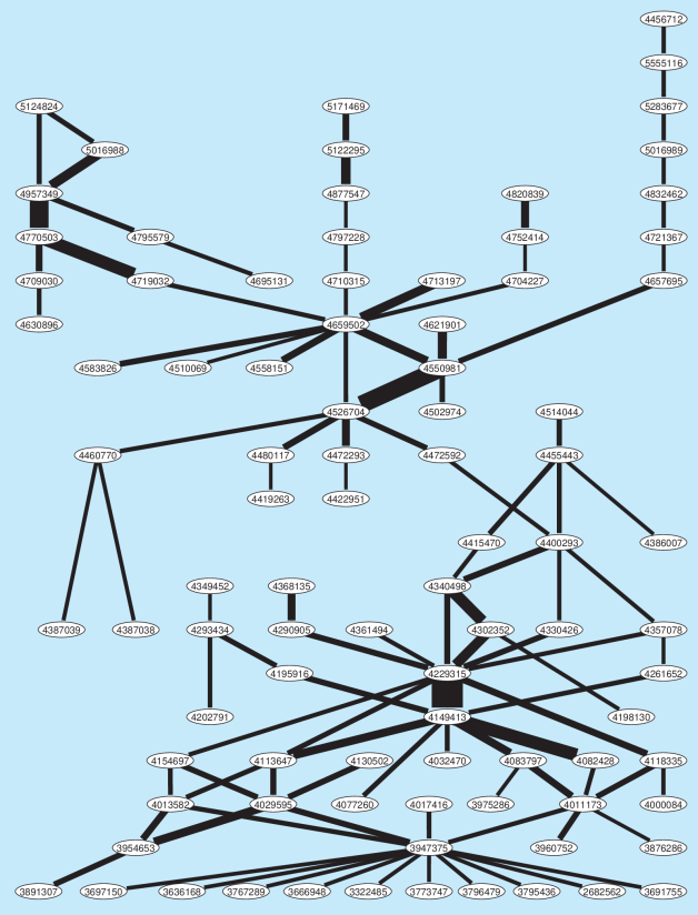
Figure 7: Main island ’liquid-crystal display’

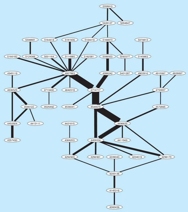
Figure 8: Island ’producing a foam’

Table 8: Some patents from the ’foam’ island

patent	date	author(s) and title
4060439	Nov 29, 1977	Rosemund, et al. Polyurethane foam composition and method of
		making same
4292369	Sep 29, 1981	Ohashi, et al. Fireproof laminates
4357430	Nov 2, 1982	VanCleve. Polymer/polyols, methods for making same and
		polyurethanes based thereon
4459334	Jul 10, 1984	Blanpied, et al. Composite building panel
4496625	Jan 29, 1985	Snider , et al. Alkoxylated aromatic amine-aromatic polyester
		polyol blend and polyisocyanurate foam therefrom
4544679	Oct 1, 1985	Tideswell, et al. Polyol blend and polyisocyanurate foam
		produced therefrom
4714717	Dec 22, 1987	Londrigan, et al. Polyester polyols modified by low molecular
		weight glycols and cellular foams therefrom
4927863	May 22, 1990	Bartlett, et al. Process for producing closed-cell polyurethane
		foam compositions expanded with mixtures of blowing agents
4996242	Feb 26, 1991	Lin. Polyurethane foams manufactured with mixed
		gas/liquid blowing agents
5169873	Dec 8, 1992	Behme, et al. Process for the manufacture of foams with the aid
		of blowing agents containing fluoroalkanes and fluorinated
		ethers, and foams obtained by this process
5187206	Feb 16, 1993	Volkert, et al. Production of cellular plastics by the
		polyisocyanate polyaddition process, and low-boiling,
		fluorinated or perfluorinated, tertiary alkylamines
		as blowing agent-containing emulsions for this purpose
5308881	May 3, 1994	Londrigan, et al. Surfactant for polyisocyanurate foams
		made with alternative blowing agents
5558810	Sep 24, 1996	Minor, et al. Pentafluoropropane compositions

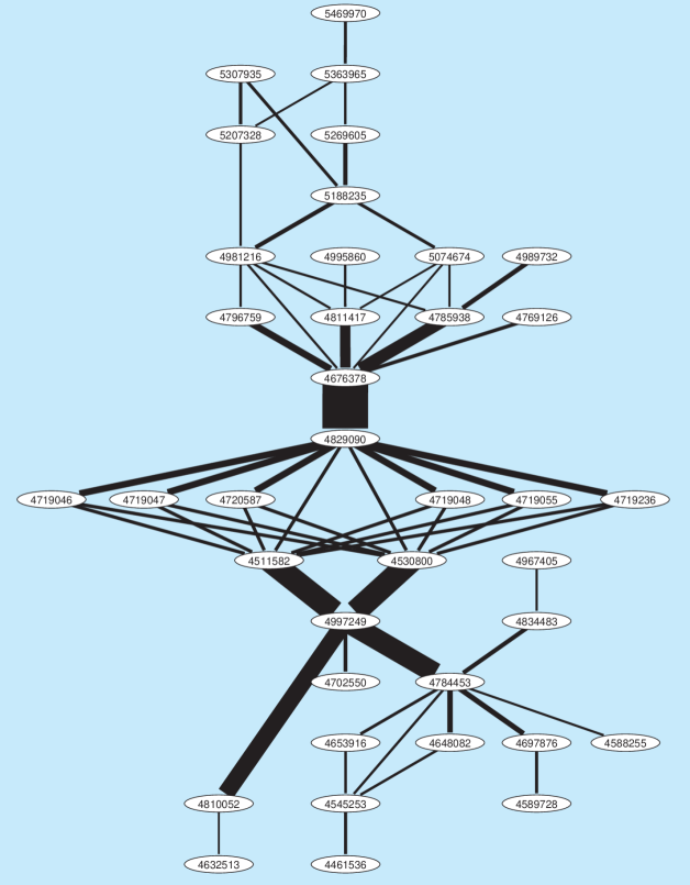
Figure 9: Island ’fiber optics and bags’

Table 9: Some patents from ’fiber optics and bags’ island

patent	date	author(s) and title
4461536	Jul 24, 1984	Shaw, et al. Fiber coupler displacement transducer
4511582	Apr 16, 1985	Bair. Phenanthrene derivatives
4530800	Jul 23, 1985	Bair. Perylene derivatives
4589728	May 20, 1986	Dyott, et al. Optical fiber polarizer
4676378	Jun 30, 1987	Baxley, et al. Bag pack
4719047	Jan 12, 1988	Bair. Anthracene derivatives
4784453	Nov 15, 1988	Shaw, et al. Backward-flow ladder architecture and method
4785938	Nov 22, 1988	Benoit, Jr., et al. Thermoplastic bag pack
4810052	Mar 7, 1989	Fling. Fiber optic bidirectional data bus tap
4811417	Mar 7, 1989	Prince, et al. Handled bag with supporting slits in handle
4829090	May 9, 1989	Bair. Chrysene derivatives
4981216	Jan 1, 1991	Wilfong, Jr. Easy opening bag pack and supporting rack
		system and fabricating method
4997249	Mar 5, 1991	Berry, et al. Variable weight fiber optic transversal filter
5188235	Feb 23, 1993	Pierce, et al. Bag pack
5307935	May 3, 1994	Kemanjian. Packs of self opening plastic bags and method of
		fabricating the same
5363965	Nov 15, 1994	Nguyen. Self-opening thermoplastic bag system

The main island has 90 vertices and contains middle parts of the main path and the CPM path. They also have a short common part. Again, the greedy strategy of the main path leads to a less vital branch. Considering the basic data about the patents from Table 3-5, we see that also the main island deals with ’liquid crystal displays’.

For additional illustration of results obtained by Islands algorithm we selected two smaller islands at lower levels – see Figure 8 (50 vertices) and Figure 9 (38 vertices). Retreiving the basic data about some patents in these islands from United States Patent and Trademark Office, see Table 8 and Table 9, we can label the corresponding theme of the first island as ’producing a foam’. The theme of the second island deals initially with ’fiber optics’, but in the upper part it switches to ’bag pack system’.

8 Conclusions

In the paper we proposed an approach to the analysis of citation networks that can be used also for very large networks with millions of vertices and arcs.

On test cases, the methods SPC, SPLC, NPPC produced almost the same results. Since the method SPC has additional ’nice’ properties it could be considered as a ’first choice’ – but, to make a grounded recommendation, additional experiences should be gained from the analyses of real-life large citation networks.

The granularity of the results strongly depends on the range for ’interesting themes’ $k$ .. $K$ – varying these two parameters we get larger or smaller sets of themes.

Instead of arc-cuts we could consider also vertex-cuts with respect to $p$-cores on SPC weights [6] with a $p$-function

$$p(v,W)=\max(\sum_{u\in W:uRv}w(u,v),\sum_{u\in W:vRu}w(v,u))$$

The subnetworks approach only filters out the structurally important subnetworks thus providing a researcher with a smaller manageable structures which can be further analyzed using more sophisticated and/or substantial methods.

9 Acknowledgments

The search path count algorithm was developed during my visit in Pittsburgh in 1991 and presented at the Network seminar [2]. It was presented to the broader audience at EASST’94 in Budapest [3]. In 1997 it was included in program Pajek [4]. The ’preprint’ transformation was developed as a part of the contribution for the Graph drawing contest 2001 [5]. The algorithm for the path length counts was developed in August 2002 and the Islands algorithm in August 2003.

The author would like to thank Patrick Doreian and Norm Hummon for introducing him into the field of citation network analysis, Eugene Garfield for making available the data on real-life networks and providing some relevant references, and Andrej Mrvar and Matjaž Zaveršnik for implementing the algorithms in Pajek.

This work was supported by the Ministry of Education, Science and Sport of Slovenia, Project 0512-0101.

References

- [1] Asimov I.: The Genetic Code, New American Library, New York, 1963.
- [2] Batagelj V.: Some Mathematics of Network Analysis. Network Seminar, Department of Sociology, University of Pittsburgh, January 21, 1991.
- [3] Batagelj V.: An Efficient Algorithm for Citation Networks Analysis. Paper presented at EASST’94, Budapest, Hungary, August 28-31, 1994.
-
[4]
Batagelj V., Mrvar A.: Pajek – program for
analysis and visualization of large networks.
http://vlado.fmf.uni-lj.si/pub/networks/pajek/
http://vlado.fmf.uni-lj.si/pub/networks/pajek/howto/extreme.htm -
[5]
Batagelj V., Mrvar A.:
Graph Drawing Contest 2001 Layouts
http://vlado.fmf.uni-lj.si/pub/GD/GD01.htm -
[6]
Batagelj V., Zaveršnik M.:
Generalized Cores. Submitted, 2002.
http://arxiv.org/abs/cs.DS/0202039 - [7] Batagelj V., Zaveršnik M.: Islands – identifying themes in large networks. In preparation, August 2003.
-
[8]
Brandes U., Willhalm T.:
Visualization of
bibliographic networks with a reshaped landscape metaphor.
Joint Eurographics – IEEE TCVG Symposium on Visualization,
D. Ebert, P. Brunet, I. Navazo (Editors), 2002.
http://algo.fmi.uni-passau.de/~brandes/
publications/bw-vbnrl-02.pdf - [9] Cormen T.H., Leiserson C.E., Rivest R.L., Stein C.: Introduction to Algorithms, Second Edition. MIT Press, 2001.
-
[10]
Garfield E, Sher IH, and Torpie RJ.:
The Use of Citation Data in Writing the History of Science.
Philadelphia: The Institute for Scientific Information, December 1964.
http://www.garfield.library.upenn.edu/papers/
useofcitdatawritinghistofsci.pdf -
[11]
Garfield E.:
From Computational Linguistics to Algorithmic Historiography,
paper presented at the Symposium in Honor of Casimir Borkowski
at the University of Pittsburgh School of Information Sciences,
September 19, 2001.
http://garfield.library.upenn.edu/papers/pittsburgh92001.pdf -
[12]
Garfield E., Pudovkin A.I., Istomin, V.S.:
Histcomp – (compiled Historiography program)
http://garfield.library.upenn.edu/histcomp/guide.html
http://www.garfield.library.upenn.edu/histcomp/index.html -
[13]
Garner R.:
A computer oriented, graph theoretic analysis of citation index structures.
Flood B. (Editor), Three Drexel information science studies, Philadelphia:
Drexel University Press 1967.
http://www.garfield.library.upenn.edu/rgarner.pdf - [14] Hummon N.P., Doreian P.: Connectivity in a Citation Network: The Development of DNA Theory. Social Networks, 11(1989) 39-63.
- [15] Hummon N.P., Doreian P.: Computational Methods for Social Network Analysis. Social Networks, 12(1990) 273-288.
- [16] Hummon N.P., Doreian P., Freeman L.C.: Analyzing the Structure of the Centrality-Productivity Literature Created Between 1948 and 1979. Knowledge: Creation, Diffusion, Utilization, 11(1990)4, 459-480.
-
[17]
Kleinberg J.:
Authoritative sources in a hyperlinked environment.
In Proc 9th ACMSIAM Symposium on Discrete Algorithms, 1998, p. 668-677.
http://www.cs.cornell.edu/home/kleinber/auth.ps
http://citeseer.nj.nec.com/kleinberg97authoritative.html - [18] Wilson, R.J., Watkins, J.J.: Graphs: An Introductory Approach. New York: John Wiley and Sons, 1990.
-
[19]
Pajek’s datasets – citation networks:
http://vlado.fmf.uni-lj.si/pub/networks/data/cite/ -
[20]
KDD Cup 2003:
http://www.cs.cornell.edu/projects/kddcup/index.html
http://arxiv.org/ -
[21]
Hall, B.H., Jaffe, A.B. and Tratjenberg M.:
The NBER U.S. Patent Citations Data File. NBER Working Paper 8498 (2001).
http://www.nber.org/patents/ -
[22]
The United States Patent and Trademark Office.
http://patft.uspto.gov/netahtml/srchnum.htm -
[23]
Bibliography on the Self-Organizing Map (SOM) and Learning Vector Quantization (LVQ)
http://liinwww.ira.uka.de/bibliography/Neural/SOM.LVQ.html -
[24]
Neural Networks Research Centre: Bibliography of SOM papers.
http://www.cis.hut.fi/research/refs/