On Applying Or-Parallelism and Tabling to Logic Programs

Abstract

Logic Programming languages, such as Prolog, provide a high-level, declarative approach to programming. Logic Programming offers great potential for implicit parallelism, thus allowing parallel systems to often reduce a program’s execution time without programmer intervention. We believe that for complex applications that take several hours, if not days, to return an answer, even limited speedups from parallel execution can directly translate to very significant productivity gains.

It has been argued that Prolog’s evaluation strategy – SLD resolution – often limits the potential of the logic programming paradigm. The past years have therefore seen widening efforts at increasing Prolog’s declarativeness and expressiveness. Tabling has proved to be a viable technique to efficiently overcome SLD’s susceptibility to infinite loops and redundant subcomputations.

Our research demonstrates that implicit or-parallelism is a natural fit for logic programs with tabling. To substantiate this belief, we have designed and implemented an or-parallel tabling engine – OPTYap – and we used a shared-memory parallel machine to evaluate its performance. To the best of our knowledge, OPTYap is the first implementation of a parallel tabling engine for logic programming systems. OPTYap builds on Yap’s efficient sequential Prolog engine. Its execution model is based on the SLG-WAM for tabling, and on the environment copying for or-parallelism.

Preliminary results indicate that the mechanisms proposed to parallelize search in the context of SLD resolution can indeed be effectively and naturally generalized to parallelize tabled computations, and that the resulting systems can achieve good performance on shared-memory parallel machines. More importantly, it emphasizes our belief that through applying or-parallelism and tabling to logic programs the range of applications for Logic Programming can be increased.

1 Introduction

Logic programming provides a high-level, declarative approach to programming. Arguably, Prolog is the most popular and powerful logic programming language. Prolog’s popularity was sparked by the success of the sequential execution model presented in 1983 by David H. D. Warren, the Warren Abstract Machine (WAM) [56]. Throughout its history, Prolog has demonstrated the potential of logic programming in application areas such as Artificial Intelligence, Natural Language Processing, Knowledge Based Systems, Machine Learning, Database Management, or Expert Systems.

Logic programs are written in a subset of First-Order Logic, Horn clauses, that has an intuitive interpretation as positive facts and as rules. Programs use the logic to express the problem, whilst questions are answered by a resolution procedure with the aid of user annotations. The combination was summarized by Kowalski’s motto [23]:

$$algorithm~{}=~{}logic~{}+control$$

Ideally, one would want Prolog programs to be written as logical statements first, and for control to be tackled as a separate issue. In practice, the limitations of Prolog’s operational semantics, SLD resolution, mean that Prolog programmers must be concerned with SLD semantics throughout program development.

Several proposals have been put forth to overcome some of these limitations and therefore improve the declarativeness and expressiveness of Prolog. One such proposal that has been gaining in popularity is tabling, also referred to as tabulation or memoing [29]. In a nutshell, tabling consists of storing intermediate answers for subgoals so that they can be reused when a repeated subgoal appears during the resolution process. It can be shown that tabling based execution models, such as SLG resolution [8], are able to reduce the search space, avoid looping, and that they have better termination properties than SLD based models. For instance, SLG resolution is guaranteed to terminate for all logical programs with the bounded term-size property [8].

Work on SLG resolution, as implemented in the XSB logic programming system [53], proved the viability of tabling technology for applications such as Natural Language Processing, Knowledge Based Systems and Data Cleaning, Model Checking, and Program Analysis. SLG resolution also includes several extensions to Prolog, namely support for negation [4], hence allowing for novel applications in the areas of Non-Monotonic Reasoning and Deductive Databases.

One of the major advantages of logic programming is that it is well suited for parallel execution. The interest in the parallel execution of logic programs mainly arose from the fact that parallelism can be exploited implicitly from logic programs. This means that parallelism can be automatically exploited, that is, without input from the programmer to express or manage parallelism, ideally making parallel logic programming as easy as logic programming.

Logic programming offers two major forms of implicit parallelism, Or-Parallelism and And-Parallelism. Or-parallelism results from the parallel execution of alternative clauses for a given predicate goal, while and-parallelism stems from the parallel evaluation of subgoals in an alternative clause. Some of the most well-known systems that successfully supported these forms of parallelism are: Aurora [26] and Muse [2] for or-parallelism; &-Prolog [20], DASWAM [47], and ACE [31] for and-parallelism; and Andorra-I [46] for or-parallelism together with and-parallelism. A detailed presentation of such systems and the challenges and problems in their implementation can be found in [17]. Arguably, or-parallel systems have been the most successful parallel logic programming systems so far. Experience has shown that or-parallel systems can obtain very good speedups for applications that require search. Examples can be found in application areas such Parsing, Optimization, Structured Database Querying, Expert Systems and Knowledge Discovery applications.

The good results obtained with parallelism and with tabling rises the question of whether further efficiency improvements may be achievable through parallelism. Freire and colleagues were the first to research this area [13]. Although tabling works for both deterministic and non-deterministic applications, Freire focused on the search process, because tabling has frequently been used to reduce the search space. In their model, each tabled subgoal is computed independently in a separate computational thread, a generator thread. Each generator thread is the sole responsible for fully exploiting its subgoal and obtain the complete set of answers. Arguably, Freire’s model will work particularly well if we have many non-deterministic generators. On the other hand, it will not exploit parallelism if there is a single generator and many non-tabled subgoals. It also does not exploit parallelism between a generator’s clauses. As we discuss in Section 7, experience has shown that interesting applications do indeed have a limited number of generators.

Ideally, we would like to exploit maximum parallelism and take maximum advantage of current technology for tabling and parallel systems. To exploit maximum parallelism, we would like to exploit parallelism from both tabled and non-tabled subgoals. Further, we would like to reuse existing technology for tabling and parallelism. As such, we would like to exploit parallelism from tabled and non-tabled subgoals in much the same way. As with Freire, we would focus on or-parallelism first, and we will focus throughout on shared-memory platforms.

Towards this goal, we proposed two new computational models [37], Or-Parallelism within Tabling (OPT) and Tabling within Or-Parallelism (TOP). Both models are based on the idea that all open alternatives in the search tree should be amenable to parallel exploitation, be they from tabled or non-tabled subgoals. The OPT model further assumes tabling as the base component of the parallel system, that is, each worker is a full sequential tabling engine. OPT triggers or-parallelism when workers run out of alternatives to exploit: at this point, a worker will share part of its SLG derivations with the other. In contrast, the TOP model represents the whole SLG forest as a shared search tree, thus unifying parallelism with tabling. Workers are logically positioned at branches in this tree. When a branch completes or suspends, workers move to nodes with open alternatives, that is, alternatives with either open clauses or new answers stored in the table.

The main contribution of this work is the design and performance evaluation of what to the best of our knowledge is the first parallel tabling logic programming system, OPTYap [40]. We chose the OPT model for two main advantages, both stemming from the fact that OPT encapsulates or-parallelism within tabling. First, implementation of the OPT models follows naturally from two well-understood implementation issues: we need to implement a tabling engine, and then we need to support or-parallelism. Second, in the OPT model a worker can keep its nodes private until reaching a sharing point. This is a key issue in reducing parallel overheads. We remark that it is common in or-parallel works to say that work is initially private, and that is made public after sharing.

OPTYap builds on the YapOr [38] and YapTab [39] engines. YapOr was previous work on supporting or-parallelism over Yap’s Prolog system [45]. YapOr is based on the environment copying model for shared-memory machines, as originally implemented in Muse [1]. YapTab is a sequential tabling engine that extends Yap’s execution model to support tabled evaluation for definite programs. YapTab’s implementation is largely based on the ground-breaking design of the XSB system [43, 35], which implements the SLG-WAM [49, 44, 42]. YapTab has been designed from scratch and its development was done taking into account the major purpose of further integration to achieve an efficient parallel tabling computational model, whilst comparing favorably with current state of the art technology. In other words, we aim at respecting the no-slowdown principle [19]: our or-parallel tabling system should, when executed with a single worker, run as fast or faster than the current available sequential tabling systems. Otherwise, parallel performance results would not be significant and fair.

In order to validate our design we studied in detail the performance of OPTYap in shared-memory machines up to 32 workers. The results we gathered show that OPTYap does indeed introduce low overheads for sequential execution and that it compares favorably with current versions of XSB. Furthermore, the results show that OPTYap maintains YapOr’s speedups for parallel execution of non-tabled programs, and that there are tabled applications that can achieve very high performance through parallelism. This substantiates our belief that tabling and parallelism can together contribute to increasing the range of applications for Logic Programming.

2 Tabling for Logic Programs

The basic idea behind tabling is straightforward: programs are evaluated by storing newly found answers of current subgoals in an appropriate data space, called the table space. The method then uses this table to verify whether calls to subgoals are repeated. Whenever such a repeated call is found, the subgoal’s answers are recalled from the table instead of being re-evaluated against the program clauses. In practice, two major issues have to be addressed:

1. What is a repeated subgoal? We may say that a subgoal repeats if it is the same as a previous subgoal, up to variable renaming; alternatively, we may say it is repeated if it is an instance of a previous subgoal. The former approach is known as variant-based tabling [33], the latter as subsumption-based tabling [34]. Variant-based tabling has been researched first and is arguably better understood, although there has been significant recent progress in subsumption-based tabling [22]. We shall use variant-based tabling approach in this work.

2. How to execute subgoals? Clearly, we must change the selection function and search rule to accommodate for repeated subgoals. In particular, we must address the situation where we recursively call a tabled subgoal before we have fully tabled all its answers. Several strategies to do so have been proposed [50, 55, 8]. We use the popular SLG resolution [8] in this work, mainly because this approach has good termination properties.

In the following, we illustrate the main principles of tabled evaluation using SLG resolution through an example.

2.1 Tabled Evaluation

Consider the Prolog program of Figure 1. The program defines a small directed graph, represented by the arc/2 predicate, with a relation of reachability, given by the path/2 predicate. In this example we ask the query goal ?- path(a,Z) on this program. Note that traditional Prolog would immediately enter an infinite loop because the first clause of path/2 leads to a repeated call to path(a,Z). In contrast, if tabling is applied then termination is ensured. The declaration :- table path/2 in the program code indicates that predicate path/2 should be tabled. Figure 1 illustrates the evaluation sequence when using tabling.

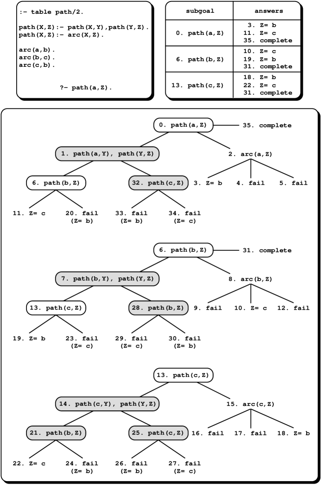
Figure 1: A finite tabled evaluation.

At the top, the figure illustrates the program code and the state of the table space at the end of the evaluation. The main sub-figure shows the forest of SLG trees for the original query. The topmost tree represents the original invocation of the tabled subgoal path(a,Z). It thus computes all nodes reachable from node a. As we shall see, computing all nodes reachable from a requires computing all nodes reachable from b and all nodes reachable from c. The middle tree represents the SLG tree path(b,Z), that is, it computes all nodes reachable from node b. The bottommost tree represents the SLG tree path(c,Z).

Next, we describe in detail the evaluation sequence presented in the figure. For simplicity of presentation, the root nodes of the SLG trees path(b,Z) and path(c,Z), nodes $6$ and $13$, are shown twice. The numbering of nodes denotes the evaluation sequence.

Whenever a tabled subgoal is first called, a new tree is added to the forest of trees and a new entry is added to the table space. We name first calls to tabled subgoals generator nodes (nodes depicted by white oval boxes). In this case, execution starts with a generator node, node $0$. The evaluation thus begins by creating a new tree rooted by path(a,Z) and by inserting a new entry in the table space for it.

The second step is to resolve path(a,Z) against the first clause for path/2, creating node $1$. Node $1$ is a variant call to path(a,Z). We do not resolve the subgoal against the program at these nodes, instead we consume answers from the table space. Such nodes are thus called consumer nodes (nodes depicted by gray oval boxes). At this point, the table does not have answers for this call. The consumer therefore must suspend, either by freezing the whole stacks [42], or by copying the stacks to separate storage [12].

The only possible move after suspending is to backtrack to node $0$. We then try the second clause to path/2, thus calling arc(a,Z). The arc/2 predicate is not tabled, hence it must be resolved against the program, as Prolog would. We name such nodes interior nodes. The first clause for arc/2 immediately succeeds (step $3$). We return back to the context for the original goal, obtaining an answer for path(a,Z), and store the answer Z=b in the table.

We can now choose between two options. We may backtrack and try the alternative clauses for arc/2. Otherwise, we may suspend the current execution, and resume node $1$ with the newly found answer. We decide to continue exploiting the interior node. Both steps $4$ and $5$ fail, so we backtrack to node $0$. Node $0$ has no more clauses left to try, so we try to check whether it has completed. It has not, as node $1$ has not consumed all its answers. We therefore must resume node $1$. The stacks are thus restored to their state at node $1$, and the answer Z=b is forwarded to this node. The subgoal succeeds trivially and we call the continuation, path(b,Z). This is the first call to path(b,Z), so we must create a new tree rooted by path(b,Z) (node $6$), insert a new entry in the table space for it, and proceed with the evaluation of path(b,Z), as shown in the middle tree.

Again, path(b,Z) calls itself recursively, and suspends at node $7$. We now have two consumers, node $1$ and node $7$. The only answer in the table was already consumed, so we have to backtrack to node $6$. This leads to generating a new interior node (node $8$) and consulting the program for clauses to arc(b,Z). The first clause fails (step $9$), but the second clause matches (step $10$). The answer is returned to node $6$ and stored in the table. We next have three choices: continue forward execution, backtrack to the open interior node, or resume the consumer node $7$. In the example we choose to follow a Prolog-like strategy and continue forward execution. Step $11$ thus returns the binding Z=c to the subgoal path(a,Z). We store this answer in path(a,Z)’s table entry.

This will be the last answer to path(a,Z), but we can only prove so after fully exploiting the tree: we still have an open interior node (node $8$), and two suspended consumers (nodes $1$ and $7$). We now choose to backtrack to node $8$, and exploit the last clause for arc/2 (step $12$). At this point we fail all the way back to node $6$. We cannot complete node $6$ yet, as we have an unfinished consumer below (node $7$). The only answer in the table for this consumer is Z=c. We use this answer and obtain a first call to path(c,Z).

The new generator, node $13$, needs a new table. Again, we try the first clause and suspend on the recursive call (node $14$). Next, we backtrack to the second clause. Resolution on arc(c,Z) (node $15$) fails twice (steps $16$ and $17$), and then generates an answer, Z=b (step $18$). We return the answer to node $13$, and store the answer in the table. Again, we choose to continue forward execution, thus finding a new answer to path(b,Z), which is again stored in the table (step $19$). Next, we continue forward execution (step $20$), and find an answer to path(a,Z), Z=b. This answer had already been found at step $3$. SLG resolution does not store duplicate answers in the table. Instead, repeated answers fail. This is how the SLG-WAM avoids unnecessary computations, and even looping in some cases.

What to do next? We do not have interior nodes to exploit, so we backtrack to generator node $13$. The generator cannot complete because it has a consumer below (node $14$). We thus try to complete by sending answers to consumer node $14$. The first answer, Z=b, leads to a new consumer for path(b,Z) (node $21$). The table has two answers for path(b,Z), so we can continue the consumer immediately. This gives a new answer Z=c to path(c,Z), which is stored in the table (step $22$). Continuing forward execution results in the answer Z=c to path(b,Z) (step $23$). This answer repeats what we found in step $10$, so we must fail at this point. Backtracking sends us back to consumer node $21$. We then consume the second answer for path(b,Z), which generates a repeated answer, so we fail again (step $24$). We then try consumer node $14$. It next consumes the second answer, again leading to repeated subgoals, as shown in steps $25$ to $27$. At this point we fail back to node $13$, which makes sure that all answers to the consumers below (nodes $14$, $21$, and $25$) have been tried. Unfortunately, node $13$ cannot complete, because it depends on subgoal path(b,Z) (node $21$). Completing path(c,Z) earlier is not safe because we can loose answers. Note that, at this point, new answers can still be found for subgoal path(b,Z). If new answers are found, consumer node $21$ should be resumed with the newly found answers, which in turn can lead to new answers for subgoal path(c,Z). If we complete sooner, we can loose such answers.

Execution thus backtracks and we try the answer left for consumer node $7$. Steps $28$ to $30$ show that again we only get repeated answers. We fail and return to node $6$. All nodes in the trees for node $6$ and node $13$ have been exploited. As these trees do not depend on any other tree, we are sure no more answers are forthcoming, so at last step $31$ declares the two trees to be complete, and closes the corresponding table entries.

Next we backtrack to consumer node $1$. We had not tried Z=c on this node, but exploiting this answer leads to no further answers (steps $32$ to $34$). The computation has thus fully exploited every node, and we can complete the remaining table entry (step $35$).

2.2 SLG-WAM Operations

The example showed four new main operations: entering a tabled subgoal; adding a new answer to a generator; exporting an answer from the table; and trying to complete the tree. In more detail:

1. The tabled subgoal call operation is a call to a tabled subgoal. It checks if a subgoal is in the table, and if not, adds a new entry for it and allocates a new generator node (nodes $0$, $6$ and $13$). Otherwise, it allocates a consumer node and starts consuming the available answers (nodes $1$, $7$, $14$, $21$, $25$, $28$ and $32$).

2. The new answer operation returns a new answer to a generator. It verifies whether a newly generated answer is already in the table, and if not, inserts it (steps $3$, $10$, $11$, $18$, $19$ and $22$). Otherwise, it fails (steps $20$, $23$, $24$, $26$, $27$, $29$, $30$, $33$, and $34$).

3. The answer resolution operation forwards answers from the table to a consumer node. It verifies whether newly found answers are available for a particular consumer node and, if any, consumes the next one. Otherwise, it schedules a possible resolution to continue the execution. Answers are consumed in the same order they are inserted in the table. The answer resolution operation is executed every time the computation reaches a consumer node.

4. The completion operation determines whether a tabled subgoal is completely evaluated. It executes when we backtrack to a generator node and all of its clauses have been tried. If the subgoal has been completely evaluated, the operation closes its table entry and reclaims space (steps $31$ and $35$). Otherwise, it schedules a possible resolution to continue the execution.

The example also shows that we have some latitude on where and when to apply these operations. The actual sequence of operations thus depends on a scheduling strategy. We next discuss the main principles for completion and scheduling strategies in some more detail.

2.3 Completion

Completion is needed in order to recover space and to support negation. We are most interested on space recovery in this work. Arguably, in this case we could delay completion until the very end of execution. Unfortunately, doing so would also mean that we could only recover space for suspended (consumer) subgoals at the very end of the execution. Instead we shall try to achieve incremental completion [7] to detect whether a generator node has been fully exploited, and if so to recover space for all its consumers.

Completion is hard because a number of generators may be mutually dependent. Figure 2 shows the dependencies for the completed graph. Node $0$ depends on itself recursively through consumer node $1$, and on generator node $6$. Node $6$ depends on itself, consumer nodes $7$ and $28$, and on node $13$. Node $13$ also depends on itself, consumer nodes $14$ and $25$, and on node $6$ through consumer node $21$. There is thus a loop between nodes $6$ and $13$: if we find a new answer for node $6$, we may get new answers for node $13$, and so for node $6$.

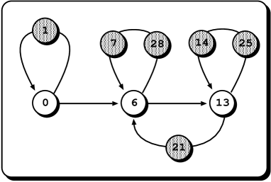
Figure 2: Node dependencies for the completed graph.

In general, a set of mutually dependent subgoals forms a Strongly Connected Component (or SCC) [51]. Clearly, we can only complete SCCs together. We will usually represent an SCC through the oldest generator. More precisely, the youngest generator node which does not depend on older generators is called the leader node. A leader node is also the oldest node for its SCC, and defines the current completion point.

XSB uses a stack of generators to detect completion points [42]. Each time a new generator is introduced it becomes the current leader node. Each time a new consumer is introduced one verifies if it is for an older generator node ${\mathcal{}G}$. If so, ${\mathcal{}G}$’s leader node becomes the current leader node. Unfortunately, this algorithm does not scale well for parallel execution, which is not easily representable with a single stack.

2.4 Scheduling

At several points we had to choose between continuing forward execution, backtracking to interior nodes, returning answers to consumer nodes, or performing completion. Ideally, we would like to run these operations in parallel. In a sequential system, the decision on which operation to perform is crucial to system performance and is determined by the scheduling strategy. Different scheduling strategies may have a significant impact on performance, and may lead to different order of answers. YapTab implements two different scheduling strategies, batched and local [14]. YapTab’s default scheduling strategy is batched.

Batched scheduling is the strategy we followed in the example: it favors forward execution first, backtracking to interior nodes next, and returning answers or completion last. It thus tries to delay the need to move around the search tree by batching the return of answers. When new answers are found for a particular tabled subgoal, they are added to the table space and the evaluation continues until it resolves all program clauses for the subgoal in hand.

Batched scheduling runs all interior nodes before restarting the consumers. In the worst case, this strategy may result in creating a complex graph of interdependent consumers. Local scheduling is an alternative tabling scheduling strategy that tries to evaluate subgoals as independently as possible, by executing one SCC at a time. Answers are only returned to the leader’s calling environment when its SCC is completely evaluated.

3 The Sequential Tabling Engine

We next give a brief introduction to the implementation of YapTab. Throughout, we focus on support for the parallel execution of definite programs.

The YapTab design is WAM based, as is the SLG-WAM. Yap data structures’ are very close to the WAM’s [56]: there is a local stack, storing both choice points and environment frames; a global stack, storing compound terms and variables; a code space area, storing code and the internal database; a trail; and a auxiliary stack. To support the SLG-WAM we must extend the WAM with a new data area, the table space; a new set of registers, the freeze registers; an extension of the standard trail, the forward trail. We must support four new operations: tabled subgoal call, new answer, answer resolution, and completion. Last, we must support one or several scheduling strategies.

We reconsidered decisions in the original SLG-WAM that can be a potential source of parallel overheads. Namely, we argue that the stack based completion detection mechanism used in the SLG-WAM is not suitable to a parallel implementation. The SLG-WAM considers that the control of leader detection and scheduling of unconsumed answers should be done at the level of the data structures corresponding to first calls to tabled subgoals, and it does so by associating completion frames to generator nodes. On the other hand, YapTab considers that such control should be performed through the data structures corresponding to variant calls to tabled subgoals, and thus it associates a new data structure, the dependency frame, to consumer nodes. We believe that managing dependencies at the level of the consumer nodes is a more intuitive approach that we can take advantage of.

The introduction of this new data structure allows us to reduce the number of extra fields in tabled choice points and to eliminate the need for a separate completion stack. Furthermore, allocating the data structure in a separate area simplifies the implementation of parallelism. We next review the main data structures and algorithms of the YapTab design. A more detailed description is given in [36].

3.1 Table Space

The table space can be accessed in different ways: to look up if a subgoal is in the table, and if not insert it; to verify whether a newly found answer is already in the table, and if not insert it; to pick up answers to consumer nodes; and to mark subgoals as completed. Hence, a correct design of the algorithms to access and manipulate the table data is a critical issue to obtain an efficient tabling system implementation.

Our implementation of tables uses tries as proposed by Ramakrishnan et al. [33]. Tries provide complete discrimination for terms and permit lookup and possibly insertion to be performed in a single pass through a term. In section 5.2 we discuss how OPTYap supports concurrent access to tries.

Figure 3 shows the completed table for the query shown in Figure 1. Table lookup starts from the table entry data structure. Each table predicate has one such structure, which is allocated at compilation time. A pointer to the table entry can thus be included in the compiled code. Calls to the predicate will always access the table starting from this point.

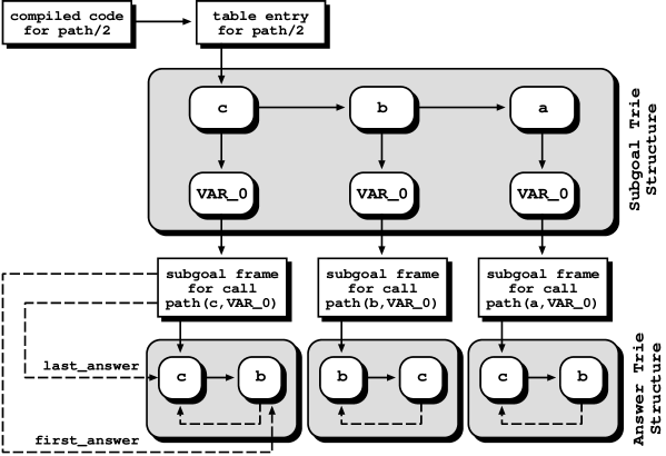
Figure 3: Using tries to organize the table space.

The table entry points to a tree of trie nodes, the subgoal trie structure. More precisely, each different call to path/2 corresponds to a unique path through the subgoal trie structure. Such a path always starts from the table entry, follows a sequence of subgoal trie data units, the subgoal trie nodes, and terminates at a leaf data structure, the subgoal frame.

Each subgoal trie node represents a binding for an argument or sub-argument of the subgoal. In the example, we have three possible bindings for the first argument, X=c, X=b, and X=a. Each binding stores two pointers: one to be followed if the argument matches the binding, the other to be followed otherwise.

We often have to search through a chain of sibling nodes that represent alternative paths, e.g., in the query path(a,Z) we have to search through nodes X=c and X=b until finding node X=a. By default, this search is done sequentially. When the chain becomes larger then a threshold value, we dynamically index the nodes through a hash table to provide direct node access and therefore optimize the search.

Each subgoal frame stores information about the subgoal, namely an entry point to its answer trie structure. Each unique path through the answer trie data units, the answer trie nodes, corresponds to a different answer to the entry subgoal. All answer leave nodes are inserted in a linked list: the subgoal trie points at the first and last entry in this list. Leaves’ answer nodes are chained together in insertion time order, so that we can recover answers in the same order they were inserted. A consumer node thus needs only to point at the leaf node for its last consumed answer, and consumes more answers just by following the chain of leaves.

3.2 Generator and Consumer Nodes

Generator and consumer nodes correspond, respectively, to first and variant calls to tabled subgoals, while interior nodes correspond to normal, not tabled, subgoals. Interior nodes are implemented at the engine level as WAM choice points. To implement generator nodes we extended the WAM choice points with a pointer to the corresponding subgoal frame. To implement consumer nodes we use the notion of dependency frame. Dependency frames will be stored in a proper space, the dependency space. Figure 4 illustrates how generator and consumer nodes interact with the table and dependency spaces. As we shall see in section 5.3, having a separate dependency space is quite useful for our copying-based implementation, although dependency frames could be stored together with the corresponding choice point in the sequential implementation. All dependency frames are linked together to form a dependency list of consumer nodes. Additionally, dependency frames store information about the last consumed answer for the correspondent consumer node; and information for detecting completion points, as we discuss next.

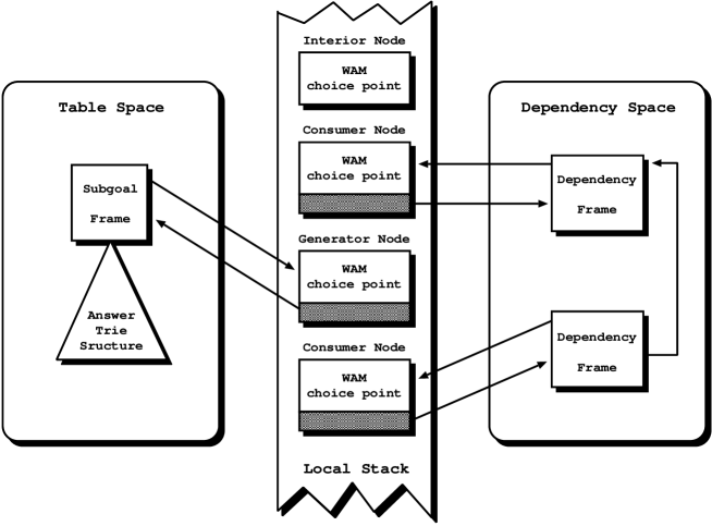
Figure 4: The nodes and their relationship with the table and dependency spaces.

3.3 Leader Nodes

We need to perform completion in order to recover space and in order to determine negative loops between subgoals in programs with negation. In this work we focus on positive programs only, so our goal will be to recover space. Unfortunately, as an artifact of the SLG-WAM, it can happen that the stack segments for a SCC ${\mathcal{}S}$ remain within the stack segments for another SCC ${\mathcal{}S^{\prime}}$. In such cases, ${\mathcal{}S}$ cannot be recovered in advance when completed, and thus, recovering its space must be delayed until ${\mathcal{}S^{\prime}}$ also completes. To approximate SCCs in a stack-based implementation, Sagonas [41] denotes a set of SCCs whose space must be recovered together as an Approximate SCC or ASCC. For simplicity, in the following we will use the SCC notation to refer to both ASCCs and SCCs.

The completion operation takes place when we backtrack to a generator node that (i) has exhausted all its alternatives and that (ii) is as a leader node (remember that the youngest generator node which does not depend on older generators is called a leader node). We designed novel algorithms to quickly determine whether a generator node is a leader node. The key idea in our algorithms is that each dependency frame holds a pointer to the resulting leader node of the SCC that includes the correspondent consumer node. Using the leader node pointer from the dependency frames, a generator node can quickly determine whether it is a leader node. More precisely, in our algorithm, a generator ${\mathcal{}L}$ is a leader node when either (a) ${\mathcal{}L}$ is the youngest tabled node, or (b) the youngest consumer that says ${\mathcal{}L}$ is the leader.

Our algorithm thus requires computing leader node information whenever creating a new consumer node ${\mathcal{}C}$. We proceed as follows. First, we hypothesize that the leader node is ${\mathcal{}C}$’s generator, say ${\mathcal{}G}$. Next, for all consumer nodes older than ${\mathcal{}C}$ and younger than ${\mathcal{}G}$, we check whether they depend on an older generator node. Consider that there is at least one such node and that the oldest of these nodes is ${\mathcal{}G^{\prime}}$. If so then ${\mathcal{}G^{\prime}}$ is the leader node. Otherwise, our hypothesis was correct and the leader node is indeed ${\mathcal{}G}$. Leader node information is implemented as a pointer to the choice point of the newly computed leader node.

Figure 5 uses the example from Figure 1 to illustrate the leader node algorithm. For compactness, the figure presents calls to path(a,Z), path(b,Z), path(c,Z) and arc(a,Z), as pa, pb, pc, and aa, respectively. Figure 5(a) shows the initial configuration. The generator node ${\mathcal{}N}_{0}$ is the current leader node because it is the only subgoal. Figure 5(b) shows the dependency graph after creating node ${\mathcal{}N}_{2}$. First, we called a variant of path(a,Z), and allocated the corresponding dependency frame. ${\mathcal{}N}_{0}$ is the generator node for the variant call path(a,Z), ${\mathcal{}N}_{0}$ is the leader node for ${\mathcal{}N}_{1}$’s. ${\mathcal{}N}_{1}$ then suspended, we backtracked to ${\mathcal{}N}_{0}$ and called arc(a,Z). As arc(a,Z) is not tabled, we had to allocate an interior node for ${\mathcal{}N}_{2}$.

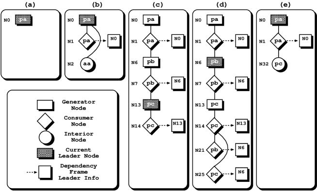
Figure 5: Spotting the current leader node.

Figure 5(c) shows the graph after we created node ${\mathcal{}N}_{14}$. We have already created first and variant calls to subgoals path(b,Z) and path(c,Z). Two new dependency frames were allocated and initialized. We thus have three SCCs on stack: one per generator. The youngest SCC on stack is for subgoal path(c,Z). As a result, the current leader node for the new set of nodes becomes ${\mathcal{}N}_{13}$. This is the one referred in the youngest dependency frame.

Figure 5(d) shows the interesting case where tabled nodes exist between a consumer and its generator. In the example, consumer node ${\mathcal{}N}_{21}$, has two consumers, ${\mathcal{}N}_{7}$ and ${\mathcal{}N}_{14}$, separating it from its generator, ${\mathcal{}N}_{6}$. As both consumers do not depend on nodes older than ${\mathcal{}N}_{6}$, the leader node for ${\mathcal{}N}_{21}$ is still ${\mathcal{}N}_{6}$, and ${\mathcal{}N}_{6}$ becomes the current leader node. This situation represents the point at which subgoal path(c,Z) starts depending on subgoal path(b,Z) and their SCCs are merged together. Next, we allocated consumer node ${\mathcal{}N}_{25}$. Nodes ${\mathcal{}N}_{14}$ and ${\mathcal{}N}_{21}$ are between ${\mathcal{}N}_{25}$ and the generator ${\mathcal{}N}_{13}$. Our algorithm says that since ${\mathcal{}N}_{21}$ depends on an older generator node, ${\mathcal{}N}_{6}$, the leader node information for ${\mathcal{}N}_{25}$ is also ${\mathcal{}N}_{6}$. As a result, ${\mathcal{}N}_{6}$ remains the current leader node.

Finally, Figure 5(e) shows the point after the subgoals path(b,Z) and path(c,Z) have completed and the segments belonging to their SCC have been released. The computation switches back to ${\mathcal{}N}_{1}$, consumes the next answer and calls path(c,Z). At this point, path(c,Z) is already completed, and thus we can avoid consumer node allocation and instead perform what is called the completed table optimization [42]. This optimization allocates a node, similar to an interior node, that will consume the set of found answers executing compiled code directly from the trie data structure associated with the completed subgoal [33].

3.4 Completion and Answer Resolution

After backtracking to a leader node, we must check whether all younger consumer nodes have consumed all their answers. To do so, we walk the chain of dependency frames looking for a frame which has not yet consumed all the generated answers. If there is such a frame, we should resume the computation of the corresponding consumer node. We do this by restoring the stack pointers and backtracking to the node. Otherwise, we can perform completion. This includes (i) marking as complete all the subgoals in the SCC; (ii) deallocating all younger dependency frames; and (iii) backtracking to the previous node to continue the execution.

Backtracking to a consumer node results in executing the answer resolution operation. The operation first checks the table space for unconsumed answers. If there are new answers, it loads the next available answer and proceeds. Otherwise, it backtracks again. If this is the first time that backtracking from that consumer node takes place, then it is performed as usual. Otherwise, we know that the computation has been resumed from an older generator node ${\mathcal{}G}$ during an unsuccessful completion operation. Therefore, backtracking must be done to the next consumer node that has unconsumed answers and that is younger than ${\mathcal{}G}$. If no such consumer node can be found, backtracking must be done to the generator node ${\mathcal{}G}$.

The process of resuming a consumer node, consuming the available set of answers, suspending and then resuming another consumer node can be seen as an iterative process which repeats until a fixpoint is reached. This fixpoint is reached when the SCC is completely evaluated.

4 Or-Parallelism within Tabling

The first step in our research was to design a model that would allow concurrent execution of all available alternatives, be they from generator, consumer or interior nodes. We researched two designs: the TOP (Tabling within Or Parallelism) model and the OPT (Or-Parallelism within Tabling) model.

Parallelism in the TOP model is supported by considering that a parallel evaluation is performed by a set of independent WAM engines, each managing an unique branch of the search tree at a time. These engines are extended to include direct support to the basic table access operations, that allow the insertion of new subgoals and answers. When exploiting parallelism, some branches may be suspended. Generator and interior nodes suspend alternatives because we do not have enough processors to exploit them all. Consumer nodes may also suspend because they are waiting for more answers. Workers move in the search tree, looking for points where they can exploit parallelism.

Parallel evaluation in the OPT model is done by a set of independent tabling engines that may share different common branches of the search tree during execution. Each worker can be considered a sequential tabling engine that fully implements the tabling operations: access the table space to insert new subgoals or answers; allocate data structures for the different types of nodes; suspend tabled subgoals; resume subcomputations to consume newly found answers; and complete private (not shared) subgoals. As most of the computation time is spent in exploiting the search tree involved in a tabled evaluation, we can say that tabling is the base component of the system.

The or-parallel component of the system is triggered to allow synchronized access to the shared parts of the execution tree, in order to get new work when a worker runs out of alternatives to exploit, and to perform completion of shared subgoals. Unexploited alternatives should be made available for parallel execution, regardless of whether they originate from generator, consumer or interior nodes. From the viewpoint of SLG resolution, the OPT computational model generalizes the Warren’s multi-sequential engine framework for the exploitation of or-parallelism. Or-parallelism stems from having several engines that implement SLG resolution, instead of implementing Prolog’s SLD resolution.

We have already seen that the SLG-WAM presents several opportunities for parallelism. Figure 6 illustrates how this parallelism can be specifically exploited in the OPT model. The example assumes two workers, ${{\mathcal{}W}_{1}}$ and ${{\mathcal{}W}_{2}}$, and the program code and query goal from Figure 1. For simplicity, we use the same abbreviation introduced in Figure 5 to denote the subgoals.

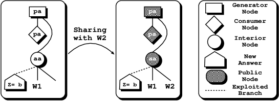
Figure 6: Exploiting parallelism in the OPT model.

Consider that worker ${\mathcal{}W}_{1}$ starts the evaluation. It first allocates a generator and a consumer node for tabled subgoal path(a,Z). Because there are no available answers for path(a,Z), it backtracks. The next alternative leads to a non-tabled subgoal arc(a,Z) for which we create an interior node. The first alternative for arc(a,Z) succeeds with the answer Z=b. The worker inserts the newly found answer in the table and starts exploiting the next alternative for arc(a,Z). This is shown in the left sub-figure. At this point, worker ${\mathcal{}W}_{2}$ requests for work. Assume that worker ${\mathcal{}W}_{1}$ decides to share all of its private nodes. The two workers will share three nodes: the generator and consumer nodes for path(a,Z), and the interior node for arc(a,Z). Worker ${\mathcal{}W}_{2}$ takes the next unexploited alternative of arc(a,Z) and from now on, either worker can find further answers for path(a,Z) or resume the shared consumer node.

The OPT model offers two important advantages over the TOP model. First, OPT reduces to a minimum the overlap between or-parallelism and tabling. Namely, as the example shows, in OPT it is straightforward to make nodes public only when we want to share them. This is very important because execution of private nodes is almost as fast as sequential execution. Second, OPT enables different data structures for or-parallelism and for tabling. For instance, one can use the SLG-WAM for tabling, and environment copying or binding arrays for or-parallelism.

The question now is whether we can achieve an implementation of the OPT model, and whether that implementation is efficient. We implemented OPTYap in order to answer this question. In OPTYap, tabling is implemented by freezing the whole stacks when a consumer blocks. Or-parallelism is implemented through copying of stacks. More precisely, we optimize copying by using incremental copying, where workers only copy the differences between their stacks. We adopted this framework because environment copying and the SLG-WAM are, respectively, two of the most successful or-parallel and tabling engines. In our case, we already had the experience of implementing environment copying in the Yap Prolog, the YapOr system, with excellent performance results [38]. Adopting YapOr for the or-parallel component of the combined system was therefore our first choice.

Regarding the tabling component, an alternative to freezing the stacks is copying them to a separate storage as in CHAT [12]. We found two major problems with CHAT. First, to take best advantage of CHAT we need to have separate environment and choice point stacks, but Yap has an integrated local stack. Second, and more importantly, we believe that CHAT is less suitable than the SLG-WAM to an efficient extension to or-parallelism because of its incremental completion technique. CHAT implements incremental completion through an incremental copying mechanism that saves intermediate states of the execution stacks up to the nearest generator node. This works fine for sequential tabling, because leader nodes are always generator nodes. However, as we will see, for parallel tabling this does not hold because any public node can be a potential leader node. To preserve incremental completion efficiency in a parallel tabling environment, incremental saving should be performed up to the parent node, as potentially it can be a leader node. Obviously, this node-to-node segmentation of the incremental saving technique will degrade the efficiency of any parallel system.

5 The Or-Parallel Tabling Engine

The OPT model requires changes to both the initial designs for parallelism and tabling. As we enumerated next, support or-parallelism plus tabling requires changes to memory allocation, table access, the completion algorithm. We must further ensure that environment copying and tabling suspension do not interfere. Or-parallelism issues refer to scheduling and to speculative work. In more detail:

1. We must support parallel memory allocation and deallocation of the several data structures we use. Fortunately, most of our data structures are fixed-sized and parallel memory allocation can be implemented efficiently.

2. We must allow for several workers to concurrently read and update the table. To do so workers need to be able to lock the table. As we shall see finer locking allows for more parallelism, but coarser locking has less overheads.

3. OPTYap uses the copying model, where workers do not see the whole search tree, but instead only the branches corresponding to their current SLG-WAM. It is thus possible that a generator may not be in the stacks for a consumer (and vice-versa). We show that one can generalize the concept of leader node for such cases, and that such a generalization still gives a conservative approximation for a SCC. Completion can thus be performed when we are the last worker backtracking to the generalized leader nodes, and there is no more work below. The first condition can be easily checked through the or-parallel machinery. The second condition uses the sequential tabling machinery.

4. Or-parallelism and tabling are not strictly orthogonal. More precisely, naively sharing or-parallel work might result in overwriting suspended stacks. Several approaches may be used to tackle this problem, we have proposed and implemented a suspension mechanism that gives maximum scheduling flexibility.

5. Scheduling or-parallel work in our system is based on the Muse scheduler [1]. Intuitively this corresponds to a form of hierarchical scheduling, where we favor tabled scheduling operations, and resort to the more expensive or-parallel scheduling when no tabling operations are available. Other approaches are possible, but this one has served OPTYap well so far. We also discuss how moving around the shared parts of the search tree changes in the presence of parallelism.

6. Last, we briefly discuss pruning issues. Although pruning in the presence of tabling is a complex issue [16, 25], we still should execute correctly for non-tabled regions of the search tree (interior nodes).

We next discuss these issues in some detail, presenting the general execution framework.

5.1 Memory Organization

In OPTYap, memory is divided into a global addressing space and a collection of local spaces, as illustrated in Figure 7. The global space includes the code area and a parallel data area that consists of all the data structures required to support concurrent execution. Each local space represents one system worker and it contains the four WAM execution stacks inherited from Yap: global stack, local stack, trail, and auxiliary stack.

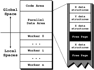
Figure 7: Memory organization in OPTYap.

The parallel data area includes the table and dependency spaces inherited from YapTab, and the or-frame space [1] inherited from YapOr to synchronize access to shared nodes. Additionally, we have an extra data structure to preserve the stacks of suspended SCCs (further details in section 5.4). Remember that we use specific extra fields in the choice points to access the data structures in the parallel data area. When sharing work, the execution stacks of the sharing worker are copied from its local space to the local space of the requesting worker. The data structures from the parallel data area associated with the shared stacks are automatically inherited by the requesting worker in the copied choice points.

The efficiency of a parallel system largely depends on how concurrent handling of shared data is achieved and synchronized. Page faults and memory cache misses are a major source of overhead regarding data access or update in parallel systems. OPTYap tries to avoid these overheads by adopting a page-based organization scheme to split memory among different data structures, in a way similar to Bonwick’s Slab memory allocator [6]. Each memory page of the parallel data area only contains data structures of the same type. Whenever a new request for a data structure of type ${\mathcal{}T}$ appears, the next available structure on one of the ${\mathcal{}T}$ pages is returned. If there are no available structures in any ${\mathcal{}T}$ page, then one of the free pages is made to be of type ${\mathcal{}T}$. A page is freed when all its data structures are released. A free page can be immediately reassigned to a different structure type.

5.2 Concurrent Table Access

Our experience showed that the table space is the major data area open to concurrent access operations in a parallel tabling environment. To maximize parallelism, whilst minimizing overheads, accessing and updating the table space must be carefully controlled. Reader/writer locks are the ideal implementation scheme for this purpose. In a nutshell, we can say that there are two critical issues that determine the efficiency of a locking scheme for the table. One is the lock duration, that is, the amount of time a data structure is locked. The other is the lock grain, that is, the amount of data structures that are protected through a single lock request. It is the balance between lock duration and lock grain that compromises the efficiency of different table locking approaches. For instance, if the lock scheme is short duration or fine grained, then inserting many trie nodes in sequence, corresponding to a long trie path, may result in a large number of lock requests. On the other hand, if the lock scheme is long duration or coarse grain, then going through a trie path without extending or updating its trie structure, may unnecessarily lock data and prevent possible concurrent access by others.

Unfortunately, it is impossible beforehand to know which locking scheme would be optimal. Therefore, in OPTYap we experimented with four alternative locking schemes to deal with concurrent accesses to the table space data structures, the Table Lock at Entry Level scheme, TLEL, the Table Lock at Node Level scheme, TLNL, the Table Lock at Write Level scheme, TLWL, and the Table Lock at Write Level - Allocate Before Check scheme, TLWL-ABC.

The TLEL scheme essentially allows a single writer per subgoal trie structure and a single writer per answer trie structure. The main drawback of TLEL is the contention resulting from long lock duration. The TLNL enables a single writer per chain of sibling nodes that represent alternative paths from a common parent node. The TLWL scheme is similar to TLNL in that it enables a single writer per chain of sibling nodes that represent alternative paths to a common parent node. However, in TLWL, the common parent node is only locked when writing to the table is likely. TLWL also avoids the TLNL memory usage problem by replacing trie node lock fields with a global array of lock entries. Last, the TLWL-ABC scheme anticipates the allocation and initialization of nodes that are likely to be inserted in the table space before locking.

Through experimentation, we observed that the locking schemes, TLWL and TLWL-ABC, present the best speedup ratios and they are the only schemes showing scalability. Since none of these two schemes clearly outperform the other, we assumed TLWL as the default. The observed slowdown with higher number of workers for TLEL and TLNL schemes is mainly due to their locking of the table space even when writing is not likely. In particular, for repeated answers they pay the cost of performing locking operations without inserting any new trie node. For these schemes the number of potential contention points is proportional to the number of answers found during execution, being they unique or redundant.

5.3 Leader Nodes

Or-parallel systems execute alternatives early. As a result, different workers may execute the generator and the consumer subgoals. In fact, it is possible that generators will execute earlier, and in a different branch than in sequential execution. As Figure 8 shows, this may induce complex dependencies between workers, therefore requiring a more elaborate completion algorithm that may involve branches from several workers.

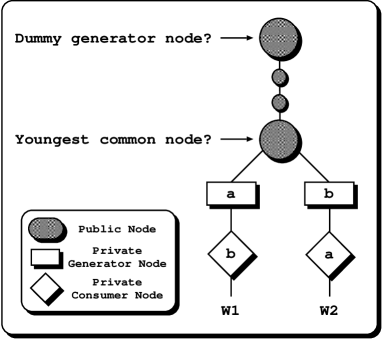
Figure 8: At which node should we check for completion?

In this example, worker ${\mathcal{}W}_{1}$ takes the leftmost alternative while worker ${\mathcal{}W}_{2}$ takes the rightmost from the youngest common node. While exploiting their alternatives, ${\mathcal{}W}_{1}$ calls a tabled subgoal a and ${\mathcal{}W}_{2}$ calls a tabled subgoal b. As this is the first call to both subgoals, a generator node is stored for each one. Next, each worker calls the tabled subgoal firstly called by the other, and two consumer nodes, one per worker, are therefore allocated. At this point both workers hold a consumer node while not having the corresponding generator node in their branches. Conversely, the owner of each generator node has consumer nodes being executed by a different worker. The question is where should we check for completion? Intuitively, we would like to choose a node that is common to both branches and the youngest common node seems the better choice. But that node is not a generator node!

We could avoid this problem by disallowing consumer nodes for generator nodes on other branches. Unfortunately, such a solution would severely restrict parallelism. Our solution was therefore to allow completion at all kind of public nodes.

To clarify these new situations we introduce a new concept, the Generator Dependency Node (or GDN). Its purpose is to signal the nodes that are candidates to be leader nodes, therefore representing a similar role as that of the generator nodes for sequential tabling. A GDN is calculated whenever a new consumer node, say ${\mathcal{}C}$, is created. We define the GDN ${\mathcal{}D}$ for a consumer node ${\mathcal{}C}$ with generator $\mathcal{}G$ to be the youngest node on ${\mathcal{}C}$’s current branch that is an ancestor of ${\mathcal{}G}$. Obviously, if ${\mathcal{}G}$ belongs to the current branch of ${\mathcal{}C}$ then ${\mathcal{}G}$ must be the GDN. Thus GDN reduces to leader node for sequential computations. On the other hand, if the worker allocating ${\mathcal{}C}$ is not the one that allocated ${\mathcal{}G}$ then the youngest node ${\mathcal{}D}$ is a public node, but not necessarily ${\mathcal{}G}$. Figure 9 presents three different situations that better illustrate the GDN concept. ${\mathcal{}W_{G}}$ is always the worker that allocated the generator node ${\mathcal{}G}$, and ${\mathcal{}W_{C}}$ is the worker that is allocating a consumer node ${\mathcal{}C}$.

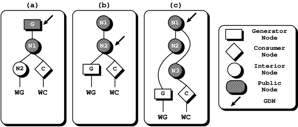
Figure 9: Spotting the generator dependency node.

In situation (a), the generator node ${\mathcal{}G}$ is on the branch of the consumer node ${\mathcal{}C}$, and thus, ${\mathcal{}G}$ is the GDN. In situation (b), nodes ${\mathcal{}N}_{1}$ and ${\mathcal{}N}_{2}$ are on the branch of ${\mathcal{}C}$ and both contain a branch leading to the generator ${\mathcal{}G}$. As ${\mathcal{}N}_{2}$ is the youngest node of the two, it is the GDN. Situation (c) differs from (b) in that the public nodes represent more than one branch and, in this case, are interleaved in the physical stack. In this situation, ${\mathcal{}N}_{1}$ is the unique node that belongs to ${\mathcal{}C}$’s branch and that also contains ${\mathcal{}G}$ in a branch below. ${\mathcal{}N}_{2}$ contains ${\mathcal{}G}$ in a branch below, but it is not on ${\mathcal{}C}$’s branch, while ${\mathcal{}N}_{3}$ is on ${\mathcal{}C}$’s branch, but it does not contain ${\mathcal{}G}$ in a branch below. Therefore, ${\mathcal{}N}_{1}$ is the GDN. Notice that in both cases (b) and (c) the GDN can be a generator, a consumer or an interior node.

The procedure that computes the leader node information when allocating a new dependency frame now relies on the GDN concept. Remember that it is through this information that a node can determine whether it is a leader node. The main difference from the sequential algorithm is that now we first hypothesize that the leader node for the consumer node in hand is its GDN, and not its generator node. Then, we check the consumer nodes younger than the newly found GDN for an older dependency. Note that as soon as an older dependency ${\mathcal{}D}$ is found in a consumer node ${\mathcal{}C^{\prime}}$, the remaining consumer nodes, older than ${\mathcal{}C^{\prime}}$ but younger than the GDN, do not need to be checked. This is safe because the previous computation of the leader node information for the consumer node ${\mathcal{}C^{\prime}}$ already represents the oldest dependency that includes the remaining consumer nodes. We next give an argument on the correctness of the algorithm.

Consider a consumer node with GDN ${\mathcal{}G}$ and assume that its leader node ${\mathcal{}D}$ is found in the dependency frame for consumer node ${\mathcal{}C}$. Now hypothesize that there is a consumer node ${\mathcal{}N}$ younger than ${\mathcal{}G}$ with a reference ${\mathcal{}D^{\prime}}$ older than ${\mathcal{}D}$. Therefore, when previously computing the leader node for ${\mathcal{}C}$ one of the following situations occurred: (i) ${\mathcal{}D}$ is the GDN for ${\mathcal{}C}$ or (ii) ${\mathcal{}D}$ was found in a dependency frame for a consumer node ${\mathcal{}C^{\prime}}$. Situation (i) is not possible because ${\mathcal{}N}$ is younger than ${\mathcal{}D}$ and it holds a reference older than ${\mathcal{}D}$. Regarding situation (ii), ${\mathcal{}C^{\prime}}$ is necessarily younger than ${\mathcal{}N}$ as otherwise the reference found for ${\mathcal{}C}$ had been ${\mathcal{}D^{\prime}}$. By recursively applying the previous argument to the computation of the leader node for ${\mathcal{}C^{\prime}}$ we conclude that our initial hypothesis cannot hold because the number of nodes between ${\mathcal{}C}$ and ${\mathcal{}N}$ is finite.

With this scheme, concurrency is not a problem. Each worker views its own leader node independently from the execution being done by others. A new consumer node is always a private node and a new dependency frame is always the youngest dependency frame for a worker. The leader information stored in a dependency frame denotes the resulting leader node at the time the correspondent consumer node was allocated. Thus, after computing such information it remains unchanged. If when allocating a new consumer node the leader changes, the new leader information is only stored in the dependency frame for the new consumer, therefore not influencing others. Observe, for example, the situation from Figure 10. Two workers, ${\mathcal{}W}_{1}$ and ${\mathcal{}W}_{2}$, exploiting different alternatives from a common public node, ${\mathcal{}N}_{4}$, are allocating new private consumer nodes. They compute the leader node information for the new dependency frames without requiring any explicit communication between both and without requiring any synchronization if consulting the common dependency frame for node ${\mathcal{}N}_{4}$. The resulting dependency chain for each worker is illustrated on each side of the figure. Note that the dependency frame for consumer node ${\mathcal{}N}_{4}$ is common to both workers. It is illustrated twice only for simplicity.

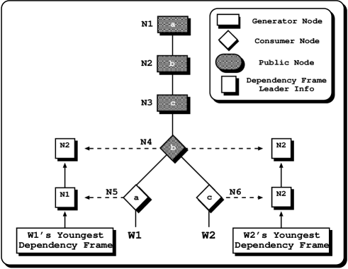
Figure 10: Dependency frames in the parallel environment.

Within this scenario, worker ${\mathcal{}W}_{1}$ will check for completion at node ${\mathcal{}N}_{1}$, its current leader node, and worker ${\mathcal{}W}_{2}$ will check for completion at node ${\mathcal{}N}_{2}$. Obviously, ${\mathcal{}W}_{2}$ cannot perform completion when reaching ${\mathcal{}N}_{2}$. If ${\mathcal{}W}_{1}$ finds new answers for subgoal c, they should be consumed in node ${\mathcal{}N}_{6}$. Moreover, as ${\mathcal{}W}_{1}$ has a dependency for an older node, ${\mathcal{}N}_{1}$, the SCCs from both workers should only be completed together at node ${\mathcal{}N}_{1}$. However, ${\mathcal{}W}_{1}$ can allocate another consumer node that changes its current leader node. Therefore, ${\mathcal{}W}_{2}$ cannot know beforehand the leader where both SCCs should be completed. Determining the leader node where several dependent SCCs from different workers may be completed together is the problem that we address next.

5.4 SCC Suspension

Different paths may be followed when a worker ${\mathcal{}W}$ reaches a leader node for a SCC ${\mathcal{}S}$. The simplest case is when the node is private. In this case, we proceed as for sequential tabling. Otherwise, the node is public, and other workers can still influence ${\mathcal{}S}$. For instance, these workers may find new answers for a consumer node in ${\mathcal{}S}$, in which case the consumer must be resumed to consume the new answers. Clearly, in such cases, ${\mathcal{}W}$ should not complete. On the other hand, ${\mathcal{}W}$ has tried all available alternatives and would like to move anywhere in the tree, say to node ${\mathcal{}N}$, to try other work. According to the copying model we use for or-parallelism, we should backtrack to the youngest node common to ${\mathcal{}N}$’s branch, that is, we should reset our stacks to the values of the common node. According to the freezing model that we use for tabling, we cannot recover the current consumers because they are frozen. We thus have a contradiction.

Note that this is the only case where or-parallelism and tabling conflict. One solution would be to disallow movement in this case. Unfortunately, we would again severely restrict parallelism. As a result, in order to allow ${\mathcal{}W}$ to continue execution it becomes necessary to suspend the SCC at hand. Suspending a SCC includes saving the SCC’s stacks to a proper space, leaving in the leader node a reference to the suspended SCC. These suspended computations are considered again when the remaining workers do completion.

In order to find out which suspended SCCs need to be resumed, each worker maintains a list of nodes with suspended SCCs. The last worker backtracking from a public node ${\mathcal{}N}$ checks if it holds references to suspended SCCs. If so, then ${\mathcal{}N}$ is included in the worker’s list of nodes with suspended SCCs (the nodes are linked in stack order). If the node already belongs to other worker’s list, it is not collected.

A suspended SCC should be resumed if it contains consumer nodes with unconsumed answers. To resume a suspended SCC a worker needs to copy the saved stacks to the correct position in its own stacks, and thus, it has to suspend its current SCC first. Figure 11 illustrates the management of suspended SCCs when searching for SCCs to resume. It considers a worker ${\mathcal{}W}$, positioned in the leader node ${\mathcal{}N}_{1}$ of its current SCC ${\mathcal{}S}_{1}$. ${\mathcal{}W}$ consults its list of nodes with suspended SCCs, and starts checking the suspended SCC ${\mathcal{}S}_{4}$ for unconsumed answers. Assuming that ${\mathcal{}S}_{4}$ does not contain unconsumed answers, the search continues in the next node in the list. Here, suppose that SCC ${\mathcal{}S}_{2}$ does not have consumer nodes with unconsumed answers, but SCC ${\mathcal{}S}_{3}$ does. The current SCC ${\mathcal{}S}_{1}$ is then suspended, and only then ${\mathcal{}S}_{3}$ resumed.

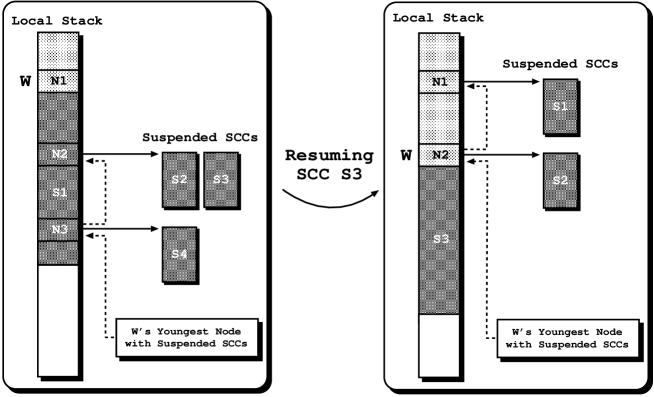
Figure 11: Resuming a suspended SCC.

Notice that node ${\mathcal{}N}_{3}$ was removed from ${\mathcal{}W}$’s list of suspended SCCs because ${\mathcal{}S}_{3}$ may not include ${\mathcal{}N}_{3}$ in its stack segments. For simplicity and efficiency, instead of checking ${\mathcal{}S}_{3}$’s segments, we simply remove ${\mathcal{}N}_{3}$’s from ${\mathcal{}W}$’s list. Note that this is a safe decision as a SCC only depends from branches below the leader node. Thus, if ${\mathcal{}S}_{3}$ does not include ${\mathcal{}N}_{3}$ then no new answers can be found for ${\mathcal{}S}_{4}$’s consumer nodes. Otherwise, if this is not the case then ${\mathcal{}W}$ or other workers can eventually be scheduled to a node held by ${\mathcal{}S}_{4}$ and find new answers for at least one of its consumer nodes. In this case, when failing, these workers will necessarily backtrack through ${\mathcal{}N}_{3}$, ${\mathcal{}S}_{4}$’s leader. Therefore, the last worker backtracking from ${\mathcal{}N}_{3}$ will collect it for its own list, which allows ${\mathcal{}S}_{4}$ to be later resumed when executing completion in an older leader node.

5.5 The Flow of Control

Actual execution control of a parallel tabled evaluation mainly flows through four procedures. The process of completely evaluating SCCs is accomplished by the completion() and answer_resolution() procedures, while parallel synchronization is achieved by the getwork() and scheduler() procedures. Here we focus on the execution in engine mode, that is on the completion(), answer_resolution() and getwork() procedures, and leave scheduling for the following section. Figure 12 presents a general overview of how control flows between the three procedures and how it flows within each procedure.

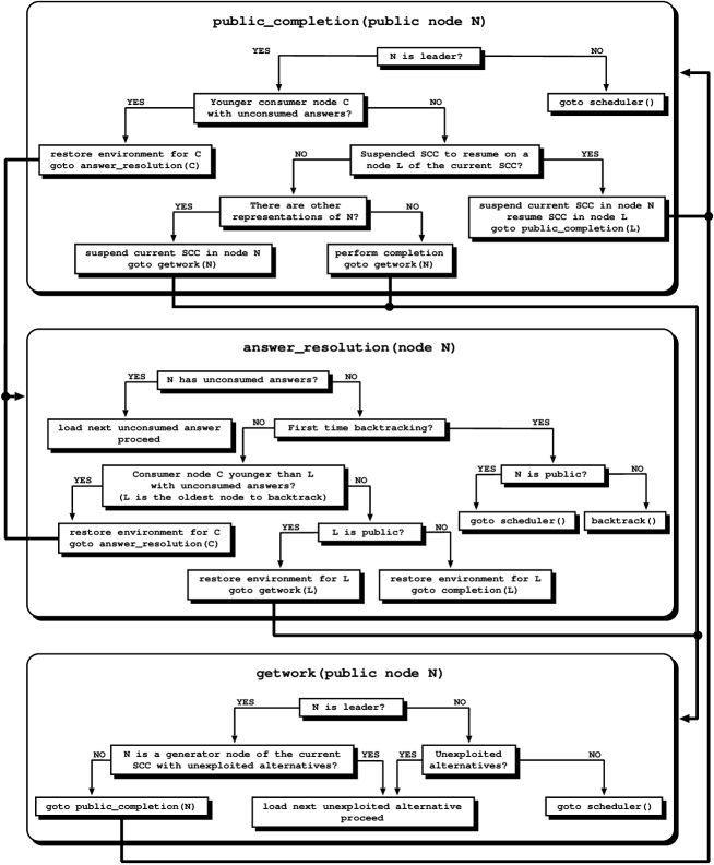
Figure 12: The flow of control in a parallel tabled evaluation.

A novel completion procedure, public_completion(), implements completion detection for public leader nodes. As for private nodes, whenever a public node finds that it is a leader, it starts to check for younger consumer nodes with unconsumed answers. If there is such a node, we resume the computation to it. Otherwise, it checks for suspended SCCs with unconsumed answers. Remember that to resume a suspended SCC a worker needs to suspend its current SCC first.

We thus adopted the strategy of resuming suspended SCCs only when the worker finds itself at a leader node, since this is a decision point where the worker either completes or suspends the current SCC. Hence, if the worker resumes a suspended SCC it does not introduce further dependencies. This is not the case if the worker would resume a suspended SCC ${\mathcal{}R}$ as soon as it reached the node where it had suspended. In that situation, the worker would have to suspend its current SCC ${\mathcal{}S}$, and after resuming ${\mathcal{}R}$ it would probably have to also resume ${\mathcal{}S}$ to continue its execution. A first disadvantage is that the worker would have to make more suspensions and resumptions. Moreover, if we resume earlier, ${\mathcal{}R}$ may include consumer nodes with unconsumed answers that are common with ${\mathcal{}S}$. More importantly, suspending in non-leader nodes leads to further complexity that can be very difficult to manage.

A SCC ${\mathcal{}S}$ is completely evaluated when (i) there are no unconsumed answers in any consumer node belonging to ${\mathcal{}S}$ or in any consumer node within a SCC suspended in a node belonging to ${\mathcal{}S}$; and (ii) there are no other representations of the leader node ${\mathcal{}N}$ in the computational environment, be ${\mathcal{}N}$ represented in the execution stacks of a worker or be ${\mathcal{}N}$ in the suspended stack segments of a SCC. Completing a SCC includes (i) marking all dependent subgoals as complete; (ii) releasing the frames belonging to the complete branches, including the branches in suspended SCCs; (iii) releasing the frozen stacks and the memory space used to hold the stacks from suspended SCCs; and (iv) readjusting the freeze registers and the whole set of stack and frame pointers.

The answer resolution operation for the parallel environment essentially uses the same algorithm as previously described for private nodes (please refer to section 3.4). Initially, the procedure checks for unconsumed answers to be loaded for execution. If we have answers, execution will jump to them. Otherwise, we schedule for a backtracking node. If this is not the first time that backtracking from that consumer node takes place, we know that the computation has been resumed from an older leader node ${\mathcal{}L}$ during an unsuccessful completion operation. ${\mathcal{}L}$ is thus the oldest node to where we can backtrack. Backtracking must be done to the next consumer node that has unconsumed answers and that is younger than ${\mathcal{}L}$. Otherwise, if there are no such consumer nodes, backtracking must be done to ${\mathcal{}L}$.

The getwork() procedure contributes to the progress of a parallel tabled evaluation by moving to effective work. The usual way to execute getwork() is through failure to the youngest public node on the current branch. We can distinguish two main procedures in getwork(). One detects completion points and therefore makes the computation flow to the public_completion() procedure. The other corresponds to or-parallel execution. It synchronizes to check for available alternatives and executes the next one, if any. Otherwise, it invokes the scheduler. A completion point is detected when ${\mathcal{}N}$ is the leader node pointed by the youngest dependency frame. The exception is if ${\mathcal{}N}$ is itself a generator node for a consumer node within the current SCC and it contains unexploited alternatives. In such cases, the current SCC is not fully exploited. Hence, we should exploit first the available alternatives, and only then invoke completion.

5.6 Scheduling Work

Scheduling work is the scheduler’s task. It is about efficiently distributing the available work for exploitation between the running workers. In a parallel tabling environment we have the extra constraint of keeping the correctness of sequential tabling semantics. A worker enters in scheduling mode when it runs out of work and returns to execution whenever a new piece of unexploited work is assigned to it by the scheduler.

The scheduler for the OPTYap engine is mainly based on YapOr’s scheduler. All the scheduler strategies implemented for YapOr were used in OPTYap. However, extensions were introduced in order to preserve the correctness of tabling semantics. These extensions allow support for leader nodes, frozen stack segments, and suspended SCCs. The OPTYap model was designed to enclose the computation within a SCC until the SCC was suspended or completely evaluated. Thus, OPTYap introduces the constraint that the computation cannot flow outside the current SCC, and workers cannot be scheduled to execute at nodes older than their current leader node. Therefore, when scheduling for the nearest node with unexploited alternatives, if it is found that the current leader node is younger than the potential nearest node with unexploited alternatives, then the current leader node is the node scheduled to proceed with the evaluation.

The next case is when the scheduling to determine the nearest node with unexploited alternatives does not return any node to proceed execution. The scheduler then starts searching for busy workers that can be demanded for work. If such a worker ${\mathcal{}B}$ is found, then the requesting worker moves up to the youngest node that is common to ${\mathcal{}B}$, in order to become partially consistent with part of ${\mathcal{}B}$. Otherwise, no busy worker was found, and the scheduler moves the idle worker to a better position in the search tree. Therefore, we can enumerate three different situations for a worker to move up to a node ${\mathcal{}N}$: (i) ${\mathcal{}N}$ is the nearest node with unexploited alternatives; (ii) ${\mathcal{}N}$ is the youngest node common with the busy worker we found; or (iii) ${\mathcal{}N}$ corresponds to a better position in the search tree.

The process of moving up in the search tree from a current node ${\mathcal{}N}_{0}$ to a target node ${\mathcal{}N}_{f}$ is mainly implemented by the move_up_one_node() procedure. This procedure is invoked for each node that has to be traversed until reaching ${\mathcal{}N}_{f}$. The presence of frozen stack segments or the presence of suspended SCCs in the nodes being traversed influences and can even abort the usual moving up process.

Assume that the idle worker ${\mathcal{}W}$ is currently positioned at ${{\mathcal{}N}}_{i}$ and that it wants to move up one node. Initially, the procedure checks for frozen nodes on the stack to infer whether ${\mathcal{}W}$ is moving within a SCC. If so, ${\mathcal{}W}$ simply moves up. The interesting case is when ${\mathcal{}W}$ is not within a SCC. If ${{\mathcal{}N}}_{i}$ holds a suspended SCC, then ${\mathcal{}W}$ can safely resume it. If resumption does not take place, the procedure proceeds to check whether ${\mathcal{}W}$ holds the unique representation of ${\mathcal{}N}_{i}$. This being the case, the suspended SCCs in ${\mathcal{}N}_{i}$ can be completed. Completion can be safely performed over the suspended SCCs in ${\mathcal{}N}_{i}$ not only because the SCCs are completely evaluated, as none was previously resumed, but also because no more dependencies exist, as there are no other branches below ${\mathcal{}N}_{i}$. Moreover, if ${\mathcal{}N}_{i}$ is a generator node then its correspondent subgoal can be also marked as completed. Otherwise, ${\mathcal{}W}$ simply moves up.

The scheduler extensions described are mainly related with tabling support. As the scheduling strategies inherited from the YapOr’s scheduler were designed for an or-parallel model, and not for an or-parallel tabling model, further work is still needed to implement and experiment with proper scheduling strategies that can take advantage of the parallel tabling environment.

5.7 Speculative Work

In [9], Ciepielewski defines speculative work as work which would not be done in a system with one processor. The definition clearly shows that speculative work is an implementation problem for parallelism and it must be addressed carefully in order to reduce its impact. The presence of pruning operators during or-parallel execution introduces the problem of speculative work [18, 3, 5]. Prolog has an explicit pruning operator, the cut operator. When a computation executes a cut operation, all branches to the right of the cut are pruned. Computations that can potentially be pruned are thus speculative. Earlier execution of such computations may result in wasted effort compared to sequential execution.

In parallel tabling, not only the answers found for the query goal may not be valid, but also answers found for tabled predicates may be invalidated. The problem here is even more serious because tabled answers can be consumed elsewhere in the tree, which makes impracticable any late attempt to prune computations resulting from the consumption of invalid tabled answers. Indeed, consuming invalid tabled answers may result in finding more invalid answers for the same or other tabled predicates. Notice that finding and consuming answers is the natural way to get a tabled computation going forward. Delaying the consumption of answers may compromise such flow. Therefore, tabled answers should be released as soon as it is found that they are safe from being pruned. Whereas for all-solution queries the requirement is that, at the end of the execution, we will have the set of valid answers; in tabling the requirement is to have the set of valid tabled answers released as soon as possible.

Currently, OPTYap implements an extension of the cut scheme proposed by Ali and Karlsson [3], that prunes useless work as early as possible, by optimizing the delivery of tabled answers as soon as it is found that they are safe from being pruned [36]. As cut semantics for operations that prune tabled nodes is still an open problem, OPTYap does not handle cut operations that prune tabled nodes and for such cases execution is aborted.

6 Related Work

A first proposal on how to exploit implicit parallelism in tabling systems was Freire’s Table-parallelism [13]. In this model, each tabled subgoal is computed independently in a single computational thread, a generator thread. Each generator thread is associated with a unique tabled subgoal and it is responsible for fully exploiting its search tree in order to obtain the complete set of answers. A generator thread dependent on other tabled subgoals will asynchronously consume answers as the correspondent generator threads will make them available. Within this model, parallelism results from having several generator threads running concurrently. Parallelism arising from non-tabled subgoals or from execution alternatives to tabled subgoals is not exploited. Moreover, we expect that scheduling and load balancing would be even harder than for traditional parallel systems.

More recent work [15], proposes a different approach to the problem of exploiting implicit parallelism in tabled logic programs. The approach is a consequence of a new sequential tabling scheme based on dynamic reordering of alternatives with variant calls. This dynamic alternative reordering strategy not only tables the answers to tabled subgoals, but also the alternatives leading to variant calls, the looping alternatives. Looping alternative are reordered and placed at the end of the alternative list for the call. After exploiting all matching clauses, the subgoal enters a looping state, where the looping alternatives, if they exist, start being tried repeatedly until a fixpoint is reached. An important characteristic of tabling is that it avoids recomputation of tabled subgoals. An interesting point of the dynamic reordering strategy is that it avoids recomputation through performing recomputation. The process of retrying alternatives may cause redundant recomputations of the non-tabled subgoals that appear in the body of a looping alternative. It may also cause redundant consumption of answers if the body of a looping alternative contains more than one variant subgoal call. Within this model, parallelism arises if we schedule the multiple looping alternatives to different workers. Therefore, parallelism may not come so naturally as for SLD evaluations and parallel execution may lead to doing more work.

There have been other proposals for concurrent tabling but in a distributed memory context. Hu [21] was the first to formulate a method for distributed tabled evaluation termed Multi-Processor SLG (SLGMP). This method matches subgoals with processors in a similar way to Freire’s approach. Each processor gets a single subgoal and it is responsible for fully exploiting its search tree and obtain the complete set of answers. One of the main contributions of SLGMP is its controlled scheme of propagation of subgoal dependencies in order to safely perform distributed completion. An implementation prototype of SLGMP was developed, but as far as we know no results have been reported.

A different approach for distributed tabling was proposed by Dam sio [10]. The architecture for this proposal relies on four types of components: a goal manager that interfaces with the outside world; a table manager that selects the clients for storing tables; table storage clients that keep the consumers and answers of tables; and prover clients that perform evaluation. An interesting aspect of this proposal is the completion detection algorithm. It is based on a classical credit recovery algorithm [28] for distributed termination detection. Dependencies among subgoals are not propagated and, instead, a controller client, associated with each SCC, controls the credits for its SCC and detects completion if the credits reach the zero value. An implementation prototype has also been developed, but further analysis is required.

Marques et al. [27] have proposed an initial design for an architecture for a multi-threaded tabling engine. Their first aim is to implement an engine capable of processing multiple query requests concurrently. The main idea behind this proposal seems very interesting, however the work is still in an initial stage.

Other related mechanisms for sequential tabling have also been proposed. Demoen and Sagonas proposed a copying approach to deal with tabled evaluations and implemented two different models, the CAT [11] and the CHAT [12]. The main idea of the CAT implementation is that it replaces SLG-WAM’s freezing of the stacks by copying the state of suspended computations to a proper separate stack area. The CHAT implementation improves the CAT design by combining ideas from the SLG-WAM with those from the CAT. It avoids copying all the execution stacks that represent the state of a suspended computation by introducing a technique for freezing stacks without using freeze registers.

Zhou et al. [57, 48] developed a linear tabling mechanism that works on a single SLD tree without requiring suspensions/resumptions of computations. The main idea is to let variant calls execute from the remaining clauses of the former first call. It works as follows: when there are answers available in the table, the call consumes the answers; otherwise, it uses the predicate clauses to produce answers. Meanwhile, if a call that is a variant of some former call occurs, it takes the remaining clauses from the former call and tries to produce new answers by using them. The variant call is then repeatedly re-executed, until all the available answers and clauses have been exhausted, that is, until a fixpoint is reached.

7 Performance Analysis

To assess the efficiency of our parallel tabling implementation and address the question of whether parallel tabling is worthwhile, we present next a detailed analysis of OPTYap’s performance. We start by presenting an overall view of the overheads of supporting the several Yap extensions: YapOr, YapTab and OPTYap. Then, we compare YapOr’s parallel performance with that of OPTYap for a set of non-tabled programs. Next, we use a set of tabled programs to measure the sequential behavior of YapTab, OPTYap and XSB, and to assess OPTYap’s performance when running the tabled programs in parallel.

YapOr, YapTab and OPTYap are based on Yap’s 4.2.1 engine. We used the same compilation flags for Yap, YapOr, YapTab and OPTYap. Regarding XSB Prolog, we used version 2.3 with the default configuration and the default execution parameters. All systems use batched scheduling for tabling.

The environment for our experiments was oscar, a Silicon Graphics Cray Origin2000 parallel computer from the Oxford Supercomputing Centre. Oscar consists of 96 MIPS 195 MHz R10000 processors each with 256 Mbytes of main memory (for a total shared memory of 24 Gbytes) and running the IRIX 6.5.12 kernel. While benchmarking, the jobs were submitted to an execution queue responsible for scheduling the pending jobs through the available processors in such a way that, when a job is scheduled for execution, the processors attached to the job are fully available during the period of time requested for execution. We have limited our experiments to 32 processors because the machine was always with a very high load and we were limited to a guest-account.

7.1 Performance on Non-Tabled Programs

Fundamental criteria to judge the success of an or-parallel, tabling, or of a combined or-parallel tabling model includes measuring the overhead introduced by the model when running programs that do not take advantage of the particular extension. Ideally, a program should not pay a penalty for mechanisms that it does not require.

To place our performance results in perspective we first evaluate how the original Yap Prolog engine compares against the several Yap extensions and against the most well-known tabling engine, XSB Prolog. We use a set of standard non-tabled logic programming benchmarks. All benchmarks find all the answers for the problem. Multiple answers are computed through automatic failure after a valid answer has been found. The set includes the following benchmark programs:

cubes:

solves the N-cubes or instant insanity problem from Tick’s book [54]. It consists of stacking 7 colored cubes in a column so that no color appears twice within any given side of the column.

ham:

finds all hamiltonian cycles for a graph consisting of 26 nodes with each node connected to other 3 nodes.

map:

solves the problem of coloring a map of 10 countries with five colors such that no two adjacent countries have the same color.

nsort:

naive sort algorithm. It sorts a list of 10 elements by brute force starting from the reverse order (and worst) case.

puzzle:

places numbers 1 to 19 in an hexagon pattern such that the sums in all 15 diagonals add to the same value (also taken from Tick’s book [54]).

queens:

a non-naive algorithm to solve the problem of placing 11 queens on a 11x11 chess board such that no two queens attack each other.

Table 1 shows the base execution time, in seconds, for Yap, YapOr, YapTab, OPTYap and XSB for the set of non-tabled benchmarks. In parentheses, it shows the overhead over the Yap execution time. The timings reported for YapOr and OPTYap correspond to the execution with a single worker. The results indicate that YapOr, YapTab and OPTYap introduce, on average, an overhead of about 10%, 5% and 17% respectively over standard Yap. Regarding XSB, the results show that, on average, XSB is 2.47 times slower than Yap, a result mainly due to the faster Yap engine.

Table 1: Yap, YapOr, YapTab, OPTYap and XSB execution time on non-tabled programs.

Bench	Yap	YapOr	YapTab	OPTYap	XSB
cubes	1.97	2.06 (1.05)	2.05 (1.04)	2.16 (1.10)	4.81 (2.44)
ham	4.04	4.61 (1.14)	4.28 (1.06)	4.95 (1.23)	10.36 (2.56)
map	9.01	10.25 (1.14)	9.19 (1.02)	11.08 (1.23)	24.11 (2.68)
nsort	33.05	37.52 (1.14)	35.85 (1.08)	39.95 (1.21)	83.72 (2.53)
puzzle	2.04	2.22 (1.09)	2.19 (1.07)	2.36 (1.16)	4.97 (2.44)
queens	16.77	17.68 (1.05)	17.58 (1.05)	18.57 (1.11)	36.40 (2.17)
Average		(1.10)	(1.05)	(1.17)	(2.47)

YapOr overheads result from handling the work load register and from testing operations that (i) verify whether a node is shared or private, (ii) check for sharing requests, and (iii) check for backtracking messages due to cut operations. On the other hand, YapTab overheads are due to the handling of the freeze registers and support of the forward trail. OPTYap overheads inherits both sources of overheads. Considering that Yap Prolog is one of the fastest Prolog engines currently available, the low overheads achieved by YapOr, YapTab and OPTYap are very good results.

Since OPTYap is based on the same environment model as the one used by YapOr, we then compare OPTYap’s performance with that of YapOr. Table 2 shows the speedups relative to the single worker case for YapOr and OPTYap with 4, 8, 16, 24 and 32 workers. Each speedup corresponds to the best execution time obtained in a set of 3 runs. The results show that YapOr and OPTYap achieve identical effective speedups in all benchmark programs. These results allow us to conclude that OPTYap maintains YapOr’s behavior in exploiting or-parallelism in non-tabled programs, despite it including all the machinery required to support tabled programs.

Table 2: Speedups for YapOr and OPTYap on non-tabled programs.

	YapOr						OPTYap
Bench	4	8	16	24	32		4	8	16	24	32
cubes	3.99	7.81	14.66	19.26	20.55		3.98	7.74	14.29	18.67	20.97
ham	3.93	7.61	13.71	15.62	15.75		3.92	7.64	13.54	16.25	17.51
map	3.98	7.73	14.03	17.11	18.28		3.98	7.88	13.74	18.36	16.68
nsort	3.98	7.92	15.62	22.90	29.73		3.96	7.84	15.50	22.75	29.47
puzzle	3.93	7.56	13.71	18.18	16.53		3.93	7.51	13.53	16.57	16.73
queens	4.00	7.95	15.39	21.69	25.69		3.99	7.93	15.41	20.90	25.23
Average	3.97	7.76	14.52	19.13	21.09		3.96	7.76	14.34	18.92	21.10

7.2 Performance on Tabled Programs

In order to place OPTYap’s results in perspective we start by analyzing the overheads introduced to extend YapTab to parallel execution and by measuring YapTab and OPTYap behavior when compared with XSB. We use a set of tabled benchmark programs from the XMC [52] and XSB [53] world wide web sites that are frequently used in the literature to evaluate such systems. The benchmark programs are:

sieve:

the transition relation graph for the sieve specification defined for 5 processes and 4 overflow prime numbers.

leader:

the transition relation graph for the leader election specification defined for 5 processes.

iproto:

the transition relation graph for the i-protocol specification defined for a correct version (fix) with a huge window size (w = 2).

samegen:

solves the same generation problem for a randomly generated 24x24x2 cylinder. This benchmark is very interesting because for sequential execution it does not allocate any consumer node. Variant calls to tabled subgoals only occur when the subgoals are already completed.

lgrid:

computes the transitive closure of a 25x25 grid using a left recursion algorithm. A link between two nodes, $n$ and $m$, is defined by two different relations; one indicates that we can reach $m$ from $n$ and the other indicates that we can reach $n$ from $m$.

lgrid/2:

the same as lgrid but it only requires half the relations to indicate that two nodes are connected. It defines links between two nodes by a single relation, and it uses a predicate to achieve symmetric reachability. This modification alters the order by which answers are found. Moreover, as indexing in the first argument is not possible for some calls, the execution time increases significantly. For this reason, we only use here a 20x20 grid.

rgrid/2:

the same as lgrid/2 but it computes the transitive closure of a 25x25 grid and it uses a right recursion algorithm.

Table 3 shows the execution time, in seconds, for YapTab, OPTYap and XSB for the set of tabled benchmarks. In parentheses, it shows the overhead over the YapTab execution time. The execution time reported for OPTYap correspond to the execution with a single worker.

Table 3: YapTab, OPTYap and XSB execution time on tabled programs.

Bench	YapTab	OPTYap	XSB
sieve	235.31	268.13 (1.14)	433.53 (1.84)
leader	76.60	85.56 (1.12)	158.23 (2.07)
iproto	20.73	23.68 (1.14)	53.04 (2.56)
samegen	23.36	26.00 (1.11)	37.91 (1.62)
lgrid	3.55	4.28 (1.21)	7.41 (2.09)
lgrid/2	59.53	69.02 (1.16)	98.22 (1.65)
rgrid/2	6.24	7.51 (1.20)	15.40 (2.47)
Average		(1.15)	(2.04)

The results indicate that, for these set of tabled benchmark programs, OPTYap introduces, on average, an overhead of about 15% over YapTab. This overhead is very close to that observed for non-tabled programs (11%). The small difference results from locking requests to handle the data structures introduced by tabling. Locks are require to insert new trie nodes into the table space, and to update subgoal and dependency frame pointers to tabled answers. These locking operations are all related with the management of tabled answers. Therefore, the benchmarks that deal with more tabled answers are the ones that potentially can perform more locking operations. This causal relation seems to be reflected in the execution times showed in Table 3, because the benchmarks that show higher overheads are also the ones that find more answers. The answers found by each benchmark are presented next in Table 4.

Table 3 also shows that YapTab is on average about twice as fast as XSB for these set of benchmarks. This may be partly due to the faster Yap engine, as seen in Table 1, and also to the fact that XSB implements functionalities that are still lacking in YapTab and that XSB may incur overheads in supporting those functionalities. These results show that we have accomplished our initial aim of implementing an or-parallel tabling system that compares favorably with current state of the art technology. Hence, we believe the following evaluation of the parallel engine is significant and fair.

In order to achieve a deeper insight on the behavior of each benchmark, and therefore clarify some of the results presented next, we first present in Table 4 data on the benchmark programs. The columns in Table 4 have the following meaning:

first:

is the number of first calls to subgoals corresponding to tabled predicates. It corresponds to the number of generator choice points allocated.

nodes:

is the number of subgoal/answer trie nodes used to represent the complete subgoal/answer trie structures of the tabled predicates in the given benchmark. For the answer tries, in parentheses, it shows the percentage of saving that the trie’s design achieves on these data structures. Given the $total$ number of nodes required to represent individually each answer and the number of nodes $used$ by the trie structure, the $saving$ can be obtained by the following expression:

$$saving~{}=~{}\frac{total~{}-~{}used}{total}$$

As an example, consider two answers whose single representation requires respectively 12 and 8 answer trie nodes for each. Assuming that the answer trie representation of both answers only requires 15 answer trie nodes, thus 5 of those being common to both paths, it achieves a saving of 25%. Higher percentages of saving reflect higher probabilities of lock contention when concurrently accessing the table space.

depth:

is the average depth of the whole set of paths in the corresponding answer trie structure. In other words, it is the average number of answer trie nodes required to represent an answer. Trie structures with smaller average depth values are more amenable to higher lock contention.

unique:

is the number of non-redundant answers found for tabled subgoals. It corresponds to the number of answers stored in the table space.

repeated:

is the number of redundant answers found for tabled subgoals. A high number of redundant answers can degrade the performance of the parallel system when using table locking schemes that lock the table space without taking into account whether writing to the table is, or is not, likely.

Table 4: Characteristics of the tabled programs.

	Subgoal Tries			Answer Tries			New Answers
Bench	first	nodes		nodes	depth		unique	repeated
sieve	1	7		8624(57%)	53		380	1386181
leader	1	5		41793(70%)	81		1728	574786
iproto	1	6		1554896(77%)	51		134361	385423
samegen	485	971		24190(33%)	1.5		23152	65597
lgrid	1	3		391251(49%)	2		390625	1111775
lgrid/2	1	3		160401(49%)	2		160000	449520
rgrid/2	626	1253		782501(33%)	1.5		781250	2223550

By observing Table 4 it seems that sieve and leader are the benchmarks least amenable to table lock contention because they are the ones that find the least number of answers and also the ones that have the deepest trie structures. In this regard, lgrid, lgrid/2 and rgrid/2 correspond to the opposite case. They find the largest number of answers and they have very shallow trie structures. However, rgrid/2 is a benchmark with a large number of first subgoals calls which can reduce the probability of lock contention because answers can be found for different subgoal calls and therefore be inserted with minimum overlap. Likewise, samegen is a benchmark that can also benefit from its large number of first subgoal calls, despite also presenting a very shallow trie structure. Finally, iproto is a benchmark that can also lead to higher ratios of lock contention. It presents a deep trie structure, but it inserts a huge number of trie nodes in the table space. Moreover, it is the benchmark showing the highest percentage of saving.

To assess OPTYap’s performance when running tabled programs in parallel, we ran OPTYap with varying number of workers for the set of tabled benchmark programs. Table 5 presents the speedups for OPTYap with 4, 8, 16, 24 and 32 workers. The speedups are relative to the single worker case of Table 3. They correspond to the best speedup obtained in a set of 3 runs. The table is divided in two main blocks: the upper block groups the benchmarks that showed potential for parallel execution, whilst the bottom block groups the benchmarks that do not show any gains when run in parallel.

Table 5: Speedups for OPTYap on tabled programs.

	Number of Workers
Bench	4	8	16	24	32
sieve	3.99	7.97	15.87	23.78	31.50
leader	3.98	7.92	15.78	23.57	31.18
iproto	3.05	5.08	9.01	8.81	7.21
samegen	3.72	7.27	13.91	19.77	24.17
lgrid/2	3.63	7.19	13.53	19.93	24.35
Average	3.67	7.09	13.62	19.17	23.68
lgrid	0.65	0.68	0.55	0.46	0.39
rgrid/2	0.94	1.15	0.72	0.77	0.65
Average	0.80	0.92	0.64	0.62	0.52

The results show superb speedups for the XMC sieve and the leader benchmarks up to 32 workers. These benchmarks reach speedups of 31.5 and 31.18 with 32 workers! Two other benchmarks in the upper block, samegen and lgrid/2, also show excellent speedups up to 32 workers. Both reach a speedup of 24 with 32 workers. The remaining benchmark, iproto, shows a good result up to 16 workers and then it slows down with 24 and 32 workers. Globally, the results for the upper block are quite good, especially considering that they include the three XMC benchmarks that are more representative of real-world applications.

On the other hand, the bottom block shows almost no speedups at all. Only for rgrid/2 with 8 workers we obtain a slight positive speedup of 1.15. The worst case is for lgrid with 32 workers, where we are about 2.5 times slower than execution with a single worker. In this case, surprisingly, we observed that for the whole set of benchmarks the workers are busy for more than 95% of the execution time, even for 32 workers. The actual slowdown is therefore not caused because workers became idle and start searching for work, as usually happens with parallel execution of non-tabled programs. Here the problem seems more complex: workers do have available work, but there is a lot of contention to access that work.

The parallel execution behavior of each benchmark program can be better understood through the statistics described in the tables that follows. The columns in these tables have the following meaning:

variant:

is the number of variant calls to subgoals corresponding to tabled predicates. It matches the number of consumer choice points allocated.

complete:

is the number of variant calls to completed tabled subgoals. It is when the completed table optimization takes places, that is, when the set of found answers is consumed by executing compiled code directly from the trie structure associated with the completed subgoal.

SCC suspend:

is the number of SCCs suspended.

SCC resume:

is the number of suspended SCCs that were resumed.

contention points:

is the total number of unsuccessful first attempts to lock data structures of all types. Note that when a first attempt fails, the requesting worker performs arbitrarily locking requests until it succeeds. Here, we only consider the first attempts.

subgoal frame:

is the number of unsuccessful first attempts to lock subgoal frames. A subgoal frame is locked in three main different situations: (i) when a new answer is found which requires updating the subgoal frame pointer to the last found answer; (ii) when marking a subgoal as completed; (iii) when traversing the whole answer trie structure to remove pruned answers and compute the code for direct compiled code execution.

dependency frame:

is the number of unsuccessful first attempts to lock dependency frames. A dependency frame has to be locked when it is checked for unconsumed answers.

trie node:

is the number of unsuccessful first attempts to lock trie nodes. Trie nodes must be locked when a worker has to traverse the subgoal trie structure during a tabled subgoal call operation or the answer trie structure during a new answer operation.

To accomplish these statistics it was necessary to introduce in the system a set of counters to measure the several parameters. Although, the counting mechanism introduces an additional overhead in the execution time, we assume that it does not significantly influence the parallel execution pattern of each benchmark program.

Tables 6 and 7 show respectively the statistics gathered for the group of programs with and without parallelism. We do not include the statistics for the leader benchmark because its execution behavior showed to be identical to the observed for the sieve benchmark.

Table 6: Statistics of OPTYap using batched scheduling for the group of programs with parallelism.

	Number of Workers
Parameter	4	8	16	24	32
sieve
variant/complete	1/0	1/0	1/0	1/0	1/0
SCC suspend/resume	20/0	70/0	136/0	214/0	261/0
contention points	108	329	852	1616	3040
subgoal frame	0	0	0	0	2
dependency frame	0	0	1	0	4
trie node	96	188	415	677	1979
iproto
variant/complete	1/0	1/0	1/0	1/0	1/0
SCC suspend/resume	5/0	9/0	17/0	26/0	32/0
contention points	7712	22473	60703	120162	136734
subgoal frame	3832	9894	21271	33162	33307
dependency frame	678	4685	25006	66334	81515
trie node	3045	6579	10537	11816	11736
samegen
variant/complete	485/1067	1359/193	1355/197	1384/168	1363/189
SCC suspend/resume	187/2	991/11	1002/20	1024/25	1020/34
contention points	255	314	743	1160	1607
subgoal frame	8	52	112	283	493
dependency frame	0	0	1	0	0
trie node	154	119	201	364	417
lgrid/2
variant/complete	1/0	1/0	1/0	1/0	1/0
SCC suspend/resume	4/0	8/0	16/0	24/0	32/0
contention points	4004	10072	28669	59283	88541
subgoal frame	167	1124	7319	17440	27834
dependency frame	98	1209	5987	23357	35991
trie node	2958	5292	10341	12870	12925

The statistics obtained for the sieve benchmark support the excellent performance speedups showed for parallel execution. It shows insignificant number of contention points, it only calls a variant subgoal, and despite the fact that it suspends some SCCs it successfully avoids resuming them. In this regard, the samegen benchmark also shows insignificant number of contention points. However the number of variant subgoals calls and the number of suspended/resumed SCCs indicate that it introduces more dependencies between workers. Curiously, for more than 4 workers, the number of variant calls and the number of suspended SCCs seems to be stable. The only parameter that slightly increases is the number of resumed SCCs. Regarding iproto and lgrid/2, lock contention seems to be the major problem. Trie nodes show identical lock contention, however iproto inserts about 10 times more answer trie nodes than lgrid/2. Subgoal and dependency frames show an identical pattern of contention, but iproto presents higher contention ratios. Moreover, if we remember from Table 3 that iproto is about 3 times faster than lgrid/2 to execute, we can conclude that the contention ratio for iproto is obviously much higher per time unit, which justifies its worst behavior.

Table 7: Statistics of OPTYap using batched scheduling for the group of programs without parallelism.

	Number of Workers
Parameter	4	8	16	24	32
lgrid
variant/complete	1/0	1/0	1/0	1/0	1/0
SCC suspend/resume	4/0	8/0	16/0	24/0	32/0
contention points	112740	293328	370540	373910	452712
subgoal frame	18502	73966	77930	68313	115862
dependency frame	17687	113594	215429	223792	248603
trie node	72751	91909	61857	62629	64029
rgrid/2
variant/complete	3051/1124	3072/1103	3168/1007	3226/949	3234/941
SCC suspend/resume	1668/465	1978/766	2326/1107	2121/882	2340/1078
contention points	58761	110984	133058	170653	173773
subgoal frame	55415	103104	122938	159709	160771
dependency frame	0	8	5	259	268
trie node	1519	3595	5016	4780	4737

The statistics gathered for the second group of programs present very interesting results. Remember that lgrid and rgrid/2 are the benchmarks that find the largest number of answers per time unit (please refer to Tables 3 and 4). Regarding lgrid’s statistics it shows high contention ratios in all parameters considered. Closer analysis of its statistics allows us to observe that it shows an identical pattern when compared with lgrid/2. The problem is that the ratio per time unit is significantly worst for lgrid. This reflects the fact that most of lgrid’s execution time is spent in massively accessing the table space to insert new answers and to consume found answers.

The sequential order by which answers are accessed in the trie structure is the key issue that reflects the high number of contention points in subgoal and dependency frames. When inserting a new answer we need to update the subgoal frame pointer to point at the last found answer. When consuming a new answer we need to update the dependency frame pointer to point at the last consumed answer. For programs that find a large number of answers per time unit, this obviously increases contention when accessing such pointers. Regarding trie nodes, the small depth of lgrid’s answer trie structure (2 trie nodes) is one of the main factors that contributes to the high number of contention points when massively inserting trie nodes. Trie structures are a compact data structure. Therefore, obtaining good parallel performance in the presence of massive table access will always be a difficult task.

Analyzing the statistics for rgrid/2, the number of variant subgoals calls and the number of suspended/resumed SCCs suggest that this benchmark leads to complex dependencies between workers. Curiously, despite the large number of consumer nodes that the benchmark allocates, contention in dependency frames is not a problem. On the other hand, contention for subgoal frames seems to be a major problem. The statistics suggest that the large number of SCC resume operations and the large number of answers that the benchmark finds are the key aspects that constrain parallel performance. A closer analysis shows that the number of resumed SCCs is approximately constant with the increase in the number of workers. This may suggest that there are answers that can only be found when other answers are also found, and that the process of finding such answers cannot be anticipated. In consequence, suspended SCCs have always to be resumed to consume the answers that cannot be found sooner. We believe that the sequencing in the order that answers are found is the other major problem that restrict parallelism in tabled programs.

Another aspect that can negatively influence this benchmark is the number of completed calls. Before executing the first call to a completed subgoal we need to traverse the trie structure of the completed subgoal. When traversing the trie structure the correspondent subgoal frame is locked. As rgrid/2 stores a huge number of answer trie nodes in the table (please refer to Table 4) this can lead to longer periods of lock contention.

8 Concluding Remarks

We have presented the design, implementation and evaluation of OPTYap. OPTYap is the first available system that exploits or-parallelism and tabling from logic programs. A major guideline for OPTYap was concerned with making best use of the excellent technology already developed for previous systems. In this regard, OPTYap uses Yap’s efficient sequential Prolog engine as its starting framework, and the SLG-WAM and environment copying approaches, respectively, as the basis for its tabling and or-parallel components.

Through this research we aimed at showing that the models developed to exploit implicit or-parallelism in standard logic programming systems can also be used to successfully exploit implicit or-parallelism in tabled logic programming systems. First results reinforced our belief that tabling and parallelism are a very good match that can contribute to expand the range of applications for Logic Programming.

OPTYap introduces low overheads for sequential execution and compares favorably with current versions of XSB. Moreover, it maintains YapOr’s effective speedups in exploiting or-parallelism in non-tabled programs. Our best results for parallel execution of tabled programs were obtained on applications that have a limited number of tabled nodes, but high or-parallelism. However, we have also obtained good speedups on applications with a large number of tabled nodes.

On the other hand, there are tabled programs where OPTYap may not speed up execution. Table access has been the main factor limiting parallel speedups so far. OPTYap implements tables as tries, thus obtaining good indexing and compression. On the other hand, tries are designed to avoid redundancy. To do so, they restrict concurrency, especially when updating. We plan to study whether alternative designs for the table data structure can obtain scalable speedups even when frequently updating tables.

Our applications do not show the completion algorithm to be a major factor in performance so far. In the future, we plan to study OPTYap over a large range of applications, namely, natural language, database processing, and non-monotonic reasoning. We expect that non-monotonic reasoning applications, for instance, will raise more complex dependencies and further stress the completion algorithm. We are also interested in the implementation of pruning in the parallel environment.

References

- 1 K. Ali and R. Karlsson. Full Prolog and Scheduling OR-Parallelism in Muse. International Journal of Parallel Programming, 19(6):445–475, 1990.
- 2 K. Ali and R. Karlsson. The Muse Approach to OR-Parallel Prolog. International Journal of Parallel Programming, 19(2):129–162, 1990.
- 3 K. Ali and R. Karlsson. Scheduling Speculative Work in MUSE and Performance Results. International Journal of Parallel Programming, 21(6):449–476, 1992.
- 4 K. Apt and R. Bol. Logic Programming and Negation: A Survey. Journal of Logic Programming, 19 & 20:9–72, 1994.
- 5 A. Beaumont and D. H. D. Warren. Scheduling Speculative Work in Or-Parallel Prolog Systems. In Proceedings of the 10th International Conference on Logic Programming, pages 135–149, Budapest, Hungary, 1993. The MIT Press.
- 6 J. Bonwick. The Slab Allocator: An Object-Caching Kernel Memory Allocator. In Proceedings of the Usenix Summer 1994 Technical Conference, pages 87–98, Boston, USA, 1994. Usenix Association.
- 7 W. Chen, T. Swift, and D. S. Warren. Efficient Top-Down Computation of Queries under the Well-Founded Semantics. Journal of Logic Programming, 24(3):161–199, 1995.
- 8 W. Chen and D. S. Warren. Tabled Evaluation with Delaying for General Logic Programs. Journal of the ACM, 43(1):20–74, 1996.
- 9 A. Ciepielewski. Scheduling in Or-parallel Prolog Systems: Survey and Open Problems. International Journal of Parallel Programming, 20(6):421–451, 1991.
- 10 C. Dam sio. A distributed tabling system. In Proceedings of the 2nd Conference on Tabulation in Parsing and Deduction, pages 65–75, Vigo, Spain, 2000.
- 11 B. Demoen and K. Sagonas. CAT: the Copying Approach to Tabling. In Proceedings of the 10th International Symposium on Programming Language Implementation and Logic Programming, number 1490 in Lecture Notes in Computer Science, pages 21–35, Pisa, Italy, 1998. Springer-Verlag.
- 12 B. Demoen and K. Sagonas. CHAT: The Copy-Hybrid Approach to Tabling. Future Generation Computer Systems, 16(7):809–830, 2000.
- 13 J. Freire, R. Hu, T. Swift, and D. S. Warren. Exploiting Parallelism in Tabled Evaluations. In Proceedings of the 7th International Symposium on Programming Languages: Implementations, Logics and Programs, number 982 in Lecture Notes in Computer Science, pages 115–132, Utrecht, The Netherlands, 1995. Springer-Verlag.
- 14 J. Freire, T. Swift, and D. S. Warren. Beyond Depth-First: Improving Tabled Logic Programs through Alternative Scheduling Strategies. In Proceedings of the Eight International Symposium on Programming Language Implementation and Logic Programming, number 1140 in Lecture Notes in Computer Science, pages 243–258, Aachen, Germany, 1996. Springer-Verlag.
- 15 Hai-Feng Guo and G. Gupta. A Simple Scheme for Implementing Tabled Logic Programming Systems Based on Dynamic Reordering of Alternatives. In Proceedings of the 17th International Conference on Logic Programming, number 2237 in Lecture Notes in Computer Science, pages 181–196, Paphos, Cyprus, 2001. Springer-Verlag.
- 16 Hai-Feng Guo and G. Gupta. Cuts in Tabled Logic Programming. In Proceedings of the Colloquium on Implementation of Constraint and LOgic Programming Systems, Copenhagen, Denmark, 2002.
- 17 G. Gupta, E. Pontelli, K. Ali, M. Carlsson, and M. V. Hermenegildo. Parallel Execution of Prolog Programs: A Survey. ACM Transactions on Programming Languages and Systems, 23(4):472–602, 2001.
- 18 B. Hausman. Pruning and Speculative Work in OR-Parallel PROLOG. PhD thesis, The Royal Institute of Technology, Stockholm, Sweden, 1990.
- 19 M. V. Hermenegildo. An Abstract Machine Based Execution Model for Computer Architecture Design and Efficient Implementation of Logic Programs in Parallel. PhD thesis, University of Texas, Austin, Texas, USA, 1986.
- 20 M. V. Hermenegildo and K. Greene. The &-Prolog System: Exploiting Independent And-Parallelism. New Generation Computing, 9(3,4):233–257, 1991.
- 21 R. Hu. Efficient Tabled Evaluation of Normal Logic Programs in a Distributed Environment. PhD thesis, Department of Computer Science, State University of New York, Stony Brook, USA, 1997.
- 22 E. Johnson, C. R. Ramakrishnan, I. V. Ramakrishnan, and P. Rao. A Space Efficient Engine for Subsumption-Based Tabled Evaluation of Logic Programs. In Proceedings of the 4th Fuji International Symposium on Functional and Logic Programming, number 1722 in Lecture Notes in Computer Science, pages 284–300, Tsukuba, Japan, 1999. Springer-Verlag.
- 23 R. Kowalski. Logic for Problem Solving. Artificial Intelligence Series. North-Holland, 1979.
- 24 D. Kozen. Results on the propositional -calculus. Theoretical Computer Science, 27:333–354, 1983.
- 25 D. S. Warren L. F. Castro. Approximate Pruning in Tabled Logic Programming. In Proceedings of the 12th European Symposium on Programming, volume 2618 of Lecture Notes in Computer Science, pages 69–83, Warsaw, Poland, 2003. Springer Verlag.
- 26 E. Lusk, R. Butler, T. Disz, R. Olson, R. Overbeek, R. Stevens, D. H. D. Warren, A. Calderwood, P. Szeredi, S. Haridi, P. Brand, M. Carlsson, A. Ciepielewski, and B. Hausman. The Aurora Or-Parallel Prolog System. In Proceedings of the International Conference on Fifth Generation Computer Systems, pages 819–830, Tokyo, Japan, 1988. Institute for New Generation Computer Technology.
- 27 R. Marques, T. Swift, and J. Cunha. An Architecture for a Multi-threaded Tabling Engine. In Proceedings of the 2nd Conference on Tabulation in Parsing and Deduction, pages 141–154, Vigo, Spain, 2000.
- 28 F. Mattern. Global Quiescence Detection based on Credit Distribution and Recovery. Information Processing Letters, 30(4):195–200, 1989.
- 29 D. Michie. Memo Functions and Machine Learning. Nature, 218:19–22, 1968.
- 30 R. Milner. Communication and Concurrency. International Series in Computer Science. Prentice Hall, 1989.
- 31 E. Pontelli and G. Gupta. Implementation Mechanisms for Dependent And-Parallelism. In Proceedings of the 14th International Conference on Logic Programming, pages 123–137, Leuven, Belgium, 1997. The MIT Press.
- 32 C. R. Ramakrishnan, I. V. Ramakrishnan, S. Smolka, Y. Dong, X. Du, A. Roychoudhury, and V. Venkatakrishnan. XMC: A Logic-Programming-Based Verification Toolset. In Proceedings of the 12th International Conference on Computer Aided Verification, number 1855 in Lecture Notes in Computer Science, pages 576–580, Chicago, Illinois, USA, 2000. Springer-Verlag.
- 33 I. V. Ramakrishnan, P. Rao, K. Sagonas, T. Swift, and D. S. Warren. Efficient Access Mechanisms for Tabled Logic Programs. Journal of Logic Programming, 38(1):31–54, 1999.
- 34 P. Rao, C. R. Ramakrishnan, and I. V. Ramakrishnan. A Thread in Time Saves Tabling Time. In Proceedings of the Joint International Conference and Symposium on Logic Programming, pages 112–126, Bonn, Germany, 1996. MIT Press.
- 35 P. Rao, K. Sagonas, T. Swift, D. S. Warren, and J. Freire. XSB: A System for Efficiently Computing Well-Founded Semantics. In Proceedings of the Fourth International Conference on Logic Programming and Non-Monotonic Reasoning, number 1265 in Lecture Notes in Computer Science, pages 431–441, Dagstuhl, Germany, 1997. Springer-Verlag.
- 36 R. Rocha. On Applying Or-Parallelism and Tabling to Logic Programs. PhD thesis, Computer Science Department, University of Porto, 2001.
- 37 R. Rocha, F. Silva, and V. Santos Costa. Or-Parallelism within Tabling. In Proceedings of the First International Workshop on Practical Aspects of Declarative Languages, number 1551 in Lecture Notes in Computer Science, pages 137–151, San Antonio, Texas, USA, 1999. Springer-Verlag.
- 38 R. Rocha, F. Silva, and V. Santos Costa. YapOr: an Or-Parallel Prolog System Based on Environment Copying. In Proceedings of the 9th Portuguese Conference on Artificial Intelligence, number 1695 in Lecture Notes in Artificial Intelligence, pages 178–192, vora, Portugal, 1999. Springer-Verlag.
- 39 R. Rocha, F. Silva, and V. Santos Costa. YapTab: A Tabling Engine Designed to Support Parallelism. In Proceedings of the 2nd Conference on Tabulation in Parsing and Deduction, pages 77–87, Vigo, Spain, 2000.
- 40 R. Rocha, F. Silva, and V. Santos Costa. On a Tabling Engine that Can Exploit Or-Parallelism. In Proceedings of the 17th International Conference on Logic Programming, number 2237 in Lecture Notes in Computer Science, pages 43–58, Paphos, Cyprus, 2001. Springer-Verlag.
- 41 K. Sagonas. The SLG-WAM: A Search-Efficient Engine for Well-Founded Evaluation of Normal Logic Programs. PhD thesis, Department of Computer Science, State University of New York, Stony Brook, USA, 1996.
- 42 K. Sagonas and T. Swift. An Abstract Machine for Tabled Execution of Fixed-Order Stratified Logic Programs. ACM Transactions on Programming Languages and Systems, 20(3):586–634, 1998.
- 43 K. Sagonas, T. Swift, and D. S. Warren. XSB as an Efficient Deductive Database Engine. In Proceedings of the ACM SIGMOD International Conference on the Management of Data, pages 442–453, Minneapolis, Minnesota, USA, 1994. ACM Press.
- 44 K. Sagonas, T. Swift, and D. S. Warren. An Abstract Machine for Computing the Well-Founded Semantics. In Proceedings of the Joint International Conference and Symposium on Logic Programming, pages 274–288, Bonn, Germany, 1996. The MIT Press.
- 45 V. Santos Costa. Optimising Bytecode Emulation for Prolog. In Proceedings of Principles and Practice of Declarative Programming, number 1702 in Lecture Notes in Computer Science, pages 261–267, Paris, France, 1999. Springer-Verlag.
- 46 V. Santos Costa, D. H. D. Warren, and R. Yang. Andorra-I: A Parallel Prolog System that Transparently Exploits both And- and Or-Parallelism. In Proceedings of the 3rd ACM SIGPLAN Symposium on Principles and Practice of Parallel Programming, pages 83–93, Williamsburg, Virginia, USA, 1991. ACM Press.
- 47 K. Shen. Exploiting Dependent And-parallelism in Prolog: The Dynamic Dependent And-Parallel Scheme (DDAS). In Proceedings of the Joint International Conference and Symposium on Logic Programming, pages 717–731, Washington, DC, USA, 1992. MIT Press.
- 48 Yi-Dong Shen, Li-Yan Yuan, Jia-Huai You, and Neng-Fa Zhou. Linear Tabulated Resolution Based on Prolog Control Strategy. Theory and Practice of Logic Programming, 1(1):71–103, 2001.
- 49 T. Swift and D. S. Warren. An abstract machine for SLG resolution: Definite Programs. In Proceedings of the International Logic Programming Symposium, pages 633–652, Ithaca, New York, 1994. The MIT Press.
- 50 H. Tamaki and T. Sato. OLDT Resolution with Tabulation. In Proceedings of the 3rd International Conference on Logic Programming, number 225 in Lecture Notes in Computer Science, pages 84–98, London, 1986. Springer-Verlag.
- 51 R. E. Tarjan. Depth-First Search and Linear Graph Algorithms. SIAM Journal on Computing, 1(2):146–160, 1972.
-
52
The XSB Group.
LMC: The Logic-Based Model Checking Project, 2003.
Available from
http://www.cs.sunysb.edu/~lmc. -
53
The XSB Group.
The XSB Logic Programming System, 2003.
Available from
http://xsb.sourceforge.net. - 54 E. Tick. Parallel Logic Programming. The MIT Press, 1991.
- 55 L. Vieille. Recursive Query Processing: The Power of Logic. Theoretical Computer Science, 69(1):1–53, 1989.
- 56 D. H. D. Warren. An Abstract Prolog Instruction Set. Technical Note 309, SRI International, 1983.
- 57 Neng-Fa Zhou, Yi-Dong Shen, Li-Yan Yuan, and Jia-Huai You. Implementation of a Linear Tabling Mechanism. In Proceedings of Practical Aspects of Declarative Languages, number 1753 in Lecture Notes in Computer Science, pages 109–123, Boston, MA, USA, 2000. Springer-Verlag.