Higher-Dimensional Packing with Order Constraints

Abstract

We present a first exact study on higher-dimensional packing problems with order constraints. Problems of this type occur naturally in applications such as logistics or computer architecture and can be interpreted as higher-dimensional generalizations of scheduling problems. Using graph-theoretic structures to describe feasible solutions, we develop a novel exact branch-and-bound algorithm. This extends previous work by Fekete and Schepers; a key tool is a new order-theoretic characterization of feasible extensions of a partial order to a given complementarity graph that is tailor-made for use in a branch-and-bound environment. The usefulness of our approach is validated by computational results.

1 Introduction

Scheduling and Packing Problems

Scheduling is arguably one of the most important topics in combinatorial optimization. Typically, we are dealing with a one-dimensional set of objects (“jobs”) that need to be assigned to a finite set of containers (“machines”). Problems of this type can also be interpreted as (one-dimensional) packing problems, and they are NP-hard in the strong sense, as problems like 3-Partition are special cases.

Starting from this basic scenario, there are different generalizations that have been studied. Many scheduling problems have precedence constraints on the sequence of jobs. On the other hand, a great deal of practical packing problems consider higher-dimensional instances, where objects are axis-aligned boxes instead of intervals. Higher-dimensional packing problems arise in many industries, where steel, glass, wood, or textile materials are cut. The three-dimensional problem is important for practical applications such as container loading.

In this paper, we give the first study of problems that comprise both generalizations: these are higher-dimensional packing problems with order constraints—or, from a slightly different point of view, higher-dimensional scheduling problems. In higher-dimensional packing, these problems arise when dealing with precedence constraints that are present in many container-loading problems. Another practical motivation for considering multi-dimensional scheduling problems arises from optimizing the reconfiguration of a particular type of computer chips called FPGAs—described below.

FPGAs and Higher-Dimensional Scheduling

A particularly interesting class of instances of three-dimensional orthogonal packing arises from a new type of reconfigurable computer chips, called field-programmable gate arrays (FPGAs). An FPGA typically consists of a regular rectangular grid of equal configurable cells (logic blocks) that allow the prototyping of simple logic functions together with simple registers and with special routing resources (see Figure 1). These chips (see e.g. [1, 33]) may support several independent or interdependent jobs and designs at a time, and parts of the chip can be reconfigured quickly during run-time. (For more technical details on the underlying architecture, see the previous paper [31], and the more recent abstract [6].) Thus, we are faced with a general class of problems that can be seen both as scheduling and packing problems. In this paper, we develop a set of mathematical tools to deal with these higher-dimensional scheduling problems, and we show that our methods are suitable for solving instances of interesting size to optimality.

\psfrag{t}{$t$}\psfrag{x}{$x$}\psfrag{y}{$y$}\includegraphics[width=256.0748pt]{space}

Figure 1: An FPGA and a set of five jobs, shown as projections in ordinary two-dimensional space and in three-dimensional space-time. Jobs must be placed inside the chip and must not overlap if executed simultaneously on the chip.

Related Work

We are not aware of any exact study of higher-dimensional packing or scheduling problems with order constraints. For a comprehensive survey of classical “one-dimensional” scheduling problems, the reader is referred to [23]. A related problem is dynamic storage allocation, where “processing jobs” means storing them in contiguous blocks of memory from a one-dimensional array. Considering time as the second dimension leads to a two-dimensional packing problem, possibly with order constraints. However, this problem is primarily an online problem; for example, see [24]. In an offline setting, precise starting an ending time values imply order constraints, but also provide more information. (See our paper [31] for exact methods for that scenario.)

Closest to our problems is the class of resource-constrained project scheduling problems (RCPSP), which can be interpreted as a step towards higher-dimensional packing problems: In addition to a duration $t_{i}$ and precedence constraints on the temporal order of jobs, each job $i$ may have a number of other “sizes” $x^{(1)}_{i},\ldots,x^{(k)}_{i}$; $x^{(j)}_{i}$ indicates the amount of resource $j$ required for the proessing of job $i$. The total amount $\sum_{i}x^{(j)}_{i}$ of each resource $j$ is limited at any given time. See the book [32] and the references in the article [27] for an extensive survey of recent work in this area. Even though RCPSPs can be formulated as integer problems, solving resource-constrained scheduling problems is already quite hard for instances of relatively moderate size: The standard benchmark library used in this area consists of instances with 30, 60, 90 and 120 jobs. Virtually all work deals with lower and upper bounds on these instances, and even for instances with 60 jobs, a considerable number has not yet been solved to optimality.

It is easy to see that two-dimensional packing problems (possibly with precedence constraints on the temporal order) can be relaxed to a scheduling problem with one resource-constraint, by allowing a non-contiguous use of resources, i.e., the higher-dimensional analogue of preemption. However, the example in Figure 2 shows that the converse is not true, even for small instances of two-dimensional packing problems without any precedence constraints: An optimal solution for the corresponding resource-constrained scheduling problem may not correspond to a feasible arrangement of rectangles for the original packing problem. (We leave it to the reader to verify the latter claim.) For $d\geq 2$ the difference becomes more pronounced: The $d$ knapsack constraints for RSPSP require that for all of the $d$ individual resources and every pair of jobs, a disjointness property must be satisfied; on the other hand, the more geometric conditions on $d$-dimensional packing require that any pair of boxes must be disjoint in at least one of their coordinate intervals. Arguably, the disjunctive constraints on $(d+1)$-dimensional packing problems are harder to model.

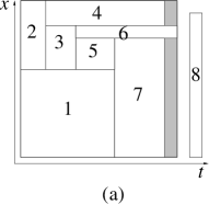
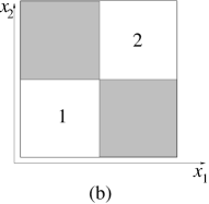
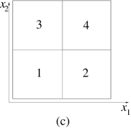
Figure 2: Differences between RCPSP and packing: (a) A set of jobs that is feasible for scheduling with one resource constraint, but infeasible for two-dimensional packing: Job 8 does not violate a resource constraint, but does not fit as a contiguous rectangle. (b) A set of jobs that is just feasible for RCPSP with $d=2$ constraints, i.e., that does not allow any tighten of either constraint without becoming infeasible. (c) A set of boxes that is just feasible for packing in $d=2$ dimensions.

Higher-dimensional packing problems (without order constraints) have been considered by a great number of authors, but only few of them have dealt with the exact solution of general two-dimensional problems. See [8, 10] for an overview. It should be stressed that unlike one-dimensional packing problems, higher-dimensional packing problems allow no straightforward formulation as integer programs: After placing one box in a container, the remaining feasible space will in general not be convex. Moreover, checking whether a given set of boxes fits into a particular container (the so-called orthogonal packing problem, OPP) is trivial in one-dimensional space, but NP-hard in higher dimensions.

Nevertheless, attempts have been made to use standard approaches of mathematical programming. Beasley [2] and Hadjiconstantinou and Christofides [17] have used a discretization of the available positions to an underlying grid to get a 0-1 program with a pseudopolynomial number of variables and constraints. Not surprisingly, this approach becomes impractical beyond instances of rather moderate size. More recently, Padberg [28] gave a mixed integer programming formulation for three-dimensional packing problems, similar to the one anticipated by Schepers [29] in his thesis. Padberg expressed the hope that using a number of techniques from branch-and-cut will be useful; however, he did not provide any practical results to support this hope.

In [7, 8, 10, 11, 31], a different approach to characterizing feasible packings and constructing optimal solutions is described. A graph-theoretic characterization of the relative position of the boxes in a feasible packing (by so-called packing classes) is used, representing $d$-dimensional packings by a $d$-tuple of interval graphs (called component graphs) that satisfy two extra conditions. This factors out a great deal of symmetries between different feasible packings, it allows to make use of a number of elegant graph-theoretic tools, and it reduces the geometric problem to a purely combinatorial one without using brute-force methods like introducing an underlying coordinate grid. Combined with good heuristics for dismissing infeasible sets of boxes [9], a tree search for constructing feasible packings was developed. This exact algorithm has been implemented; it outperforms previous methods by a clear margin.

For the benefit of the reader, a concise description of this approach is contained in Section 3.

Graph Theory of Order Constraints

In the context of scheduling with precedence constraints, a natural problem is the following, called transitive ordering with precedence constraints (TOP): Consider a partial order $P=(V,\prec)$ of precedence constraints and a (temporal) comparability graph $G=(V,E)$, such that all relations in $P$ are represented by edges in $G$. Is there a transitive orientation $D=(V,A)$ of $G$, such that $P$ is contained in $D$?

Korte and Möhring [20] have given a linear-time algorithm for deciding TOP, using modified PQ-trees. However, their approach requires knowledge of the full set of edges in $G$. When running a branch-and-bound algorithm for solving a scheduling problem, these edges of $G$ are only known partially during most of the tree search, but already this partial edge-set may prohibit the existence of a feasible solution for a given partial order $P$. This makes it desirable to come up with structural characterizations that are already useful when only parts of $G$ are known.

Such a set of precedence constraints may be described by a dependency graph, see Figure 3.

For a problem instance of this type, we describe a general framework for finding exact solutions to the problem of minimizing the height of a container of given base area, or minimizing the makespan of a higher-dimensional non-preemptive scheduling problem.

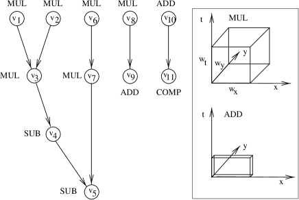
Figure 3: Dependency graph of jobs and shape of modules (3D boxes) with the spatial dimensions $x$ and $y$ and the temporal dimension $t$ (execution time).

Results of this paper

In this paper, we give the first exact study of higher-dimensional packing with order constraints, which can also be interpreted as higher-dimensional non-preemptive scheduling problems. We develop a general framework for problems of this type by giving a pair of necessary and sufficient conditions for the existence of a solution for the problem TOP on graphs $G$ in terms of forbidden substructures. Using the concept of packing classes, our conditions can be used quite effectively in the context of a branch-and-bound framework, because it can recognize infeasible subtrees at “high” branches of the search tree. In particular, we describe how to find an exact solution to the problem of minimizing the height of a container of given base area. If this third dimension represents time, this amounts to minimizing the makespan of a higher-dimensional scheduling problem. We validate the usefulness of these concepts and results by providing computational results. Other problem versions (like higher-dimensional knapsack or bin packing problems with order constraints) can be treated similarly.

The rest of this paper is organized as follows. In Section 2, we describe basic assumptions and some terminology. The notion of packing classes and a solution to packing problems without precedence constraints is summarized in Section 3. In Section 4, we introduce precedence constraints, describe the mathematical foundations for incorporating them into the search, and explain how to implement the resulting algorithms. Section 5 provides the necessary mathematical foundations for the correctness of our approach. Finally, we present computational results for a number of different benchmarks in Section 6.

2 Preliminaries

An FPGA consists of a rectangular grid of identical logic cells. Each job $v$ (or “module”) requires a rectangle of size $w_{x}(v)$ by $w_{y}(v)$ with fixed axis-parallel orientation, and needs to remain available for at least the time $w_{t}(v)$. Any logic cell that is not occupied by a module may be used by one of the rectangular jobs. As shown in Figure 1, we are dealing with a three-dimensional packing problem, possibly with order constraints. In the following, we describe technical as well as mathematical terminology and assumptions.

2.1 Architecture Assumptions

The model of having relocatable, rectangular modules is justified by current FPGA technology [1, 33].

Intermodule communication

Intermodule communication is assumed to occur at the end of operation of the sending module (task model). The issuing module may store its result register values into an external memory connected to the FPGA interface (read-out) via a bus interface. Memory is allocated for temporary storage of intermediate results. Afterwards, the receiving module will read the communicated data into its registers via the bus interface. With this communication style, it is justifiable to ignore routing overhead between modules that otherwise might introduce additional placement constraints.

I/O-overhead

The communication time needed for writing out and reading in communicated data may be accounted for by considering this as an offset and being part of the execution time of a job.

Reconfiguration overhead

The time needed for carrying out reconfigurations may be modeled by a constant (possibly a different number for each job), depending on the target architecture. This may be considered a simplification because the reconfiguration time might depend on the result of the placement. Consider two equal modules with identical placements. A reconfiguration for the second module might not be necessary in case no third module is occupying a (sub)set of cells in the time interval between the execution of the two modules. However, there are many different models for accounting for reconfiguration times, and the particular choice should be adapted individually to the target architecture.

2.2 Mathematical Terminology

Problem instances

We assume that a problem instance is given by a set $V$ of jobs. Each job has a spatial requirement in the $x$- and $y$-direction, denoted by $w_{x}(v)$ and $w_{y}(v)$, and a duration, denoted by a size $w_{t}(v)$ along the time axis. The available space $H$ consists of an area of size $h_{x}\times h_{y}$. In addition, there may be an overall allowable time $h_{t}$ for all jobs to be completed. A schedule is given by a start time $p_{t}(v)$ for each job. A schedule is feasible, if all jobs can be carried without preemption or overlap of computation jobs in time and space, such that all jobs are within spatial and temporal bounds.

Graphs

Some of our descriptions make use of a number of certain graph-theoretic concepts. An (undirected) graph $G=(V,E)$ is given by a set of vertices $V$, and a set of edges $E$; each edge describes the adjacency of a pair of vertices, and we write $\{u,w\}$ for an edge between vertices $u$ and $w$. We only consider graphs without multiple edges and without loops. For a graph $G$, we obtain the complement graph $\overline{G}$ by exchanging the set $E$ of edges with the set $\overline{E}$ of non-edges. In a directed graph $D=(V,A)$, edges are oriented, and we write $(u,w)$ to denote an edge directed from $u$ to $w$. A graph $G=(V,E)$ is a comparability graph if there is a transitive orientation for it, i.e., the edges $E$ can be oriented to a set of directed arcs $A$, such that we get the transitive closure of a partial order. More precisely, this means that $D=(V,A)$ is a cycle-free digraph for which the existence of edges $(u,v)\in A$ and $(v,w)\in A$ for any $u,v,w\in V$ implies the existence of $(u,w)\in A$. Comparability graphs have a variety of nice properties. For our purpose we will make use of the algorithmic result that computing maximum weighted cliques on comparability graphs can be done efficiently (see [16]). A closely related family of graphs, the interval graphs, are defined as follows. Given a set of intervals on the real line, every vertex of the graph corresponds to an interval of the set; two vertices are joined by an edge if the corresponding intervals have a non-empty intersection. Interval graphs have been studied intensively in graph theory (see [16, 25]), and, similar to comparability graphs, they have a number of very useful algorithmic properties.

Precedence constraints

Mathematically, a set of precedence constraints is given by a partial order $P=(V,\prec)$ on $V$. The relations in $\prec$ can be interpreted as a directed acyclic graph $D_{P}=(V,A_{P})$, where $A_{P}$ is a set of directed arcs corresponding to the relations in $\prec$. In the presence of such a partial order, a feasible schedule is required to satisfy the capacity constraints of the container, as well as these additional constraints.

Packing problems

In the following, we treat jobs as axis-aligned $d$-dimensional boxes with given orientation, and feasible schedules as arrangements of boxes that satisfy all side constraints. This is implied by the term of a feasible packing. There may be different types of objective functions, corresponding to different types of packing problems. The Orthogonal Packing Problem (OPP) is to decide whether a given set of boxes can be placed within a given “container” of size $h_{x}\times h_{y}\times h_{t}$. For the Constrained OPP (COPP), we also have to satisfy a partial order $P=(V,\prec)$ of precedence constraints in the $t$-dimension. To emphasize the motivation of temporal precedence constraints, we write $t$ to suggest that the time coordinate is constrained, and $x$ and $y$ to imply that the space coordinates are unrestricted. Although our application mainly requires to consider those temporal constraints, it should be mentioned that our approach works the same way when dealing with spatial restrictions; that is why we are using a generic index $i$ in the mathematical discussion, while some of our benchmark examples consider a temporal dimension $t$.

There are various optimization problems that have OPP or COPP as their underlying decision problems. The Base Minimization Problem (BMP) is to minimize the size $h_{x}$ for a fixed $h_{t}$ such that all boxes fit into a container $h_{x}\times h_{x}\times h_{t}$ with quadratic base. This corresponds to minimizing the necessary area to carry out a set of computations within a given time. Because our main motivation arises from dynamic chip reconfigurations, where we want to minimize the overall running time, we focus on the Constrained Strip Packing Problem (CSPP), which is to minimize the size $h_{t}$ for a given base size $h_{x}\times h_{y}$, such that all boxes fit into the container $h_{x}\times h_{y}\times h_{t}$. Clearly, we can use a similar approach for other objective functions.

3 Solving Unconstrained Orthogonal Packing Problems

3.1 A General Framework

If we have an efficient method for solving OPPs, we can also solve BMPs and SPPs by using a binary search. However, deciding the existence of a feasible packing is a hard problem in higher dimensions, and methods proposed by other authors [2, 17] have been of limited success.

Our framework uses a combination of different approaches to overcome these problems:

1. Try to disprove the existence of a packing by classes of lower bounds on the necessary size.

2. In case of failure, try to find a feasible packing by using fast heuristics.

3. If the existence of a packing is still unsettled, start an enumeration scheme in form of a branch-and-bound tree search.

By developing good new bounds for the first stage, we have been able to achieve a considerable reduction of the number of cases in which a tree search needs to be performed. (Mathematical details for this step are described in [9, 11].) However, it is clear that the efficiency of the third stage is crucial for the overall running time when considering difficult problems. Using a purely geometric enumeration scheme for this step by trying to build a partial arrangement of boxes is easily seen to be immensely time-consuming. In the following, we describe a purely combinatorial characterization of feasible packings that allows to perform this step more efficiently.

3.2 Packing Classes

Consider a feasible packing in $d$-dimensional space, and project the boxes onto the $d$ coordinate axes. This converts the one $d$-dimensional arrangement into $d$ one-dimensional ones (see Figure 4 for an example in $d=2$). By disregarding the exact coordinates of the resulting intervals in direction $i$ and only considering their intersection properties, we get the component graph $G_{i}=(V,E_{i})$: Two boxes $u$ and $v$ are connected by an edge in $G_{i}$, iff their projected intervals in direction $x_{i}$ have a non-empty intersection. By definition, these graphs are interval graphs.

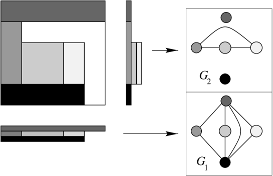
Figure 4: The projections of the boxes onto the coordinate axes define interval graphs (here in 2D: $G_{1}$ and $G_{2}$).

Considering sets of $d$ component graphs $G_{i}$ instead of complicated geometric arrangements has some clear advantages (algorithmic implications for our specific purposes are discussed further down). It is not hard to check that the following three conditions must be satisfied by all $d$-tuples of graphs $G_{i}$ that are constructed from a feasible packing:

1. $G_{i}$ is an interval graph, $\forall i\in\{1,\cdots,d\}$.

2. Any independent set $S$ of $G_{i}$ is $i$-admissible, $\forall i\in\{1,\cdots,d\}$, i.e., $w_{i}(S)=\sum_{v\in S}w_{i}(v)\leq h_{i}$, because all boxes in $S$ must fit into the container in the $i$th dimension.

3. $\cap_{i=1}^{d}E_{i}=\emptyset$. In other words, there must be at least one dimension in which the corresponding boxes do not overlap.

A $d$-tuple of component graphs satisfying these necessary conditions is called a packing class. The remarkable property (proven in [29, 10]) is that these three conditions are also sufficient for the existence of a feasible packing.

Theorem 1 (Fekete, Schepers).

A set of $d$-dimensional boxes allows a feasible packing, iff there is a packing class, i.e., a $d$-tuple of graphs $G_{i}=(V,E_{i})$ that satisfies the conditions C1, C2, C3.

This allows us to consider only packing classes in order to decide the existence of a feasible packing, and to disregard most of the geometric information.

3.3 Solving OPPs

Our search procedure works on packing classes, i.e., $d$-tuples of component graphs with the properties C1, C2, C3. Because each packing class represents not only a single packing but a whole family of equivalent packings, we are effectively dealing with more than one possible candidate for an optimal packing at a time. (The reader may check for the example in Figure 4 that there are 36 different feasible packings that correspond to the same packing class.)

For finding an optimal packing, we use a branch-and-bound approach. The search tree is traversed by depth first search, see [7, 29] for details. Branching is done by deciding about a single pair of vertices $b,c$, whether the corresponding edge is contained in $E_{i}$ or is not contained in $E_{i}$, i.e., $\{b,c\}\in E_{i}$ or $\{b,c\}\notin E_{i}$. So in fact, there are three classes of edges; those which are fixed to be in $E_{i}$, those which are fixed not to be in $E_{i}$ (non-edges), and those for which it is not decided yet whether they will be contained in $E_{i}$ or not. After each branching step, it is checked whether one of the three conditions C1, C2, C3 is violated with respect to the currently fixed edges and non-edges; furthermore it is checked whether a violation can only be avoided by fixing further (formerly undecided) edges or non-edges. Testing for two of the conditions C1–C3 is easy: enforcing C3 is obvious; checking C2 can be done efficiently, since $\overline{G}_{i}$ is a comparability graph and, as mentioned before, in those graphs maximum weighted cliques can be done efficiently. Note that for this step only non-edges are used, i.e., pairs of vertices for which has been decided already that they are not contained in $E_{i}$. In order to ensure that property C1 is not violated, we use some graph-theoretic characterizations of interval graphs and comparability graphs. These characterizations are based on two forbidden substructures. (Again, see [16] for details; the first condition is based on the classical characterizations by [14, 15]: a graph is an interval graph iff its complement has a transitive orientation, and it does not contain any induced chordless cycle of length 4.) In particular, the following configurations have to be avoided:

1. induced chordless cycles of length 4 in $E_{i}$;

2. so-called 2-chordless odd cycles in the set of edges excluded from $E_{i}$ (see [7, 16] for details);

3. infeasible stable sets in $E_{i}$.

Each time we detect such a fixed subgraph, we can abandon the search on this node. Furthermore, if we detect a fixed subgraph, except for one unfixed edge, we can fix this edge, such that the forbidden subgraph is avoided.

Our experience shows that in the considered examples these conditions are already useful when only small subsets of edges have been fixed, because by excluding small sub-configurations like induced chordless cycles of length 4, each branching step triggers a cascade of more fixed edges.

4 Packing Problems with Precedence Constraints

As mentioned in the above discussion, a key advantage of considering packing classes is that it makes possible the consideration of packing problems independent of precise geometric placement, and that it allows arbitrary feasible interchanges of placements. However, for most practical instances, we have to satisfy additional constraints for the temporal placement, i.e., for the relative start times of jobs. For our approach, the nature of the data structures may simplify these problems from three-dimensional to purely two-dimensional ones: If the whole schedule is given, all edges $E_{t}$ in one of the graphs are determined, so we only need to construct the edge sets $E_{x}$ and $E_{y}$ of the other graphs. As worked out in detail in [30, 31], this allows it to solve the resulting problems quite efficiently if the arrangement in time is already given.

A more realistic, but also more involved situation arises if only a set of precedence constraints is given, but not the full schedule. We describe in the following how further mathematical tools in addition to packing classes allow useful algorithms. Note that our method of dealing with order constraints is not restricted to one (the temporal) dimension; in fact, we can also deal with constraints in several dimensions at once, as demonstrated in Section 6, Figure 14.

4.1 Packing Classes and Interval Orders

Any edge $\{v_{1},v_{2}\}$ in a component graph $G_{i}$ corresponds to an intersection between the projections of boxes $1$ and $2$ onto the $x_{i}$-axis. This means that the complement graph $\overline{G_{i}}$ given by the complement $\overline{E_{i}}$ of the edge set $E_{i}$ consists of all pairs of coordinate intervals that are “comparable”: Either the first interval is “to the left” of the second, or vice versa.

Any (undirected) graph of this type is a comparability graph. By orienting edges to point from “left” to “right” intervals, we get a partial order of the set $V$ of vertices, a so-called interval order [12, 25]. Obviously, this order relation is transitive, inducing a transitive orientation on the (undirected) comparability graph $G_{i}$. See Figure 5 for a (two-dimensional) example of a packing class, the corresponding comparability graphs, the transitive orientations, and the packing corresponding to the transitive orientations.

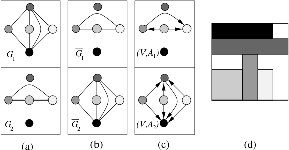
Figure 5: (a) A two-dimensional packing class. (b) The corresponding comparability graphs. (c) Two transitive orientations. (d) A feasible packing corresponding to the orientation.

Now consider a situation where we need to satisfy a partial order $P=(V,A_{P})$ of precedence constraints in the time dimension. It follows that each arc $a=(u,w)\in A_{P}$ in this partial order forces the corresponding undirected edge $e=\{u,w\}$ to be excluded from $E_{i}$. Thus, we can simply initialize our algorithm for constructing packing classes by fixing all undirected edges corresponding to $A_{P}$ to be contained in $\overline{E_{i}}$. After running the original algorithm, we may get additional comparability edges. As the example in Figure 6 shows, this causes an additional problem: Even if we know that the graph $\overline{G_{i}}$ has a transitive orientation, and all arcs $a=(u,w)$ of the precedence order $(V,A_{P})$ are contained in $\overline{E_{i}}$ as $e=\{u,w\}$, it is not clear that there is a transitive orientation that contains all arcs of $A_{P}$.

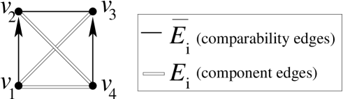
Figure 6: A comparability graph $\overline{G_{i}}=(V,\overline{E_{i}})$ with a partial order $P$ contained in $\overline{E_{i}}$, such that there is no transitive orientation of $\overline{G_{i}}$ that extends $P$.

4.2 Extending Partial Suborders

Consider a comparability graph $\overline{G}$ that is the complement of an interval graph $G$. The problem TOP of deciding whether $\overline{G}$ has a transitive orientation that extends a given partial order $P$ has been studied in the context of scheduling. Korte and Möhring [20] give a linear-time algorithm for determining a solution, or deciding that none exists. Their approach is based on a very special data structure called modified PQ-trees.

In principle it is possible to solve higher-dimensional packing problems with precedence constraints by adding this algorithm as a black box to test the leaves of our search tree for packing classes: In case of failure, backtrack in the tree. However, the resulting method cannot be expected to be reasonably efficient: During the course of our tree search, we are not dealing with one fixed comparability graph, but only build it while exploring the search tree. This means that we have to expect spending a considerable amount of time testing similar leaves in the search tree, i.e., comparability graphs that share most of their graph structure. It may be that already a very small part of this structure that is fixed very “high” in the search tree constitutes an obstruction that prevents a feasible orientation of all graphs constructed below it. So a “deep” search may take a long time to get rid of this obstruction. This makes it desirable to use more structural properties of comparability graphs and their orientations to make use of obstructions already “high” in the search tree.

4.3 Implied Orientations

As in the basic packing class approach, we consider the component graphs $G_{i}$ and their complements, the comparability graphs $\overline{G_{i}}$. This means that we continue to have three basic states for any edge:

1. edges that have been fixed to be in $E_{i}$, i.e., component edges;

2. edges that have been fixed to be in $\overline{E_{i}}$, i.e., comparability edges;

3. unassigned edges.

In order to deal with precedence constraints, we also consider orientations of the comparability edges. This means that during the course of our tree search, we can have three different possible states for each comparability edge:

1. one possible orientation;

2. the opposite possible orientation;

3. no assigned orientation.

A stepping stone for this approach arises from considering the following two configurations; see Figure 7.

\psfrag{(I)}{(I)}\psfrag{(II)}{(II)}\psfrag{(III)}{(III)}\psfrag{(I')}{(I')}\psfrag{(II')}{(II')}\psfrag{(III')}{(III')}\psfrag{(D1)}{(D1)}\psfrag{(D2)}{(D2)}\psfrag{v-1}{$v_{1}$}\psfrag{v-2}{$v_{2}$}\psfrag{v-3}{$v_{3}$}\psfrag{Eb}{$\overline{E}$}\psfrag{E}{$E$}\psfrag{(comparability edges)}{{\scriptsize(comparability edges)}}\psfrag{(component edges)}{{\scriptsize(component edges)}}\psfrag{unassigned or}{{\scriptsize(unassigned or}}\psfrag{comparability edges}{{\scriptsize comparability edges)}}\includegraphics[width=369.88582pt]{all-new}

Figure 7: Implications for edges and their orientations: Above are $P_{3}$ implications (D1, left) and transitivity implications (D2, right); below the forced orientations of edges.

The first configuration (shown in the left part of the figure) consists of the two comparability edges $\{v_{1},v_{2}\}$, $\{v_{2},v_{3}\}$ $\in\overline{E_{i}}$, such that the third edge $\{v_{1},v_{3}\}$ has been fixed to be an edge in the component graph $E_{i}$. Now any orientation of just one of the comparability edges forces the orientation of the other comparability edge. In Figure 7 the oriented edge in (I) forces the orientation of the second edge as shown in (I’), similarly for (II) and (II’). Because this configuration corresponds to an partially oriented induced path on three vertices, a $P_{3}$ in $\overline{G_{i}}$, we call this arrangement a $P_{3}$ implication.

The second configuration (shown in the right part of the figure) consists of two directed comparability edges $(v_{1},v_{2}),(v_{2},v_{3})$. In this case we know that edge $\{v_{1},v_{3}\}$ must also be a comparability edge, with an orientation of $(v_{1},v_{3})$. Because this configuration arises directly from transitivity in $\overline{G_{i}}$, we call this arrangement a transitivity implication.

Clearly, any implication arising from one of the above configurations can induce further implications.

In particular, when considering only sequences of $P_{3}$ implications, we get a partition of comparability edges into $P_{3}$ implication classes that will be used in more detail in Section 5. Two comparability edges are in the same $P_{3}$ implication class, iff there is a sequence of $P_{3}$ implications, such that orienting one edge forces the orientation of the other edge. It is not hard to see that the $P_{3}$ implication classes form a partition of the comparability edges, because we are dealing with an equivalence relation. For an example, consider the arrangement in Figure 6. Here, all three comparability edges $\{v_{1},v_{2}\}$, $\{v_{2},v_{3}\}$, and $\{v_{3},v_{4}\}$ are in the same $P_{3}$ implication class. Now the orientation of $(v_{1},v_{2})$ implies the orientation $(v_{3},v_{2})$, which in turn implies the orientation $(v_{3},v_{4})$, contradicting the orientation of $\{v_{3},v_{4}\}$ in the given partial order $P$.

We call a violation of a $P_{3}$ implication a $P_{3}$ conflict.

As the example in Figure 8 shows, only excluding $P_{3}$ conflicts when recursively carrying out $P_{3}$ implications does not suffice to guarantee the existence of a feasible orientation: Working through the queue of $P_{3}$ implications, we end up with a directed cycle, which violates a transitivity implication.

Figure 8: (a) A graph $\overline{G_{i}}$ with a partial order formed by three directed edges; (b) there are three $P_{3}$ implication classes that each have one directed arc; (c) carrying out $P_{3}$ implications creates directed cycles, i.e., transitivity conflicts.

We call a violation of a transitivity implication a transitivity conflict.

Summarizing, we have the following necessary conditions for the existence of a transitive orientation that extends a given partial order $P$:

1. Any $P_{3}$ implication can be carried out without a conflict.

2. Any transitivity implication can be carried out without a conflict.

These necessary conditions are also sufficient:

Theorem 2.

Let $P=(V,<)$ be a partial order with arc set $A_{P}$ that is contained in the edge set $E$ of a given comparability graph $G=(V,E)$. $A_{P}$ can be extended to a transitive orientation of $G$, iff all arising $P_{3}$ implications and transitivity implications can be carried out without creating a $P_{3}$ conflict or a transitivity conflict.

A full proof and further mathematical details are described in the following Section 5. This extends previous work by Gallai [13], who extensively studied implication classes of comparability graphs. See Kelly [19], Möhring [25] for helpful surveys on this topic, and Krämer [22] for an application in scheduling theory.

5 Extending Partial Orientations

Modular decomposition

The concept of modular decomposition of a graph was first introduced by Gallai [13] for studying comparability graphs. This powerful decomposition scheme has a variety of applications in algorithmic graph theory; for further material on this concept and its application the interested reader is referred to [19, 26].

A module of a graph $G=(V,E)$ is a vertex set $M\subseteq V$ such that each vertex $v\in V\setminus M$ is either adjacent to all vertices or to no vertex of $M$ in $G$. (Intuitively speaking, all vertices of a module “look the same” to the other vertices of the graph.) A module is called trivial if $|M|\leq 1$ or $M=V$. A graph $G$ is called prime if it contains only trivial modules. Using the concept of modules one can define a decomposition scheme for general graphs by decomposing it recursively into subsets, each of which is a module of $G$, stopping when all sets are singletons. First of all, observe that every connected component of a given graph $G$ forms a module. It is not hard to see that also every co-connected component of $G$ is a module. If both $G$ and its complement are connected then the decomposition needs a further idea. Consider the graph in Figure 9. Obviously it is connected and co-connected and has a huge number of non-trivial modules. However, if one identifies the maximal proper submodules of $G$, i.e., those modules $M$ that are inclusion-maximal modules of $G$ with $M\not=V$, then one obtains a partition of the vertex set. The corresponding modules of the example $G$ are $M_{1}=\{0$, $1$, $2$, $3$, $4$, $5$, $6$, $7$, $8$, $9\}$, $M_{2}=\{20\}$, $M_{3}=\{10,11\}$, $M_{4}=\{12,13,14,15,16,17,18$, $19\}$.

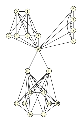
Figure 9: An example graph $G$.

Gallai [13] showed that any graph $G$ has a particular decomposition (the so-called canonical decomposition) of its vertex set into a set of modules with a variety of nice properties. He observed that any graph $G$ is either of parallel type, i.e., $G$ is not connected; or $G$ is of series type, i.e., $\overline{G}$ is not connected, or $G$ is of prime type, i.e., $G$ and $\overline{G}$ are connected. In the first case the canonical decomposition is defined by the set of connected components; in the second case the canonical decomposition is given by the connected components of $\overline{G}$; finally, for prime-type graphs, the canonical decomposition is given by decomposing $G$ into its maximal proper submodules. Gallai also showed that this decomposition is unique.

This recursive decomposition defines a decomposition tree $T(G)$ for a given graph $G$ in a very natural way: Create a root vertex of $T(G)$ for the trivial module $G$ itself. Label it series, parallel, or prime, depending on the type of $G$. For each non-singleton module of the canonical decomposition of $G$ create a tree vertex, labeled as series-, parallel-, or prime-type node, depending on the type of the module, and make it a child of the vertex corresponding to $G$; for each singleton module add a tree-vertex labeled with the corresponding singleton. Now proceed recursively for each subgraph corresponding to a non-trivial module in the decomposition tree, until all leaves of the tree are labeled with singletons. Consequently, the leaves of the tree correspond to the vertices of the graph, while all internal vertices correspond to non-trivial modules of the canonical decomposition of the corresponding parent vertex in $T(G)$. See Figure 10 for the decomposition tree of our example.

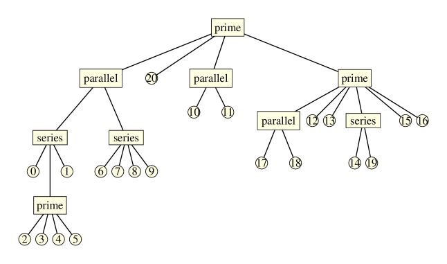
Figure 10: A modular decomposition tree for the graph $G$ shown in Figure 9.

The decomposition graph $G^{\#}$ of a graph $G$ is the quotient of $G$ by the canonical decomposition into the set of modules $\{A_{1},\dots,A_{q}\}$, i.e., $V(G^{\#})=\{A_{1},\dots,A_{q}\}$, and distinct vertices $A_{i}$ and $A_{j}$ are joined by an edge in $G^{\#}$ iff there is an $A_{i}A_{j}$-edge in $G$. In the following we will look at the decomposition graphs corresponding to internal vertices of $T(G)$ and refer to them as the decomposition graphs of $T$.

In our example, the decomposition graph $G^{\#}$ of $G$, i.e., to the root node of $T(G)$, is a path on four vertices, given by

$$G^{\#}=(\{M_{1},M_{2},M_{3},M_{4}\},\{\{M_{1},M_{2}\},\{M_{2},M_{3}\},\{M_{3},M_{4}\}\}).$$

Modular decomposition and transitive orientations

An important property of the modular decomposition is its close relationship to the concept of $P_{3}$ implication classes. Gallai observed the following properties of $P_{3}$ implication classes with respect to the modular decomposition:

Proposition 3 (Gallai [13]).

Let $G=(V,E)$ be an undirected graph.

1. If $G$ is not connected and $G_{1},\dots,G_{q}$ ($q\geq 2$) are the components of $G$, then the $P_{3}$ implication classes of $G_{1},\dots,G_{q}$ are exactly the $P_{3}$ implication classes of $G$.

2. If $\overline{G}$ is not connected (so that $G$ is connected), $\overline{G_{1}},\dots,\overline{G_{q}}$ ($q\geq 2$) are the components of $\overline{G}$, and $A_{i}=V(G_{i})$, then $A_{i}$ and $A_{j}$ are completely connected to each other whenever $1\leq i<j\leq q$. Moreover, for all such $i$ and $j$, the set of $A_{i}A_{j}$-edges form an $P_{3}$ implication class $E_{ij}$ of $G$. The $P_{3}$ implication classes of $G$ that are distinct from any $E_{ij}$ are exactly the $P_{3}$ implication classes of the graphs $G_{i}=G[A_{i}]$ ($i=1,\dots,q$).

3. If $G$ and $\overline{G}$ are both connected and have more than one vertex, and the canonical decomposition of $G$ is given by $\{A_{1},\dots,A_{q}\}$, then we have

   1. If there is one edge between $A_{i}$ and $A_{j}$ ($1\leq i<j\leq q$), then all edges between $A_{i}$ and $A_{j}$ are in $G$.

   2. The set of all edges of $G$ that join different $A_{i}$s forms a single $P_{3}$ implication class $C$ of $G$. Every vertex of $G$ is incident with some edge of $C$, (i.e., $V(C)=V(G)$).

   3. The $P_{3}$ implication classes of $G$ that are distinct from $C$ are exactly the $P_{3}$ implication classes of the graphs $G_{i}=G[A_{i}]$ ($1\leq i\leq q$).

This strong relationship between $P_{3}$ implication classes and the modules in the canonical decomposition of a given graph is a powerful tool for studying graphs having a transitive orientation. Note that the fastest known algorithms for recognizing comparability graphs make extensively use of this relationship. Gallai used the above properties (among others) for proving the following theorem.

Theorem 4 (Gallai [13]).

Let $G$ be a non-empty graph, let $T=T(G)$ be the tree decomposition of $G$, and let $H$ be a vertex set corresponding to a node of $T$.

1. If $G$ is transitively oriented, and $A$ and $B$ are descendents of $H$ in $T$, then every $A,B$-edge of $G$ is oriented in the same direction (to or from $A$). Therefore, $H^{\#}$ receives an induced transitive orientation.

2. Conversely, assuming that $H^{\#}$ is transitively orientable for each $H\in T$, one can choose an arbitrary transitive orientation of each $H^{\#}$ and induce a transitive orientation of $G$ by orienting all $A,B$-edges (for $A$ and $B$ descendents of $H$ in $T$) in the same direction that $\{A,B\}$ is oriented in $H^{\#}$.

It is straightforward to draw the following helpful corollaries from this theorem:

Corollary 5.

A graph $G$ is a comparability graph if and only if every decomposition graph in the tree decomposition of $G$ is a comparability graph.

Corollary 6.

Let $G$ be a comparability graph and $T$ its tree decomposition. Assigning to each of the decomposition graphs of $T$ a transitive orientation independently results in a transitive orientation of $G$.

Furthermore, if only a partial orientation of $G$ is given and we are interested in extending this orientation to a transitive orientation of $G$, we can formulate the following lemma.

Lemma 7.

Let $G$ be a comparability graph and $T$ its tree decomposition. Furthermore, let $P$ be a partial orientation of $G$, assigning orientations to some, but not all $P_{3}$ implication classes of $G$. $P$ is extendible to a transitive orientation of $G$ if and only if for each decomposition graph $H^{\#}$ of $T$ the orientation induced on $H^{\#}$ by $P$ is extendible to a transitive orientation on $H^{\#}$.

Proof: Follows immediately from Theorem 4 (2). $\Box$

Now we are ready to prove Theorem 2: Conditions D1 and D2 are also sufficient.

Proof of Theorem 2:

Suppose there is a transitive orientation $F$ of $G$ that contains $P$. Because $F$ is a transitive orientation, all arcs implied by $P_{3}$ or transitivity implications are contained in $F$. Furthermore, there cannot be any $P_{3}$ or transitivity conflict in $F$, again because $F$ is a transitive orientation. Thus $F$ shows that all arising $P_{3}$ and transitivity implications can be carried out without creating a $P_{3}$ or transitivity conflict.

Suppose now that D1 and D2 are satisfied, i.e., there is a directed graph $F$ consisting of all arcs of $P$ together with all orientations of edges of $G$ that are implied by a sequence of $P_{3}$ and transitivity implications of arcs of $P$. In other words, $F$ contains all arcs that are forced by $P_{3}$ or transitivity implications together with all their implied arcs; i.e., all arcs that are forced by arcs of $F$ are also contained in $F$. We show that $F$ can be extended to a transitive orientation of $G$.

First observe that, by assumption, there cannot be a $P_{3}$ or transitivity conflict in $F$. In particular, $F$ is an orientation of edges of $G$ and for each $P_{3}$ implication class $C$ of $G$ that has at least one edge that is oriented in $F$, all edges of $C$ are oriented in $F$ and this orientation is conflict-free. By Corollary 6, every single conflict-free oriented $P_{3}$ implication class of $G$ by itself is extendible to a transitive orientation of $G$.

Now let $T$ be the decomposition tree of $G$ and consider the decomposition graphs corresponding to $T$. By the above observation, the orientation of an $P_{3}$ implication class $C$ in $F$ implies an orientation of the edge(s) corresponding to this $P_{3}$ implication class in the decomposition graphs of $T$. More precisely, by Observation 3 (2), for every series-type node $H$ of $T$ each edge $e=\{AB\}$ of $H^{\#}$ corresponds exactly to one $P_{3}$ implication class $C_{e}$ of $G$. If $C_{e}$ is oriented conflict-free in $F$, this orientation directly induces an orientation of $e$ (see Theorem 4). For a prime-type node $H$ the set of edges joining different $A_{i}$s forms exactly one $P_{3}$ implication class $C_{E}$ of $G$ (see Observation 3 (3)). Again, if $C_{E}$ is oriented conflict-free in $F$, this orientation immediately implies an orientation on $H^{\#}$.

All we have to show now is that for each decomposition graph $H^{\#}$ of $T$, the partial orientation implied by $F$ can be extended to a transitive orientation of $H^{\#}$. Then, by Corollary 6, the implied orientation of $G$ is transitive.

By Corollary 6, a parallel-type node of $T$ cannot create a contradiction to transitivity—it does not contain any edges.

Also a prime-type node of $T$ cannot create a contradiction: All of its edges are contained in only one $P_{3}$ implication class and, because all $P_{3}$ implication classes of $G$ contained in $F$ are oriented conflict-free, the corresponding orientation induced by $F$ on this single $P_{3}$ implication class has to be transitive.

This leaves the case of series-type nodes. Suppose there is a series-type node $H$ of $T$ with decomposition graph $H^{\#}$, for which the partial orientation implied by $F$ cannot be extended to a transitive orientation of $H^{\#}$. Then we claim that this partial orientation has to be cyclic: By definition for each series-type node $H$ of $T$ the decomposition graph $H^{\#}$ is a complete graph and every acyclic partial orientation of a complete graph can be extended to a transitive orientation of this complete graph by taking any topological ordering of the vertices that agrees with the partial orientation. Hence, the partial orientation on $H^{\#}$ has to contain a directed cycle.

However, by the definition of $T$ and the implied orientation of $H^{\#}$ by $F$, a directed cycle in $H^{\#}$ immediately implies a cyclically oriented cycle in $F$. Furthermore, with every consecutive pair of oriented edges $(x,y)$, $(y,z)$ of this cycle also the oriented edge $(x,z)$ (which is implied by transitivity) has to be contained in $F$. Iterating this argument results in an cyclically oriented triangle in $F$, which is a transitivity conflict. This contradicts our assumption that there are no transitivity conflicts. $\Box$

6 Computational Experiments

6.1 Solving Problems with Precedence Constraints

We start by fixing for all arcs $(u,v)\in A_{P}$ the edge $\{u,v\}$ as an edge in the comparability graph $\overline{G_{i}}$, and we also fix its orientation to be $(u,v)$. In addition to the tests for enforcing the conditions for unoriented packing classes (C1, C2, C3), we employ the implications suggested by conditions D1 and D2. For this purpose we check directed edges in $\overline{G_{i}}$ for being part of a triangle that gives rise to either implication. Any newly oriented edge in $\overline{G_{i}}$ gets added to a queue of unprocessed edges. Like for packing classes, we can again get cascades of fixed edge orientations. If we get an orientation conflict or a cycle conflict, we can abandon the search on this tree node. The correctness of the overall algorithm follows from Theorem 2; in particular, the theorem guarantees that we can carry out implications in an arbitrary order. In the following we present our results for different types of instances: The video-codec benchmark described in Section 6.3 arises from an actual application to FPGAs. In Section 6.4 we give a number of results arising from different geometric packing problems.

Our code was implemented in C++ and was run on a SUN Ultra 10 with 333 MHz.

The first example is a numerical method for solving a differential equation (DE) with 11 nodes. The node operations are either multiplications or ALU-type operations. In a second example, a video-codec using the H.261 norm is optimized. These examples are meant to demonstrate the general applicability of our method for practical problems; given other problem instances, or additional constraints, we can easily adapt our algorithm.

6.2 DE Benchmark

Let the module library contain two hardware modules (box types): an array-multiplier and a module of type ALU that realizes all other node operations (comparison, addition, subtraction). For a word-length of n=16 bits, we assume a module geometry of 16 x 1 cells for the ALU module, and of 16 x 16 cells for the multiplier. Furthermore, the execution time of an ALU node takes one clock cycle, while a multiplication requires 2 clock cycles on our target chip.

The dependency graph is shown in Fig. 3. First, we compute the transitive closure of all data dependencies to allow our algorithm to find contradictions to feasible packings already in the input.

Next, we solve several instances of the BMP problem for different values of $h_{t}$ reported in Table 1. Each $h_{t}$ listed yields a test case for which the container size is minimized (MinA ), assuming $h_{x}=h_{y}$. Also shown is the CPU-time needed for finding a solution.

Table 1: Computational results for optimizing reconfigurations for the DE benchmark.

test	container sizes
	$h_{t}$	$h_{x}$	$h_{y}$	CPU-time
1	6	32	32	55.76 s
2	13	17	17	0.04 s
3	14	16	16	0.03 s

The reported optimization times were measured as the CPU-times on a SUN-Ultra 10 with 333 MHz.

For the DE benchmark, it turns out that a chip of 32 x 32 freely programmable cells is necessary to obtain a latency between 6 and 12 clock cycles. As the longest path in the graph has length 6, there does not exist any faster schedule. For 12 and 13 cycles, a chip of size 17 x 17 is necessary, for $h_{t}\geq 14$, a chip of size 16 x 16 cells is sufficient, which is the smallest chip possible to implement the problem, as one multiplication by itself uses the full chip.

The SPP is solved in a similar way. The tradeoff between area size and necessary time is visualized in Fig. 11, in which the Pareto-optimal points are shown. The figure also shows the Pareto points for the case where no partial order needs to be satisfied (shown dashed).

Figure 11: Pareto-optimal points for minimizing chip area and processing time for the DE benchmark. (a) Including partial order constraints (solid lines). (b) Without consideration of partial order constraints (dashed lines).

6.3 Video-Codec Benchmark

Figure 12 shows a block diagram of the operation of a hybrid image sequence coder/decoder that arises from the FPGA application. The purpose of the coder is to compress video images using the H.261 standard. In this device, transformative and predictive coding techniques are unified. The compression factor can be increased by a predictive method for motion estimates: blocks inside a frame are predicted from blocks of previous images.

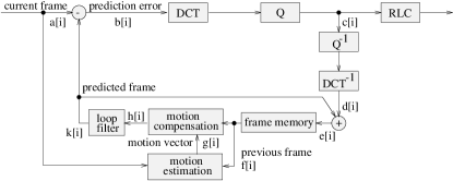
Figure 12: Block diagram of a video-codec (H.261).

The blocks of the operational description shown in the figure possess the granularity of more complex functions. However, this description contains no information corresponding to timing, architecture, and mapping of blocks onto an architecture. The resulting problem graph contains a subgraph for the coder and one subgraph for the decoder.

For realizing the device we have a library of three different modules. One is a simple processor core with a (normalized) area requirement of 625 units (25 x 25 cells, normalized to other modules in order to obtain a coarser grid) called PUM, denoted by “P” in Table 2. Secondly, there are two dedicated special-purpose modules: a block matching module (BMM), “B” in Table 2) that is used for motion estimation and requires 64 x 64 = 4096 cells; and a module DCTM (“D” in Table 2) for computing DCT/IDCT-computations, requiring 16 x 16 = 256 cells. Again, the BMP and the CSPP were considered, and the makespan was minimized for different latency constraints. Here there is only one Pareto-point found, shown in Table 2.

Table 2: Optimizing reconfigurations for the Video-Codec.

test	container sizes
	$h_{t}$	$h_{x}$	$h_{y}$	CPU-time
1	59	64	64	24.87 s

6.4 Geometric Instances

We describe computational results for two types of two-dimensional objects. See Table 3 for an overview. The first class of instances was constructed from a particularly difficult random instance of the 2-dimensional knapsack problem (see [8]). Results are given for order constraints of increasing size. In order to give a better idea of the computational difficulty, we give separate running times for finding an optimal feasible solution, and for proving that this solution is best possible.

Table 3: Optimal packing with order constraints.

instance	optimal		upper	lower
	$h_{t}$	$h_{x}$	bound	bound
okp17-0	169	100	7.29 s	179 s
okp17-1	172	100	6.73 s	1102 s
okp17-2	182	100	5.39 s	330 s
okp17-3	184	100	236 s	553 s
okp17-4	245	100	0.17 s	0.01 s
square21-no	112	112	84.28 s	0.01 s
square21-mat	117	112	15.12 s	277 s
square21-tri	125	112	107 s	571 s
square21-2mat	[118,120]	[118,120]	346 s	476 s

See Table 3 for the exact sizes of the 17 rectangles involved, and Figure 13 for the geometric layout of optimal packings. For easier reference, the boxes in the okp17 instances are labeled 1-17 in the given order.

The second class of instances arises from the well-known tiling of a 112x112 square by 21 squares of different sizes. Again we have added order constraints of various sizes. For the instance square21-2mat (with order constraints in two dimensions), we could not close the gap between upper and lower bound. For this instance we report the running times for achieving the best known bounds. Layouts of best solutions are shown in Figure 14.

Table 4: The problem instances okp17.

okp17:	base width of container = 100, number of boxes = 17
sizes =	[(8,81),(5,76),(42,19),(6,80),(41,48),(6,86),(58,20),(99,3),(9,52),
	(100,14),(7,53),(24,54),(23,77),(42,32),(17,30),(11,90),(26,65)]
okp17-0:	no order constraints
okp17-1:	11$\rightarrow$8, 11$\rightarrow$16
okp17-2:	11$\rightarrow$8, 11$\rightarrow$16, 8$\rightarrow$16
okp17-3:	11$\rightarrow$8, 11$\rightarrow$16, 8$\rightarrow$16, 8$\rightarrow$17, 11$\rightarrow$7, 16$\rightarrow$7
okp17-4:	11$\rightarrow$8, 11$\rightarrow$16, 8$\rightarrow$16, 8$\rightarrow$17, 11$\rightarrow$7, 16$\rightarrow$7, 17$\rightarrow$16

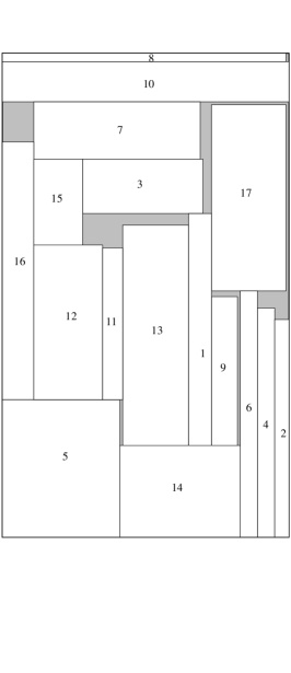
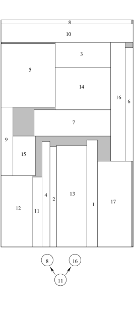
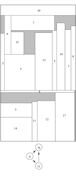
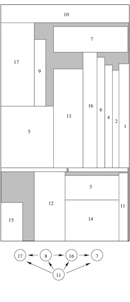
Figure 13: (a) An optimal packing of okp17-0 of height 169; (b) an optimal packing of okp17-1 of height 172; (c) an optimal packing of okp17-2 of height 182; (d) An optimal packing of okp17-3 of height 184.

Table 5: The problem instances square21.

square21:	base width of container = 112, number of boxes = 21
sizes =	[(50,50),(42,42),(37,37),(35,35),(33,33),(29,29),(27,27),(25,25),
	(24,24),(19,19),(18,18),(17,17),(16,16),(15,15),(11,11),(9,9),(8,8),
	(7,7),(6,6),(4,4),(2,2)]
square21-0:	no order constraints
square21-mat:	2$\rightarrow$4, 6$\rightarrow$7, 8$\rightarrow$9, 11$\rightarrow$15, 16$\rightarrow$17, 18$\rightarrow$19, 24$\rightarrow$25, 27$\rightarrow$29,
	33$\rightarrow$35, 37$\rightarrow$42, 2$\rightarrow$50, 50$\rightarrow$4
square21-tri:	2$\rightarrow$15, 15$\rightarrow$17, 2$\rightarrow$27, 4$\rightarrow$16, 16$\rightarrow$29, 4$\rightarrow$29, 6$\rightarrow$17, 17$\rightarrow$33,
	6$\rightarrow$33, 7$\rightarrow$18, 18$\rightarrow$35, 7$\rightarrow$35, 8$\rightarrow$19, 19$\rightarrow$37, 8$\rightarrow$37, 9$\rightarrow$24,
	24$\rightarrow$42, 9$\rightarrow$42, 11$\rightarrow$25, 25$\rightarrow$50, 11$\rightarrow$50
square21-2mat:	$x$-constraints:
	2$\rightarrow$19, 6$\rightarrow$25, 8$\rightarrow$29, 11$\rightarrow$35, 16$\rightarrow$42, 18$\rightarrow$4, 24$\rightarrow$7, 27$\rightarrow$9,
	33$\rightarrow$15, 37$\rightarrow$17, 50$\rightarrow$4, 18$\rightarrow$50
	$y$-constraints:
	2$\rightarrow$4, 6$\rightarrow$7, 8$\rightarrow$9, 11$\rightarrow$15, 16$\rightarrow$17, 18$\rightarrow$19, 24$\rightarrow$25, 27$\rightarrow$29,
	33$\rightarrow$35, 37$\rightarrow$42, 2$\rightarrow$50, 50$\rightarrow$4

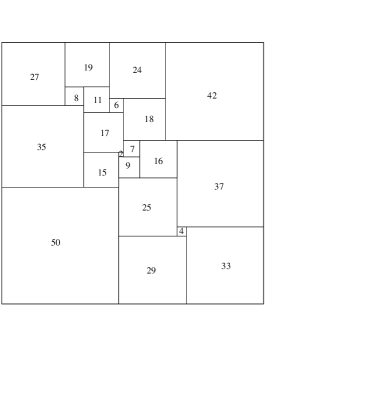
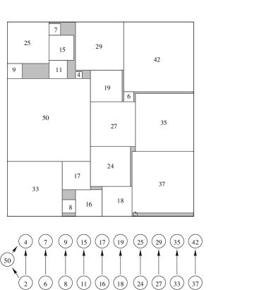
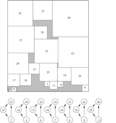
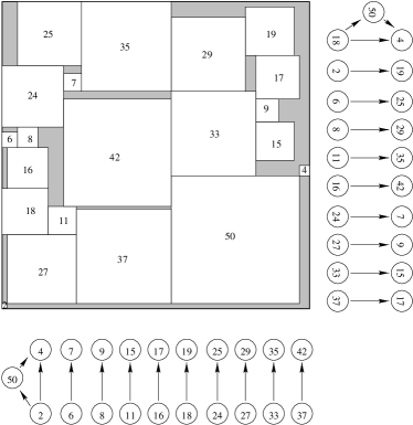
Figure 14: (a) An optimal packing of square21-0 of height 112; (b) an optimal packing of square21-mat of height 117; (c) an optimal packing of square21-tri of height 125; (d) a packing of square21-2mat of size 120x120.

References

- [1] Atmel, AT6000 FPGA configuration guide, Atmel Inc.
- [2] J. E. Beasley, An exact two-dimensional non-guillotine cutting tree search procedure, Operations Research, 33 (1985), pp. 49–64.
- [3] , OR-Library: distributing test problems by electronic mail, Journal of the Operations Research Society, 41 (1990), pp. 1069–1072.
- [4] S. P. Fekete, E. Köhler, and J. Teich, Extending partial suborders, in Electronic Notes in Discrete Mathematics, J. H. Hajo Broersma, Ulrich Faigle and S. Pickl, eds., vol. 8, Elsevier Science Publishers, 2001.
- [5] S. P. Fekete, E. Köhler, and J. Teich, Multi-dimensional packing with order constraints, in Proceedings 7th International Workshop on Algorithms and Data Structures, vol. 2125 of Lecture Notes in Computer Science, Springer-Verlag, 2001, pp. 300–312.
- [6] S. P. Fekete, E. Köhler, and J. Teich, Optimal FPGA module placement with temporal precedence constraints, in Proc. DATE 2001, Design, Automation and Test in Europe, Computer Society Press, 2001, pp. 658–665.
- [7] S. P. Fekete and J. Schepers, An exact algorithm for higher-dimensional orthogonal packing, Operations Research. To appear.
- [8] S. P. Fekete and J. Schepers, A new exact algorithm for general orthogonal d-dimensional knapsack problems, in Algorithms – ESA ’97, vol. 1284, Springer Lecture Notes in Computer Science, 1997, pp. 144–156.
- [9] , New classes of lower bounds for bin packing problems, in Integer Programming and Combinatorial Optimization (IPCO’98), vol. 1412, Springer Lecture Notes in Computer Science, 1998, pp. 257–270.
- [10] , A combinatorial characterization of higher-dimensional orthogonal packing, Mathematics of Operations Research, 29 (2004), pp. 353–368.
- [11] S. P. Fekete and J. Schepers, A general framework for bounds for higher-dimensional orthogonal packing problems, Mathematical Methods of Operations Research, 60 (2004), pp. 311–329.
- [12] P. C. Fishburn, Interval Orders and Interval Graphs, John Wiley & Sons, New York, 1985.
- [13] T. Gallai, Transitiv orientierbare Graphen, Acta Math. Acd. Sci. Hungar., 18 (1967), pp. 25–66.
- [14] A. Ghouilà-Houri, Caractérization des graphes non orientés dont on peut orienter les arrêtes de manière à obtenir le graphe d’une relation d’ordre, C.R. Acad. Sci. Paris, 254 (1962), pp. 1370–1371.
- [15] P. C. Gilmore and A. J. Hoffmann, A characterization of comparability graphs and of interval graphs, Canadian Journal of Mathematics, 16 (1964), pp. 539–548.
- [16] M. C. Golumbic, Algorithmic graph theory and perfect graphs, Academic Press, New York, 1980.
- [17] E. Hadjiconstantinou and N. Christofides, An exact algorithm for general, orthogonal, two-dimensional knapsack problems, European Journal of Operations Research, 83 (1995), pp. 39–56.
- [18] C.-H. Huang and J.-Y. Juang, A partial compaction scheme for processor allocation in hypercube multiprocessors, in Proc. of 1990 Int. Conf. on Parallel Proc., 1990, pp. 211–217.
- [19] D. Kelly, Comparability graphs, in Graphs and Order, I. Rival, ed., D. Reidel Publishing Company, Dordrecht, 1985, pp. 3–40.
- [20] N. Korte and R. Möhring, Transitive orientation of graphs with side constraints, in Proceedings of WG’85, H. Noltemeier, ed., Trauner Verlag, 1985, pp. 143–160.
- [21] , An incremental linear–time algorithm for recognizing interval graphs, Siam Journal of Computing, 18 (1989), pp. 68–81.
- [22] A. Krämer, Scheduling multiprocessor tasks on dedicated processors. Doctoral thesis, Fachbereich Mathematik und Informatik, Universität Osnabrück, 1995.
- [23] E. L. Lawler, J. K. Lenstra, A. H. G. Rinooy Kan, and D. B. Shmoys, Sequencing and scheduling: Algorithms and complexity, in Logistics of Production and Inventory, S. C. Graves, A. H. G. Rinnooy Kan, and P. H. Zipkin, eds., Handbooks in Operations Research and Management, vol. 4, North–Holland, Amsterdam, 1993, pp. 445–522.
- [24] M. Luby, J. Naor, and A. Orda, Tight bounds for dynamic storage allocation, in Proc. 15th ACM-SIAM Sympos. Discrete Algorithms, 1994, pp. 724–732.
- [25] R. H. Möhring, Algorithmic aspects of comparability graphs and interval graphs, in Graphs and Order, I. Rival, ed., D. Reidel Publishing Company, Dordrecht, 1985, pp. 41–101.
- [26] , Algorithmic aspects of the substitution decomposition in optimization over relations, set systems, and Boolean functions, Annals of Oper. Res., 4 (1985/6), pp. 195–225.
- [27] R. H. Möhring, A. S. Schulz, F. Stork, and M. Uetz, Solving project scheduling problems by minimum cut computations, Management Science, 49 (2003), pp. 330–350.
- [28] M. Padberg, Packing small boxes into a big box, Math. Meth. of Op. Res., 52 (2000), pp. 1–21.
- [29] J. Schepers, Exakte Algorithmen für orthogonale Packungsprobleme, Tech. Rep. 97-302, Doctoral thesis, Universität Köln, 1997.
- [30] J. Teich, S. P. Fekete, and J. Schepers, Compile-time optimization of dynamic hardware reconfigurations, in Proc. Int. Conf. on Parallel and Distributed Processing Techniques and Applications (PDPTA’99), Las Vegas, USA, June 1999, pp. 1097–1103.
- [31] J. Teich, S. P. Fekete, and J. Schepers, Optimal hardware reconfiguration techniques, Journal of Supercomputing, 19 (2001), pp. 57–75.
- [32] J. Weglarz, Project Scheduling. Recent Models, Algorithms and Applications, Kluwers Academic Publishers, Norwell, MA, USA, 1999.
- [33] Xilinx, XC6200 field programmable gate arrays, tech. rep., Xilinx, Inc., October 1996.