A Family of Simplified Geometric Distortion Models for Camera Calibration

Abstract

The commonly used radial distortion model for camera calibration is in fact an assumption or a restriction. In practice, camera distortion could happen in a general geometrical manner that is not limited to the radial sense. This paper proposes a simplified geometrical distortion modeling method by using two different radial distortion functions in the two image axes. A family of simplified geometric distortion models is proposed, which are either simple polynomials or the rational functions of polynomials. Analytical geometric undistortion is possible using two of the distortion functions discussed in this paper and their performance can be improved by applying a piecewise fitting idea. Our experimental results show that the geometrical distortion models always perform better than their radial distortion counterparts. Furthermore, the proposed geometric modeling method is more appropriate for cameras whose distortion is not perfectly radially symmetric around the center of distortion.
Key Words: Camera calibration, Radial distortion, Geometric distortion, Geometric undistortion.

I Introduction

For many computer vision applications, such as robot visual inspection and industrial metrology, where a camera is used as a sensor in the system, the camera is usually assumed to be fully calibrated beforehand. Camera calibration is the estimation of a set of parameters that describes the camera’s imaging process. With this set of parameters, a perspective projection matrix can directly link a point in the 3-D world reference frame to its projection (undistorted) on the image plane. This is given by:

$$\lambda\left[\matrix{u\cr v\cr 1}\right]={\bf A}\,\left[{\bf R}\mid{\bf t}\right]\left[\matrix{X^{w}\cr Y^{w}\cr Z^{w}\cr 1}\right]=\left[\matrix{\alpha&\gamma&u_{0}\cr 0&\beta&v_{0}\cr 0&0&1}\right]\left[\matrix{X^{c}\cr Y^{c}\cr Z^{c}}\right],$$ (1)

where $(u,v)$ is the distortion-free image point on the image plane. The matrix $\bf A$ fully depends on the camera’s 5 intrinsic parameters $(\alpha,\gamma,\beta,u_{0},v_{0})$, with $(\alpha,\beta)$ being two scalars in the two image axes, $(u_{0},v_{0})$ the coordinates of the principal point, and $\gamma$ describing the skewness of the two image axes. $[X^{c},Y^{c},Z^{c}]^{T}$ denotes a point in the camera frame that is related to the corresponding point $[X^{w},Y^{w},Z^{w}]^{T}$ in the world reference frame by $P^{c}={\bf R}P^{w}+\bf t$, with $({\bf R},{\bf t})$ being the rotation matrix and the translation vector.

In camera calibration, lens distortion is very important for accurate 3-D measurement [1]. The lens distortion introduces certain amount of nonlinear distortions, denoted by a function $F$ in Fig. 1, to the true image. The observed distorted image thus needs to go through the inverse function $F^{-1}$ to output the corrected image. That is, the goal of lens undistortion, or image correction, is to achieve an overall one-to-one mapping.

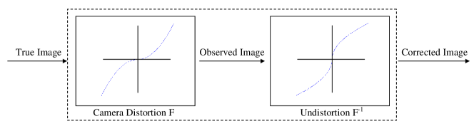
Figure 1: Lens distortion and undistortion.

Among various nonlinear distortions, the radial distortion, which is along the radial direction from the center of distortion, is the most severe part [2, 3]. The removal or alleviation of radial distortion is commonly performed by first applying a parametric radial distortion model, estimating the distortion coefficients, and then correcting the distortion. Most of the existing works on the radial distortion models can be traced back to an early study in photogrammetry [4], where the radial distortion is governed by the following polynomial equation [4, 5, 6, 7]:

$$r_{d}=r+\delta_{r}=r\,f(r,{\bf k})=r\,(1+k_{1}r^{2}+k_{2}r^{4}+k_{3}r^{6}+\cdots),$$ (2)

which is equivalent to

$$x_{d}=x\,f(r,{\bf k}),\;\;y_{d}=y\,f(r,{\bf k}),$$ (3)

where ${\bf k}=[k_{1},k_{2},k_{3},\ldots]$ is a vector of distortion coefficients.

For cameras whose distortion is not perfectly radially symmetric around the center of distortion (which is assumed to be at the principal point in our discussion), radial distortion modeling will not be accurate enough for applications such as precise visual metrology. In this case, a more general distortion model, i.e., geometric distortion, needs to be considered. In this work, a simplified geometric distortion modeling method is proposed, where two different functions in the form of a variety of polynomial and rational functions are used to model the distortions along the two image axes. The proposed simplified geometric distortion models are simpler in structure than that considered in [8] where the total geometric distortion consists of the radial distortion and the decentering distortion. The geometric distortion modeling method proposed is a lumped distortion model that includes all the nonlinear distortion effects.

For real time image processing applications, the property of having analytical undistortion formulae is a desirable feature for both the radial and the geometric distortion models. Though there are ways to approximate the undistortion without numerical iterations, having analytical inverse formulae is advantageous by giving the exact inverse without introducing extra error sources. The key contribution of this paper is the proposition of a family of simplified geometric distortion models that can achieve comparable calibration accuracy to that in [8] and better performance than their radial distortion modeling counterparts. For fairness, these comparisons are based on the same (or reasonable) numbers of distortion coefficients. To preserve the property of having analytical inverse formulae with satisfactory calibration accuracy, a piecewise fitting idea is applied to the simplified geometric modeling for two particular rational distortion functions presented in Sec. II.

The rest of the paper is organized as follows. Sec. II summarizes some existing polynomial and rational radial distortion models that can also be applied to model the geometric distortion. The simplified geometric distortion modeling method is proposed in Sec. III. Experimental results and comparisons between the simplified geometric and the radial distortion models are illustrated and discussed in Sec. IV. Finally, some concluding remarks are given in Sec. V. The variables used throughout this paper are listed in Table I.

TABLE I: List of Variables

Variable	Description
$(u_{d},\,v_{d})$	Distorted image point in pixel
$(u,\,v)$	Distortion-free image point in pixel
$(x_{d},\,y_{d})$	$[x_{d},\,y_{d},\,1]^{T}=A^{-1}[u_{d},\,v_{d},\,1]^{T}$
$(x,\,y)$	$[x,\,y,\,1]^{T}=A^{-1}[u,\,v,\,1]^{T}$
$r_{d}$	$r_{d}^{2}=x_{d}^{2}+y_{d}^{2}$
$r$	$r^{2}=x^{2}+y^{2}$
$\bf k$	Distortion coefficients (radial or geometric)

II Polynomial and Rational Distortion Functions

The commonly used polynomial radial distortion model is given in the form of (2). In this paper, we consider both the polynomial (functions $\#\,1,2,3$ in Table II) and rational radial distortion functions (functions $\#\,5,6,7,8,9,10$ in Table II) [9, 10]. Clearly, all these functions in Table II, except the function $\#4$, are special cases of the following radial distortion function having analytical inverse formulae:

$$f(r,{\bf\kappa})=\frac{1+\kappa_{1}\,r+\kappa_{2}\,r^{2}}{1+\kappa_{3}\,r+\kappa_{4}\,r^{2}+\kappa_{5}\,r^{3}}.$$ (4)

For example, when $\kappa_{1}=0,\kappa_{5}=0$, equation (4) becomes the function $\#10$ in Table II with $k_{1}=\kappa_{2}$, $k_{2}=\kappa_{3}$, and $k_{3}=\kappa_{4}$. Notionwise, $k_{1}$, $k_{2}$, and $k_{3}$ here correspond to their specific distortion function, i.e., $k_{1}$, $k_{2}$, and $k_{3}$ do not have a global meaning. The function $\#4$ in Table II is in the form of (2) with 2 distortion coefficients, which is the most commonly used conventional radial distortion function in the polynomial approximation category. The other 9 functions in Table II are studied specifically with the goal to achieve comparable performance with the function $\#4$ using the least amount of model complexity and as few distortion coefficients as possible. Since the functions $\#9$ and $\#10$ in Table II begin to show comparable calibration performance to the function $\#4$ (as can be seen later in Table III) [10], more complex distortion functions are not studied in this work.

TABLE II: Polynomial and Rational Distortion Functions

$\bf\#$	$f(r,{\bf k})$	$\bf\#$	$f(r,{\bf k})$
1	$1+k_{1}\,r$	6	$1/(1+k_{1}\,r^{2})$
2	$1+k_{1}\,r^{2}$	7	$(1+k_{1}\,r)/(1+k_{2}\,r^{2})$
3	$1+k_{1}\,r+k_{2}\,r^{2}$	8	$1/(1+k_{1}\,r+k_{2}\,r^{2})$
4	$1+k_{1}\,r^{2}+k_{2}\,r^{4}$	9	$(1+k_{1}\,r)/(1+k_{2}\,r+k_{3}\,r^{2})$
5	$1/(1+k_{1}\,r)$	10	$(1+k_{1}\,r^{2})/(1+k_{2}\,r+k_{3}\,r^{2})$

Notice that all the functions in Table II satisfy the following properties:

• The function is radially symmetric around the center of distortion and is expressed in terms of the radius $r$ only;

• The function is continuous and $r_{d}=0$ iff $r=0$;

• The approximation of $x_{d}$ is an odd function of $x$.

The above three properties act as the criteria to be a candidate for the radial distortion function. However, for the general geometric distortion functions, which are not necessarily the same along the two image axes, the first property does not need to be satisfied, though the functions need to be continuous such that there will be no distortion only at the center of distortion.

The well-known radial distortion model (2) that describes the laws governing the radial distortion does not involve a quadratic term. Thus, it might be unexpected to add one. However, when interpreting from the relationship between $(x_{d},y_{d})$ and $(x,y)$ in the camera frame, the purpose of radial distortion function is to approximate the $x_{d}\leftrightarrow x$ relationship, which is intuitively an odd function. Adding a quadratic term to $\delta_{r}$ does not alter this fact as shown in [11]. As demonstrated in [11], it is reasonable to introduce a quadratic term to $\delta_{r}$ to broaden the choice of radial distortion functions with a better calibration fit. Therefore, as long as the above listed three properties are satisfied, there should be no restriction in the form of $\delta_{r}$. With this argument in mind, we also proposed the rational radial distortion models with analytical undistortion formulae as shown in Table II, with details presented in [10].

To compare the performance of the simplified geometric distortion models with their radial distortion counterparts, the calibration procedures presented in [5] are applied. In [5], the estimation of radial distortion is done after having estimated the intrinsic and the extrinsic parameters, just before the nonlinear optimization step. So, for different distortion models (radial or geometric), we can reuse the estimated intrinsic and extrinsic parameters. To compare the performance of different distortion models, the final value of optimization function $J$, which is defined to be [5]:

$$J=\sum_{i=1}^{N}\sum_{j=1}^{n}\|m_{ij}-\hat{m}({\bf A},{\bf k},{\bf R}_{i},{\bf t}_{i},M_{j})\|^{2},$$ (5)

is used, where $\hat{m}({\bf A},{\bf k},{\bf R}_{i},{\bf t}_{i},M_{j})$ is the projection of point $M_{j}$ in the $i^{th}$ image using the estimated parameters, $\bf k$ denotes the distortion coefficients (radial or geometric), $M_{j}$ is the $j^{th}$ 3-D point in the world frame with $Z^{w}=0$, $n$ is the number of feature points in the coplanar calibration object, and $N$ is the number of images taken for calibration.

III Simplified Geometric Distortion Models

III-A Model

A family of simplified geometric distortion models is proposed as

$$x_{d}=x\,f(r,{\bf k}_{1}),\;\;y_{d}=y\,f(r,{\bf k}_{2}),$$ (6)

where the distortion function $f(r,{\bf k})$ in (6) can be chosen to be, though not restricted to, any of the functions in Table II. When ${\bf k}_{1}={\bf k}_{2}={\bf k}$, the geometric distortion reduces to the radial distortion in equation (3). From (6), the relationship between $(u_{d},v_{d})$ and $(u,v)$ becomes

$$\left\{\begin{array}[]{l}u_{d}-u_{0}=(u-u_{0})\,f(r,{\bf k}_{1})\\ \hskip 42.67912pt+\,\gamma/\beta\,(v-v_{0})\,[f(r,{\bf k}_{2})-f(r,{\bf k}_{1})]\\ \hskip 1.70717ptv_{d}-v_{0}=(v-v_{0})\,f(r,{\bf k}_{2})\end{array}\right..$$ (7)

If we define

$$\left\{\begin{array}[]{c}u_{d}-u_{0}=(u-u_{0})\,f(r,{\bf k}_{1})\\ v_{d}-v_{0}=(v-v_{0})\,f(r,{\bf k}_{2})\end{array}\right.,$$ (8)

the relationship between $(x_{d},y_{d})$ and $(x,y)$ becomes

$$\left\{\begin{array}[]{l}x_{d}=x\,f(r,{\bf k}_{1})+\gamma/\alpha\;y\,[f(r,{\bf k}_{1})-f(r,{\bf k}_{2})]\\ y_{d}=y\,f(r,{\bf k}_{2})\end{array}\right..$$ (9)

After nonlinear optimization, the final values of $J$, the intrinsic and extrinsic parameters, and the distortion coefficients using the pair (6), (7) and (8), (9) are extremely close. Thus, in this paper, we only focus on the pair (6), (7), while being aware that similar results can be achieved using (8), (9).

Remark III.1

The distortion models discussed in this paper belong to the category of Undistorted-Distorted model, while the Distorted-Undistorted model also exists in the literature to correct distortion [12]. The idea of simplified geometric distortion modeling can be applied to the D-U formulation simply by defining

$$x=x_{d}\,f(r_{d},{\tilde{\bf k}}_{1}),\;\;y=y_{d}\,f(r_{d},{\tilde{\bf k}}_{2}).$$ (10)

Consistent improvement can be achieved in the above D-U formulation.

In [8], the geometric distortion modeling when written in the U-D formulation is presented as:

$$\left\{\begin{array}[]{l}u_{d}={\bar{u}}\,(1+k_{1}\,r^{2}+k_{2}\,r^{4}+k_{3}\,r^{6}+\cdots)+u_{0}\\ \hskip 22.76219pt\,+(2p_{1}\,{\bar{u}}{\bar{v}}+p_{2}\,(r^{2}+2{\bar{u}}^{2}))(1+p_{3}\,r^{2}+\cdots)\\ v_{d}={\bar{v}}\,(1+k_{1}\,r^{2}+k_{2}\,r^{4}+k_{3}\,r^{6}+\cdots)+v_{0}\\ \hskip 22.76219pt\,+(p_{1}\,(r^{2}+2{\bar{v}}^{2})+2p_{2}\,{\bar{u}}{\bar{v}})(1+p_{3}\,r^{2}+\cdots)\end{array}\right.,$$ (11)

where ${\bar{u}}=u-u_{0},{\bar{v}}=v-v_{0}$. The parameters $(k_{1},k_{2},k_{3})$ are the coefficients for the radial distortion and the parameters $(p_{1},p_{2},p_{3})$ are for the decentering distortion. Compared with (11), the proposed simplified geometric distortion modeling (6), (7) is simpler in the structure and it is a lumped distortion model that includes all the nonlinear distortion effects.

Remark III.2

The two functions that model the distortion in the two image axes are not necessarily of the same form or structure. That is, equation (6) can be extended to have the following more general form

$$x_{d}=x\,f_{x}(r,{\bf k}_{1}),\;\;y_{d}=y\,f_{y}(r,{\bf k}_{2}).$$ (12)

However, since we have no prior information as to how the distortions proceed along the two image axes, model (12) is not investigated in this work for lack of motivation. Of course, by choosing $f_{x}(r,{\bf k}_{1})$ and $f_{y}(r,{\bf k}_{2})$ differently, there is a chance to get an even better result at the expense of making more efforts in figuring out what the best combination should be.

III-B Geometric Undistortion

For the simplified geometric distortion model (6), the property of having analytical undistortion formulae is not preserved for most of the functions in Table II as for the radial distortion. However, when using the function $\#5$ and $\#6$ in Table II, the geometric undistortion can be performed analytically. For example, when

$$f(r,k_{1})=\frac{1}{1+k_{1}r},\;\;f(r,k_{2})=\frac{1}{1+k_{2}r},$$ (13)

from (6), we have

$$x_{d}=x\,\frac{1}{1+k_{1}r},\;\;y_{d}=y\,\frac{1}{1+k_{2}r}.$$ (14)

The geometric undistortion problem is to calculate $(x,y)$ from $(x_{d},y_{d})$ given the distortion coefficients $(k_{1},k_{2})$ that are determined through the nonlinear optimization process. From equation (14), we have the following quadratic function of $r$

$$x_{d}^{2}\,(1+k_{1}\,r)^{2}+y_{d}^{2}\,(1+k_{2}\,r)^{2}=r^{2},$$ (15)

whose analytical solutions exist. The above quadratic function in $r$ has two analytical solutions, where one solution can be discarded because it deviates from $r_{d}$ dramatically. After $r$ is derived, $(x,y)$ can be calculated from $(x_{d},y_{d})$ uniquely. In this way, the geometric undistortion using the function $\#5$ in Table II can be achieved non-iteratively. For the function $\#6$, a similar quadratic function in the form of $x_{d}^{2}\,(1+k_{1}\,{\bar{r}})^{2}+y_{d}^{2}\,(1+k_{2}\,{\bar{r}})^{2}={\bar{r}}$ can be derived with ${\bar{r}}=r^{2}$.

III-C Piecewise Geometric Distortion Models Using Functions $\#5$ and $\#6$ in Table II

For real time image processing applications, geometric distortion models with analytical undistortion formulae are very desirable for the exact inverse. When there is no analytical undistortion formula and to avoid performing the undistortion via numerical iterations, there are ways to approximate the undistortion, such as the model described in [8] for the radial undistortion, where $r$ can be calculated from $r_{d}$ by

$$r=r_{d}\,f(r_{d},-{\bf k}).$$ (16)

The fitting results given by the above model can be satisfactory when the distortion coefficients are small values. However, equation (16) itself introduces additional error that will inevitably degrade the overall calibration accuracy.

The appealing feature of having analytical geometric undistortion formulae when using the functions $\#5$ and $\#6$ in Table II may come with a price. The simple model structure may limit the fitting flexibility and hence the fitting accuracy. In this case, a piecewise fitting idea can be applied to enhance accuracy of the simplified geometric distortion modeling, which is illustrated in Fig. 2 with two segments.

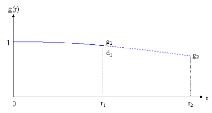
Figure 2: A piecewise continuous function (two-segment).

When using the function $\#5$ in Table II for each segment of $f(r,{\bf k}_{1})$ or $f(r,{\bf k}_{2})$, the two segments are of the form

$$\left\{\begin{array}[]{l}\displaystyle g_{1}(r)=\frac{1}{1+{\bar{k}}_{1}\,r},\;\;\;{\rm for}\;\;r\;\in[0,r_{1}]\\[5.0pt] \displaystyle g_{2}(r)=\frac{1}{a+{\bar{k}}_{2}\,r},\;\;\;{\rm for}\;\;r\;\in(r_{1},r_{2}]\end{array}\right.,$$ (17)

with $r_{1}=r_{2}/2$. To ensure that the overall function (17) is continuous across the interior knot, the following 3 constraints can be applied

$$\frac{1}{1+{\bar{k}}_{1}\,r_{1}}=g_{1},\;\;\frac{1}{a+{\bar{k}}_{2}\,r_{1}}=g_{1},\;\;\frac{1}{a+{\bar{k}}_{2}\,r_{2}}=g_{2},$$ (18)

where $g_{1}=g_{1}(r_{1})=g_{2}(r_{1})$ and $g_{2}=g_{2}(r_{2})$. Since the coefficients $({\bar{k}}_{1},a,{\bar{k}}_{2})$ can be calculated from (18) uniquely by

$$\left\{\begin{array}[]{l}{\bar{k}}_{1}=(1/g_{1}-1)/r_{1}\\ {\bar{k}}_{2}=(1/g_{2}-1/g_{1})/(r_{2}-r_{1})\\ a=1/g_{1}-{\bar{k}}_{2}\,r_{1}\end{array}\right.,$$ (19)

the geometric distortion coefficients that are used in the nonlinear optimization can be chosen to be $(g_{1},g_{2})$ with the initial values $(1,1)$. During the nonlinear optimization process, $({\bar{k}}_{1},a,{\bar{k}}_{2})$ are calculated from $(g_{1},g_{2})$ in each iteration. When using the function $\#6$ in Table II, similar functions to (18) and (19) can be derived by substituting $(r_{1},r_{2})$ with $(r_{1}^{2},r_{2}^{2})$. Furthermore, the piecewise idea can be easily extended to more segments.

When applying the piecewise idea using the functions $\#5$ and $\#6$ in Table II, better calibration accuracy can be achieved yet the property of having analytical geometric undistortion formulae can be retained. The the above feature is clearly at the expense of more segments, i.e., more distortion coefficients to be searched in the optimization process.

IV Experimental Results and Discussions

IV-A Comparison Between the Simplified Geometric and the Radial Distortion Models

Using three groups of test images (the public domain test images [13], the desktop camera images [14] (a color camera), and the ODIS camera images [14, 15] (the camera on the ODIS robot built at Utah State University [16])), the final values of $J$ of the simplified geometric distortion model (6) after nonlinear optimization by the Matlab function fminunc using the 10 functions in Table II are shown in Table III, where the values of $J$ using the same function but under the assumption of the radial distortion are also listed for comparison. In Table III, the numbers 1-10 in the first column denote the 10 functions in Table II in the same order. The extracted corners for the model plane of the desktop and the ODIS cameras are shown in Figs. 3 and 4, where the plotted dots in the center of each square are only used for judging the correspondence with the world reference points.

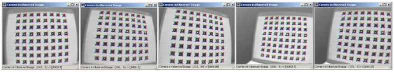
Figure 3: Five images of the model plane with the extracted corners (indicated by cross) for the desktop camera.

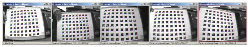
Figure 4: Five images of the model plane with the extracted corners (indicated by cross) for the ODIS camera.

TABLE III: Objective Function $J$ of The Simplified Geometric and The Radial Distortions using the 10 Functions in Table II

	Public Images		Desktop Images		ODIS Images
$\#$	Geometric	Radial	Geometric	Radial	Geometric	Radial
1	180.4617	180.5713	999.6644	1016.7437	928.9073	944.4418
2	148.2608	148.2788	904.0705	904.6796	913.1676	933.0981
3	145.5766	145.6592	801.3148	803.3074	836.9277	851.2619
4	144.8226	144.8802	777.3812	778.9767	825.8771	840.2649
5	184.9429	185.0628	1175.7494	1201.8001	1019.8750	1036.6208
6	146.9811	146.9999	797.9312	798.5720	851.6244	867.6192
7	145.3864	145.4682	786.2204	787.6185	830.6345	845.0206
8	145.3688	145.4504	784.8960	786.3590	829.4675	843.7991
9	144.7560	144.8328	779.0693	780.9060	823.0736	837.9181
10	144.7500	144.8256	777.9869	780.0391	823.2726	838.3245
		144.8179		776.7103		837.7749

From Table III, the values of $J$ of the simplified geometric distortion models are generally smaller than those of the radial distortion models. The improvement for the public and desktop cameras are not significant, while it is significant for the ODIS camera. However, the above comparison between the simplified geometric and the radial distortion models might not be fair since the geometric models have more coefficients and it is evident that each additional coefficient in the model tends to decrease the fitting residual. Due to this concern, the objective function $J$ of the radial distortion modeling using 6 coefficients in equation (2) ($2\times$ the maximal number of coefficients used in the geometric modeling) for the three groups of test images are also shown in the last row of Table III. The reason for choosing the radial distortion model (2) with 6 coefficients is that this model is conventionally used and it is always among the best models in Table II giving the top performance. Again, for the ODIS images, it is observed that the values of $J$ of the geometric modeling are all smaller than that of the radial distortion modeling using 6 coefficients in (2), where the 6 coefficients are $(-0.3601,0.1801,-0.5149,3.1911,-6.4699,4.1625)$, except for the functions $\#1,2,5,6$, which are relatively simple in complexity and have fewer distortion coefficients. It can thus be concluded that the distortion of the ODIS camera is not as perfectly radially symmetric as the other two cameras and the geometric modeling is more appropriate for the ODIS camera.

TABLE IV: Comparisons Between The Simplified Geometric and The Radial Distortion Models for the ODIS Images

Distortion	$\#$	$J$	${\bf k}_{1}$			${\bf k}_{2}$			$\alpha$	$\gamma$	$u_{0}$	$\beta$	$v_{0}$
	1	928.9073	-0.2232	-	-	-0.2413	-	-	272.5073	-0.0784	140.7238	268.7688	115.5717
	2	913.1676	-0.2624	-	-	-0.2890	-	-	256.7545	-0.4848	137.3176	252.4421	117.6516
	3	836.9277	-0.1150	-0.1305	-	-0.1206	-0.1454	-	264.5867	-0.3322	140.4929	260.2474	115.0102
Simplified	4	825.8771	-0.3386	0.1512	-	-0.3718	0.1756	-	259.4480	-0.2434	140.5699	255.2091	114.8777
Geometric	5	1019.8750	0.2679	-	-	0.2968	-	-	275.9477	-0.0049	139.6337	272.7017	117.0080
Distortion	6	851.6244	0.3039	-	-	0.3348	-	-	258.0766	-0.3970	139.5523	253.7985	115.7800
	7	830.6345	-0.0826	0.1964	-	-0.0768	0.2320	-	263.1308	-0.3143	140.6762	258.3793	114.9656
	8	829.4675	0.0736	0.2259	-	0.0685	0.2608	-	262.8587	-0.3068	140.7462	258.1623	114.9220
	9	823.0736	0.9087	0.8695	0.5494	1.6571	1.4811	0.8974	259.5748	-0.2509	140.9331	251.9627	114.7501
	10	823.2726	0.2719	0.0232	0.5950	0.6543	-0.0563	1.1524	260.8910	-0.2444	140.8209	253.8259	114.8106
	1	944.4418	-0.2327	-	-	-	-	-	274.2660	-0.1153	140.3620	268.3070	114.3916
	2	933.0981	-0.2752	-	-	-	-	-	258.3193	-0.5165	137.2150	252.6856	115.9302
	3	851.2619	-0.1192	-0.1365	-	-	-	-	266.0850	-0.3677	139.9198	260.3133	113.2412
	4	840.2649	-0.3554	0.1633	-	-	-	-	260.7658	-0.2741	140.0581	255.1489	113.1727
Radial	5	1036.6208	0.2828	-	-	-	-	-	278.0218	-0.0289	139.5948	271.9274	116.2992
Distortion	6	867.6192	0.3190	-	-	-	-	-	259.4947	-0.4301	139.1252	253.8698	113.9611
	7	845.0206	-0.0815	0.2119	-	-	-	-	264.4038	-0.3505	140.0528	258.6809	113.1445
	8	843.7991	0.0725	0.2419	-	-	-	-	264.1341	-0.3429	140.1092	258.4206	113.1129
	9	837.9181	1.2859	1.1839	0.7187	-	-	-	259.2880	-0.2824	140.2936	253.7043	113.0078
	10	838.3245	0.4494	-0.0124	0.8540	-	-	-	260.9370	-0.2804	140.2437	255.3178	113.0561

Figure 5 shows the undistorted image points for the third image in Fig. 4 using the simplified geometric distortion model $\#4$ and the radial distortion model (2) with 6 coefficients. The difference between the undistorted image points using the above two models can be observed at the image boundary (the enlarged plots of region₁ and region₂ are shown in Fig. 6), which is quite significant for applications that require sub-pixel accuracy.

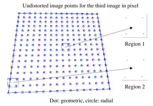
Figure 5: Undistorted image points for the third image in Fig. 4 using the simplified geometric distortion model $\#4$ and the radial distortion model (2) with 6 coefficients.

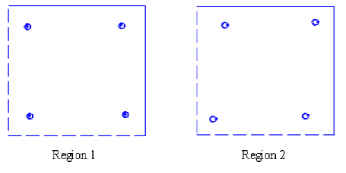
Figure 6: Enlarged plot of the two regions in Fig. 5.

The detailed estimated parameters using the 10 functions in Table II for the simplified geometric and the radial distortion models are shown in Table IV using the ODIS images, where the 5 intrinsic parameters are also listed for showing the consistency. Furthermore, the values of $J$ of the radial and geometric distortion models are plotted in Fig. 7 for the ODIS images, where the $x$ axis denotes the sorted model numbers in Table II in an order with $J$ decreasing monotonously.

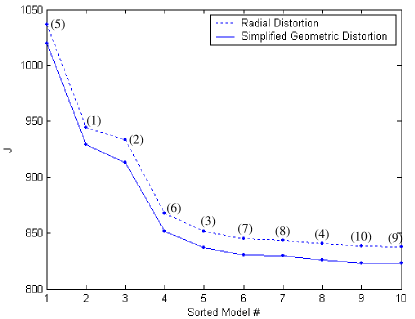
Figure 7: Objective function $J$ of the simplified geometric and the radial distortion models for the ODIS images using the 10 functions in Table II (corresponding model numbers are shown in the text).

From Table IV, it is observed that the distortion coefficients ${\bf k}$ for the radial distortion models always lie between the corresponding values of ${\bf k}_{1}$ and ${\bf k}_{2}$ for the simplified geometric distortion models. Due to this reason, the resultant $f(r,{\bf k})$ curves also lie between the $f(r,{\bf k}_{1})$ and $f(r,{\bf k}_{2})$ curves, which can be seen from Fig. 8, where the $f(r,{\bf k})$, $f(r,{\bf k}_{1})$, and $f(r,{\bf k}_{2})$ curves for the ODIS images using the third function in Table II (referred to as Model₃ hereafter) are plotted as an example. It can thus be concluded that when using one $f(r,{\bf k})$, it tries to find a compromise between $f(r,{\bf k}_{1})$ and $f(r,{\bf k}_{2})$.

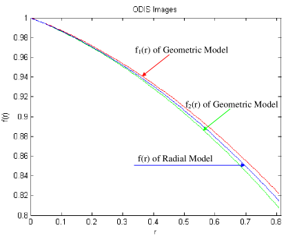
Figure 8: $f(r,{\bf k}_{1})$ and $f(r,{\bf k}_{2})$ vs. $f(r,{\bf k})$ for the ODIS images using Model₃.

From Fig. 8, the difference between $f(r,{\bf k}_{1})$ and $f(r,{\bf k}_{2})$ increases as $r$ increases, which is barely noticeable at $r=0.1$ but begins to be observable at $r=0.3$. This information can also be seen from Fig. 9, where the relationship between $(x,y)$ and $(x_{d},y_{d})$ is plotted for the ODIS images using Model₃. When using two different functions to model the distortion along the two image axes, the distortion shown in Fig. 9 is not exactly a smaller circle (since ${\bf k_{1}}<{\bf 0}$ and ${\bf k}_{2}<{\bf 0}$), but a wide ellipse that is slightly shorter in the $y$ direction.

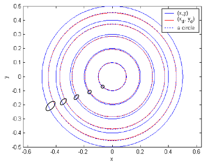
Figure 9: $(x_{d},y_{d})$ vs. $(x,y)$ for the ODIS images under the simplified geometric distortion assumption using Model₃.

Remark IV.1

Classical criteria that are used in the computer vision to assess the accuracy of calibration includes the radial distortion [17]. However, to our best knowledge, there is not a systematically quantitative and universally accepted criterion in the literature for performance comparisons among different distortion models. Due to this lack of criterion, in our work, the comparison is based on, but not restricted to, the fitting residual of the full-scale nonlinear optimization in (5).

IV-B Comparison Between the Simplified Geometric and the Piecewise Geometric Distortion Models using Functions $\#5$ and $\#6$ in Table II

Using the ODIS images, the final values of $J$ for the 1-segment, 2-segment, and 3-segment piecewise rational geometric distortion models using the functions $\#5$ and $\#6$ in Table II are shown in Table V, where $f(r,{\bf k}_{1})$ and $f(r,{\bf k}_{2})$ have 1, 2, or 3 components depending on the number of segments used. The maximal range of $r$ is listed in the last column for each case. From Table V, it is observed that the values of $J$ after applying the piecewise idea are always smaller than those using fewer segments. A careful comparison between the values of $J$ of the 3-segment piecewise geometric distortion modeling using the function $\#6$ in Table V and the simplified geometric distortion models in Table III shows that the 3-segment piecewise geometric modeling using the function $\#6$ can have fairly good results. The piecewise idea is thus more suitable for applications that require real time image undistortion.

TABLE V: Comparisons Between The Geometric and The Piecewise Geometric Distortion Models

Distortion	Images	$\#$	$J$	$f(r,{\bf k}_{1})$ Values			$f(r,{\bf k}_{2})$ Values			$r_{\rm max}$
		5	147.8709	0.9960	0.9830	0.9651	0.9957	0.9825	0.9646	0.4252
3-Segment	Public	6	144.9397	0.9957	0.9830	0.9646	0.9952	0.9825	0.9640	0.4260
Geometric		5	802.8802	0.9699	0.8954	0.8047	0.9666	0.8957	0.8048	0.8643
Distortion	Desktop	6	782.3082	0.9726	0.8980	0.8069	0.9712	0.8991	0.8088	0.8673
		5	840.2963	0.9657	0.9035	0.8284	0.9720	0.9022	0.8234	0.8167
	ODIS	6	823.8911	0.9709	0.9084	0.8327	0.9741	0.9044	0.8253	0.8182
		5	149.5355	0.9871	0.9630	-	0.9862	0.9622	-	0.4250
2-Segment	Public	6	145.7634	0.9902	0.9639	-	0.9895	0.9634	-	0.4263
Geometric		5	824.7348	0.9167	0.7949	-	0.9168	0.7996	-	0.8612
Distortion	Desktop	6	787.4081	0.9380	0.8027	-	0.9391	0.8064	-	0.8665
		5	850.6158	0.9249	0.8242	-	0.9197	0.8107	-	0.8101
	ODIS	6	830.7617	0.9449	0.8313	-	0.9405	0.8182	-	0.8176
		5	184.9428	0.9587	-	-	0.9580	-	-	0.4216
Single	Public	6	146.9811	0.9642	-	-	0.9640	-	-	0.4264
Geometric		5	1175.6975	0.7983	-	-	0.8149	-	-	0.7968
Distortion	Desktop	6	797.9354	0.8033	-	-	0.8057	-	-	0.8654
		5	1019.8751	0.8261	-	-	0.8109	-	-	0.7852
	ODIS	6	851.6577	0.8331	-	-	0.8191	-	-	0.8119

The resulting estimated $f(r,{\bf k}_{1})$ and $f(r,{\bf k}_{2})$ curves of the 2-segment and 3-segment geometric distortion models using the rational function $\#6$ in Table II for the ODIS images are plotted in Figs. 10 and 11.

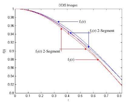
Figure 10: $f(r)$ curves of the 2-segment and the single rational geometric distortion models using function $\#6$ in Table II for the ODIS images.

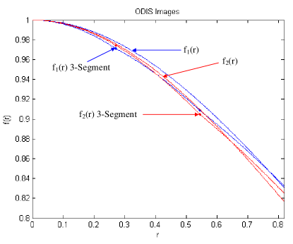
Figure 11: $f(r)$ curves of the 3-segment and the single rational geometric distortion models using function $\#6$ in Table II for the ODIS images.

One issue in the implementation of the piecewise idea is how to decide $r_{\rm max}$, which is related to the estimated extrinsic parameters that are changing from iteration to iteration during the nonlinear optimization process. In our implementation, for each camera, 5 images are taken. $r_{\rm max}$ is chosen to be the maximum $r$ of all the extracted feature points on the 5 images for each iteration.

IV-C Comparison Between the Geometric Modeling Methods (6) and (11)

Both using 6 coefficients, the values of $J$ of the simplified geometric distortion modeling method (6) using function $f(r)=1+k_{1}r^{2}+k_{2}r^{4}+k_{3}r^{6}$ are shown in Table VI for the three groups of test images, where $J$ of the geometric modeling method (11) in [8] with the distortion coefficients $(k_{1},k_{2},k_{3},p_{1},p_{2},p_{3})$ is also listed for comparison. From Table VI, it is observed that the simplified geometric modeling method, though simpler in structure, does not necessarily give a less accurate calibration performance.

TABLE VI: Comparison Between The Geometric Distortion Modeling Methods (6) and (11)

Eqn.	Public Images	Desktop Images	ODIS Images
(6)	144.7596	775.9196	823.9299
(11)	142.9723	772.8905	834.5090

Remark IV.2

To make the results in this paper reproducible by other researchers for further investigation, we present the options we use for the nonlinear optimization: options = optimset(‘Display’, ‘iter’, ‘LargeScale’, ‘off’, ‘MaxFunEvals’, 8000, ‘TolX’, $10^{-5}$, ‘TolFun’, $10^{-5}$, ‘MaxIter’, 120). The raw data of the extracted feature locations in the image plane are also available [14].

V Concluding Remarks

In this paper, a family of simplified geometric distortion models are proposed that apply different polynomial and rational functions along the two image axes. Experimental results are presented to show that the proposed simplified geometric distortion modeling method can be more appropriate for cameras whose distortion is not perfectly radially symmetric around the center of distortion. Analytical geometric undistortion is possible using two of the distortion functions discussed in this paper and their performance can be improved by applying a piecewise idea.

The proposed simplified geometric distortion modeling method is simpler than that in [8], where the nonlinear geometric distortion is further classified into the radial distortion and the decentering distortion and the total distortion is a sum of these distortion effects. Though simple in the structure, the simplified geometric distortion modeling gives comparable performance to that in [8]. Furthermore, for some cameras, like the ODIS camera studied here, the simplified geometric distortion modeling can even perform better.

In this paper, we are restricting the maximal number of distortion coefficients considered to be 3 in all the distortion functions in Table II, because it has also been found that too high an order may cause numerical instability [3, 5, 18]. However, the appropriate number of distortion coefficients should not be determined only by a numerical issue. A stronger argument should come from the relationship between $J$ and the number of distortion coefficients. The appropriate number of distortion coefficients is chosen when the calibration accuracy does not show to have much improvement as the number of distortion coefficients increases beyond this value.

The comparison between the piecewise and the simplified geometric distortion models in Sec. IV-B brings up the question of preference between “more segments with low-complexity function” or “more distortion coefficients with more complex function”. The above question is not answered in this work and is a direction of future investigation.

References

- [1] Reimar K. Lenz and Roger Y. Tsai, “Techniques for calibration of the scale factor and image center for high accuracy 3-D machine vision metrology,” IEEE Transactions on Pattern Analysis and Machine Intelligence, vol. 10, no. 5, pp. 713–720, Sep. 1988.
- [2] Frederic Devernay and Olivier Faugeras, “Straight lines have to be straight,” Machine Vision and Applications, vol. 13, no. 1, pp. 14–24, 2001.
- [3] Roger Y. Tsai, “A versatile camera calibration technique for high-accuracy 3D machine vision metrology using off-the-shelf TV cameras and lenses,” IEEE Journal of Robotics and Automation, vol. 3, no. 4, pp. 323–344, Aug. 1987.
- [4] Chester C Slama, Ed., Manual of Photogrammetry, American Society of Photogrammetry, fourth edition, 1980.
- [5] Zhengyou Zhang, “Flexible camera calibration by viewing a plane from unknown orientation,” IEEE International Conference on Computer Vision, pp. 666–673, Sep. 1999.
- [6] J. Heikkil and O. Silvn, “A four-step camera calibration procedure with implicit image correction,” in IEEE Computer Society Conference on Computer Vision and Pattern Recognition, San Juan, Puerto Rico, 1997, pp. 1106–1112.
- [7] Janne Heikkila and Olli Silven, “Calibration procedure for short focal length off-the-shelf CCD cameras,” in Proceedings of 13th International Conference on Pattern Recognition, Vienna, Austria, 1996, pp. 166–170.
- [8] Janne Heikkila, “Geometric camera calibration using circular control points,” IEEE Transactions on Pattern Analysis and Machine Intelligence, vol. 22, no. 10, pp. 1066–1077, Oct. 2000.
- [9] Richard Hartley and Andrew Zisserman, Multiple View Geometry, Cambridge University Press, 2000.
- [10] Lili Ma, YangQuan Chen, and Kevin L. Moore, “Rational radial distortion models with analytical undistortion formulae,” Submitted for Journal Publication, http://arxiv.org/abs/cs.CV/0307047, 2003.
- [11] Lili Ma, YangQuan Chen, and Kevin L. Moore, “Flexible camera calibration using a new analytical radial undistortion formula with application to mobile robot localization,” in IEEE International Symposium on Intelligent Control, Houston, USA, Oct. 2003.
- [12] Toru Tamaki, Tsuyoshi Yamamura, and Noboru Ohnishi, “Unified approach to image distortion,” in International Conference on Pattern Recognition, Aug. 2002, pp. 584–587.
- [13] Zhengyou Zhang, “Experimental data and result for camera calibration,” Microsoft Research Technical Report, http://rese- arch.microsoft.com/~zhang/calib/, 1998.
- [14] Lili Ma, “Camera calibration: a USU implementation,” CSOIS Technical Report, ECE Department, Utah State University, http://arXiv.org/abs/cs.CV/0307072, May, 2002.
- [15] “Cm3000-l29 color board camera (ODIS camera) specification sheet,” http://www.video-surveillance-hidden-spy -cameras.com/cm3000l29.htm.
- [16] Lili Ma, Matthew Berkemeier, YangQuan Chen, Morgan Davidson, and Vikas Bahl, “Wireless visual servoing for ODIS: an under car inspection mobile robot,” in Proceedings of the 15th IFAC Congress. IFA, 2002, pp. 21–26.
- [17] Juyang Weng, Paul Cohen, and Marc Herniou, “Camera calibration with distortion models and accuracy evaluation,” IEEE Transactions on Pattern Analysis and Machine Intelligence, vol. 14, no. 10, pp. 965–980, Oct. 1992.
- [18] G. Wei and S. Ma, “Implicit and explicit camera calibration: theory and experiments,” IEEE Transactions on Pattern Analysis and Machine Intelligence, vol. 16, no. 5, pp. 469–480, May 1994.