Quantifying and Visualizing Attribute Interactions:
An Approach Based on Entropy

Abstract

Interactions are patterns between several attributes in data that cannot be inferred from any subset of these attributes. While mutual information is a well-established approach to evaluating the interactions between two attributes, we surveyed its generalizations as to quantify interactions between several attributes. We have chosen McGill’s interaction information, which has been independently rediscovered a number of times under various names in various disciplines, because of its many intuitively appealing properties. We apply interaction information to visually present the most important interactions of the data. Visualization of interactions has provided insight into the structure of data on a number of domains, identifying redundant attributes and opportunities for constructing new features, discovering unexpected regularities in data, and have helped during construction of predictive models; we illustrate the methods on numerous examples. A machine learning method that disregards interactions may get caught in two traps: myopia is caused by learning algorithms assuming independence in spite of interactions, whereas fragmentation arises from assuming an interaction in spite of independence.

Keywords: Interaction, Dependence, Mutual Information, Interaction Information, Information Visualization

1 Introduction

One of the basic notions in probability is the concept of independence. Binary events $a$ and $b$ are independent if and only if $P(a,b)=P(a)P(b)$. Independence also implies that $a$ is irrelevant to $b$. However, independence is not a stable relation: $a$ may become dependent with $b$ if we observe another event $c$. For example, define $c$ to happen when $a$ and $b$ take place together ($a\wedge b$), or do not take place together ($\neg a\wedge\neg b$). Even if $a$ and $b$ are independent and random, they become dependent in the context of $c$. Alternatively, $a$ may become independent of $b$ in the context of $c$, even if they were dependent before: imagine that $a$ and $b$ are two independently sampled uncertain measurements of $c$. Without $c$, the measurements are similar, hence their dependence. With the knowledge of $c$, however, the similarity between $a$ and $b$ disappears. It is hence difficult to systematically investigate dependencies.

Conditional independence was proposed as a solution to the above problem of flickering dependencies. Events $a$ and $b$ are conditionally independent with respect to event $c$ if and only if they are independent in the context of every outcome of $c$. In probability theory, this can be expressed as $P(a|b,c)=P(a|c)$. Hence, independence cannot be claimed unless it has been verified in the context of all other events. This helps us simplify the model of the environment.

In this text, we endorse a different type of regularities, interactions, which subsumes conditional independence. An interaction is a regularity, a pattern, a dependence present only in the whole set of events, but not in any subset. When there is such a regularity, we say that the attributes of the set interact. For example, a 2-way interaction between two events indicates that the joint probability distribution cannot be described with the assumption of mutual independence between events. A 3-way interaction between three events is equivalent to the inability to describe the joint probability distribution with any marginalization, it is hence necessary to model it directly. Interactions are local, meaning that they are only defined in the context of events they relate to. Interactions are stable, because introduction of newly observed events cannot change the interactions that already exist among the events. An interaction is unambiguous, meaning that there is only one way of describing it. Interactions are symmetric and undirected, so directionality no longer needs to be explained by, e.g., causality.

The contributions of each successive section of this paper can be summarized as follows:

• A survey of information-based measures of interaction among attributes.

• Several novel diagrams for visualization of interactions in the data.

• Investigation of relevance of interactions in the context of supervised machine learning.

2 Quantifying Interactions with Entropy

In this section, we will revise the basic concepts of information theory in order to derive interaction information, our proposal for quantifying higher-order dependencies in data. Interaction information captures and quantifies the earlier intuitive view of probabilistic interactions. The interdisciplinary review of related work at the end of the section shows that virtually the same formulae have emerged independently a number of times in various disciplines, ranging from physics to psychology, adding weight to the worth of the idea.

2.1 Attributes, Probabilities and Entropy

While we used the terminology of events earlier, we will now migrate to common machine learning terminology. An attribute $A$ will be considered to be a collection of independent but mutually exclusive events, or attribute values, $\{a_{1},a_{2},a_{3},\ldots,a_{n}\}$. We will consider $a$ as an example of an event from $A$’s alphabet, or $A$’s value. Variates, random variables, communication sources and classifiers can all be considered to be types of attributes. In machine learning, an instance corresponds to another event, which is described as a set of attributes’ events. For example, an instance is “Dancing in cold weather, in rain and in wind.” and such instances are described with four attributes, $A$ with the alphabet or range $\Re_{A}=\{\text{dancing},\neg\text{dancing}\}$, $B:\Re_{B}=\{\text{cold},\text{cool},\text{warm},\text{hot}\}$, $C:\{\text{rain},\text{cloud},\text{clear}\}$, and $D:\{\text{calm},\text{breeze},\text{wind}\}$. If our task is deciding whether to dance or not to dance, attribute $A$ is the label.

An instance is a synchronous observation of the attributes, and we can describe the relationships between the attributes, assuming that the instances are permutable, with a joint probability distribution $P(A,B,C)$. Marginal probability distributions are projections of the joint where we disregard but a subset of attributes, for example:

$$P(A)=P(A,\cdot,\cdot)=\sum_{b\in\Re_{B}}\sum_{c\in\Re_{C}}P(A,b,c).$$

The essence of learning is simplification of the joint probability distributions, achieved by exploiting certain regularities. A very useful discovery is that $A$ and $B$ are independent, meaning that $P(A,B)$ can be approximated with $P(A)P(B)$. If so, we say that $A$ and $B$ do not 2-interact, or that there is no 2-way interaction between $A$ and $B$. Unfortunately, attribute $C$ may affect the relationship between $A$ and $B$ in a number of ways. Controlling for the value of $C$, $A$ and $B$ may prove to be dependent even if they were previously independent. Or, $A$ and $B$ may actually be independent when controlling for $C$, but dependent otherwise.

If the introduction of the third attribute $C$ affects the dependence between $A$ and $B$, we say that $A$, $B$ and $C$ 3-interact, meaning that we cannot decipher their relationship without considering all of them at once. An appearance of a dependence is an example of a positive interaction: positive interactions imply that the introduction of the new attribute increased the amount of dependence. A disappearance of a dependence is a kind of a negative interaction: negative interactions imply that the introduction of the new attribute decreased the amount of dependence. If $C$ does not affect the dependence between $A$ and $B$, we say that there is no 3-interaction.

There are plenty of real-world examples of interactions. Negative interactions imply redundance. For example, weather attributes rain and lightning are dependent, because they occur together. But the attribute storm interacts negatively with them, since it reduces their dependence. Storm explains a part of their dependence. Should we wonder whether there is lightning, the information that there is rain would contribute no information if we already knew that there is a storm.

Positive interactions imply synergy instead. For example, employment of a person and criminal behavior are not particularly dependent attributes (most unemployed people are not criminals, and many criminals are employed), but adding the knowledge of whether the person has a new sports car suddenly makes these two attributes dependent: it is a lot more frequent that an unemployed person has a new sports car if he is involved in criminal behavior; the opposite is also true: it is somewhat unlikely that an unemployed person will have a new sports car if he is not involved in criminal behavior.

In real life, it is quite rare to have perfectly positive or perfectly negative interactions. Instead, we would like to quantify the magnitude and the type of an interaction. For this, we will employ entropy as a measure of uncertainty. A measure of mutual dependence can be constructed from an uncertainty measure, defining dependence as the amount of shared uncertainty.

Let us assume an attribute, $A$. Shannon’s entropy measured in bits is a measure of unpredictability of an attribute (Shannon, 1948):

$$H(A)\triangleq-\sum_{a\in\Re_{A}}P(a)\log_{2}{P(a)}$$ (1)

By definition, $0\log_{2}0=0$. The higher the entropy, the less reliable are our predictions about $A$. We can understand $H(A)$ as the amount of uncertainty about $A$, as estimated from its probability distribution. Although this definition is appropriate only for discrete sources, or discretized continuous sources, Shannon (1948) also presents a direct definition for continuous ones.

2.2 Entropy Calculus for Two Attributes

Let us now introduce a new attribute, $B$. We have observed the joint probability distribution, $P(A,B)$. We are interested in predicting $A$ with the knowledge of $B$. At each value of $B$, we observe the probability distribution of $A$, and this is expressed as a conditional probability distribution, $P(A|B)$. Conditional entropy, $H(A|B)$, quantifies the remaining uncertainty about $A$ with the knowledge of $B$:

$$H(A|B)\triangleq-\sum_{a\in\Re_{A},b\in\Re_{B}}{P(a,b)\log_{2}{P(a|b)}}=H(A,B)-H(B)$$ (2)

We quantify the 2-way interaction between two attributes with mutual information:

$$\begin{split}I(A;B)\triangleq\sum_{a\in\Re_{A},b\in\Re_{B}}{P(a,b)\log_{2}\frac{P(a,b)}{P(a)P(b)}}=H(A)+H(B)-H(A,B)\\ =H(A)-H(A|B)=I(B;A)=H(B)-H(B|A)\end{split}$$ (3)

In essence, $I(A;B)$ is a measure of correlation between attributes, which is always zero or positive. It is zero if and only if the two attributes are independent, when $P(A,B)=P(A)P(B)$. Observe that the mutual information between attributes is the average mutual information between events in attributes’ alphabets. If $A$ is an attribute and $L$ is the label attribute, $I(A;L)$ measures the amount of information provided by $A$ about $L$: in this context it is often called information gain.

A 2-way interaction helps reduce our uncertainty about either of the two attributes with the knowledge of the other one. We can calculate the amount of uncertainty remaining about the value of $A$ after introducing knowledge about the value of $B$. This remaining uncertainty is $H(A|B)$, and we can obtain it using mutual information, $H(A|B)=H(A)-I(A;B).$ Sometimes it is worth expressing it as a percentage, something that we will refer to as relative mutual information. For example, after introducing attribute $B$, we have $100\%\cdot H(A|B)/H(A)$ percent of uncertainty about $A$ remaining. For two attributes, the above notions are illustrated in Fig. 1.

Figure 1: A graphical illustration of the relationships between information-theoretic measures of the joint distribution of attributes $A$ and $B$. The surface area of a section corresponds to the labelled quantity. This illustration is inspired by Cover and Thomas (1991).

2.3 Entropy Calculus for Three Attributes

Let us now introduce the third attribute, $C$. We could wonder how much uncertainty about $A$ remains after having obtained the knowledge of $B$ and $C$: $H(A|BC)=H(ABC)-H(BC).$ We might also be interested in seeing how $C$ affects the interaction between $A$ and $B$. This notion is captured with conditional mutual information:

$$\begin{split}I(A;B|C)\triangleq\sum_{a,b,c}{P(a,b,c)\log_{2}\frac{P(a,b|c)}{P(a|c)P(b|c)}}=H(A|C)+H(B|C)-H(AB|C)\\ =H(A|C)-H(A|B,C)=H(AC)+H(BC)-H(C)-H(ABC).\end{split}$$ (4)

Conditional mutual information is always positive or zero; when it is zero, it means that $A$ and $B$ are unrelated given the knowledge of $C$, or that $C$ completely explains the association between $A$ and $B$. From this, it is sometimes inferred that $A$ and $B$ are both consequences of $C$. If $A$ and $B$ are conditionally independent, we can apply the naïve Bayesian classifier for predicting $C$ on the basis of $A$ and $B$ with no remorse. Conditional mutual information is a frequently used heuristic for constructing Bayesian networks (Cheng et al., 2002).

Conditional mutual information $I(A;B|C)$ describes the relationship between $A$ and $B$ in the context of $C$, but we do not know the amount of influence resulting from the introduction of $C$. This is achieved by the measure of the intersection of all three attributes, or interaction information (McGill, 1954) or McGill’s multiple mutual information (Han, 1980):

$$\begin{split}I(A;B;C)\triangleq I(A;B|C)-I(A;B)=I(A,B;C)-I(A;C)-I(B;C)\\ =H(AB)+H(BC)+H(AC)-H(A)-H(B)-H(C)-H(ABC).\end{split}$$ (5)

Interaction information among attributes can be understood as the amount of information that is common to all the attributes, but not present in any subset. Like mutual information, interaction information is symmetric, meaning that $I(A;B;C)=I(A;C;B)=I(C;B;A)=\ldots$. Since interaction information may be negative, we will often refer to the absolute value of interaction information as interaction magnitude. Again, be warned that interaction information among attributes is the average interaction information among the corresponding events.

The concept of total correlation (Watanabe, 1960) describes the total amount of dependence among the attributes:

$$\begin{split}C(A,B,C)\triangleq H(A)+H(B)+H(C)-H(ABC)\\ =I(A;B)+I(B;C)+I(A;C)+I(A;B;C).\end{split}$$ (6)

It is always positive, or zero if and only if all the attributes are independent, $P(A,B,C)=P(A)P(B)P(C)$. However, it will not be zero even if only a pair of attributes are dependent. For example, if $P(A,B,C)=P(A,B)P(C)$, the total correlation will be non-zero, but only $A$ and $B$ are dependent. Hence, it is not justified to claim an interaction among all three attributes. For such a situation, interaction information will be zero, because $I(A;B|C)=I(A;B)$.

2.3.1 Positive and negative interactions

Interaction information can either be positive or negative. Perhaps the best way of illustrating the difference is through the equivalence $I(A;B;C)=I(A,B;C)-I(A;C)-I(B;C)$: Assume that we are uncertain about the value of $C$, but we have information about $A$ and $B$. Knowledge of $A$ alone eliminates $I(A;C)$ bits of uncertainty from $C$. Knowledge of $B$ alone eliminates $I(B;C)$ bits of uncertainty from $C$. However, the joint knowledge of $A$ and $B$ eliminates $I(A,B;C)$ bits of uncertainty. Hence, if interaction information is positive, we benefit from a synergy. A well-known example of such synergy is the exclusive or: $C=A+B\pmod{2}$. If interaction information is negative, we suffer diminishing returns by several attributes providing overlapping, redundant information. Another interpretation, offered by McGill (1954), is as follows: Interaction information is the amount of information gained (or lost) in transmission by controlling one attribute when the other attributes are already known.

2.3.2 Interactions and Supervised Learning

The objective of unsupervised machine learning is the construction of a model which helps predict the value of any attribute with partial knowledge of other attribute values. For attributes $A,B,C$, unsupervised models approximate the joint probability distribution $P(A,B,C)$ with a joint probability distribution function $\hat{P}(A,B,C)$. On the other hand, the objective of supervised learning is to predict the distinguished label attribute with the (partial) knowledge of other attributes. Supervised models attempt to describe the conditional probability distribution, distinguishing the label $C$ from ordinary attributes $A$ and $B$. The conditional probability distribution can be modelled with informative models $\hat{P}(A,B|C)$, or with discriminative models $\hat{P}(C|A,B)$ (Rubinstein and Hastie, 1997). For example, the naïve Bayesian classifier is an informative model, while logistic regression is a discriminative model.

In supervised learning we are primarily interested in interactions that involve the label: interactions between non-label attributes alone are rarely investigated. In fact, only interactions involving the label can provide any information about it. If there is no interaction with the label, there is no information about the label. As an example, we formulate the naïve Bayesian classifier as an approximation to the Bayes rule, introducing the assumption that $A$ and $B$ are independent given $C$, $P(A,B|C)\approx P(A|C)P(B|C)$:

$$P(C|A,B)=P(C)\frac{P(A,B|C)}{P(A,B)}\approx P(C)\frac{P(A|C)P(B|C)}{P(A,B)}$$ (7)

The conditional independence assumption is that there does not exist any value of $C$, in the context of which $A$ and $B$ would 2-interact. We will refer to this type of interactions as informative conditional interactions, the interactions in informative probability distributions. For a label $C$ and attributes $X$ and $Y$, the 2-way informative conditional interaction information is $I(X;Y|C)$, the familiar conditional mutual information. It can be seen as the expected 2-way informative conditional interaction information between $A$ and $B$ over the values of $C$.

The relationship between the ordinary and the informative conditional interactions is easily seen from the definition of 3-way interaction information in (5): it is the difference between the two kinds of 2-way interaction information. It is quite easy to see that when $I(A;B|C)=0$, the 3-way interaction information can only be nonnegative. When the 3-way interaction information is positive, the 2-way conditional interaction information must also be positive. However, when the 3-way interaction information is zero or negative, no specific conclusions can be made about the 2-way informative conditional interaction.

2.3.3 Limitations of the Bayesian network representation of conditional independence relations

Given three attributes, if any pair of attributes is conditionally independent given the third, e.g., $I(A;B|C)=0$, the interaction information among the three cannot be positive. Such a situation can be perfectly represented with a Bayesian network (Pearl, 1988): $A\leftarrow C\rightarrow B$. If a pair of attributes are mutually independent, for example $I(A;B)=0$, the interaction information, if it exists, can only be positive. Such an interaction can also be perfectly described with a Bayesian network, $A\rightarrow C\leftarrow B$.

Unfortunately, there are situations that can be described by several Bayesian networks, none of which is able to describe the structure of interactions. Assume the exclusive or problem, where $A=B+C\pmod{2}$ with binary attributes. The mutual information between any pair of attributes is zero, yet the attributes are in a 3-way interaction. We can formally describe this with three consistent Bayesian networks: $A\rightarrow C\leftarrow B,$ $A\rightarrow B\leftarrow C$ and $B\rightarrow A\leftarrow C$, but no network emphasizes the fact that there are no 2-way interactions. The interaction information in this case, however, is strictly positive.

Another example is the case of triplicated attributes, $A=B=C$. In this case, for all combinations of attributes, the conditional mutual information is zero. On the other hand, every pair of attributes is deterministically 2-way interacting. Again, the fact cannot be seen from any of the Bayesian networks consistent with the data: $A\leftarrow C\rightarrow B$, $A\leftarrow B\rightarrow C$ and $B\leftarrow A\rightarrow C$. The interaction information in this case is strictly negative.

These two were extreme examples, but having zero conditional mutual information is too an extreme example. Conditional or mutual information is rarely zero, yet some are larger than others. The larger they are the more likely it is that the dependencies are not coincidental, and the more information we gain by not ignoring them. We quantify interactions for this precise reason, and our visualization methods emphasize the quantified interaction magnitude.

2.4 Quantifying $n$-Way Interactions

In this section, we will generalize the above concepts to interactions involving an arbitrary number of attributes. Assume a set of attributes ${\cal A}=\{X_{1},X_{2},\ldots,X_{n}\}$. Each attribute $X\in{\cal A}$ has an alphabet $\Re_{X}=\{x_{1},x_{2},\ldots,x_{p}\}$. If we consider the whole set of attributes ${\cal A}$ as a multivariate or a vector of attributes, we have a joint probability distribution, $P(\mathchoice{\mbox{\boldmath$\displaystyle\mathbf{a}$}}{\mbox{\boldmath$\textstyle\mathbf{a}$}}{\mbox{\boldmath$\scriptstyle\mathbf{a}$}}{\mbox{\boldmath$\scriptscriptstyle\mathbf{a}$}})$. $\Re_{\mathchoice{\mbox{\boldmath$\displaystyle\mathbf{A}$}}{\mbox{\boldmath$\textstyle\mathbf{A}$}}{\mbox{\boldmath$\scriptstyle\mathbf{A}$}}{\mbox{\boldmath$\scriptscriptstyle\mathbf{A}$}}}$ is the Cartesian product of individual attributes’ alphabets, $\Re_{\mathchoice{\mbox{\boldmath$\displaystyle\mathbf{A}$}}{\mbox{\boldmath$\textstyle\mathbf{A}$}}{\mbox{\boldmath$\scriptstyle\mathbf{A}$}}{\mbox{\boldmath$\scriptscriptstyle\mathbf{A}$}}}=\Re_{X_{1}}\times\Re_{X_{2}}\times\cdots\times\Re_{X_{n}}$, and $\mathchoice{\mbox{\boldmath$\displaystyle\mathbf{a}$}}{\mbox{\boldmath$\textstyle\mathbf{a}$}}{\mbox{\boldmath$\scriptstyle\mathbf{a}$}}{\mbox{\boldmath$\scriptscriptstyle\mathbf{a}$}}\in\Re_{\mathchoice{\mbox{\boldmath$\displaystyle\mathbf{A}$}}{\mbox{\boldmath$\textstyle\mathbf{A}$}}{\mbox{\boldmath$\scriptstyle\mathbf{A}$}}{\mbox{\boldmath$\scriptscriptstyle\mathbf{A}$}}}$. We can then define a marginal probability distribution for a subset of attributes ${\cal S}\subseteq{\cal A}$, where ${\cal S}=\{X_{i(1)},X_{i(2)},\ldots,X_{i(k)}\}$:

$$P(\mathchoice{\mbox{\boldmath$\displaystyle\mathbf{s}$}}{\mbox{\boldmath$\textstyle\mathbf{s}$}}{\mbox{\boldmath$\scriptstyle\mathbf{s}$}}{\mbox{\boldmath$\scriptscriptstyle\mathbf{s}$}})\triangleq\sum_{\begin{subarray}{c}\mathchoice{\mbox{\boldmath$\displaystyle\mathbf{a}$}}{\mbox{\boldmath$\textstyle\mathbf{a}$}}{\mbox{\boldmath$\scriptstyle\mathbf{a}$}}{\mbox{\boldmath$\scriptscriptstyle\mathbf{a}$}}\in\Re_{\mathchoice{\mbox{\boldmath$\displaystyle\mathbf{A}$}}{\mbox{\boldmath$\textstyle\mathbf{A}$}}{\mbox{\boldmath$\scriptstyle\mathbf{A}$}}{\mbox{\boldmath$\scriptscriptstyle\mathbf{A}$}}},\\ \mathchoice{\mbox{\boldmath$\displaystyle\mathbf{s}$}}{\mbox{\boldmath$\textstyle\mathbf{s}$}}{\mbox{\boldmath$\scriptstyle\mathbf{s}$}}{\mbox{\boldmath$\scriptscriptstyle\mathbf{s}$}}_{j}=\mathchoice{\mbox{\boldmath$\displaystyle\mathbf{a}$}}{\mbox{\boldmath$\textstyle\mathbf{a}$}}{\mbox{\boldmath$\scriptstyle\mathbf{a}$}}{\mbox{\boldmath$\scriptscriptstyle\mathbf{a}$}}_{i(j)},\\ j=1,2,\ldots,k\end{subarray}}P(\mathchoice{\mbox{\boldmath$\displaystyle\mathbf{a}$}}{\mbox{\boldmath$\textstyle\mathbf{a}$}}{\mbox{\boldmath$\scriptstyle\mathbf{a}$}}{\mbox{\boldmath$\scriptscriptstyle\mathbf{a}$}}).$$ (8)

Next, we can define the entropy for a subset of attributes:

$$H({\cal S})\triangleq-\sum_{\mathchoice{\mbox{\boldmath$\displaystyle\mathbf{v}$}}{\mbox{\boldmath$\textstyle\mathbf{v}$}}{\mbox{\boldmath$\scriptstyle\mathbf{v}$}}{\mbox{\boldmath$\scriptscriptstyle\mathbf{v}$}}\in\mathchoice{\mbox{\boldmath$\displaystyle\mathbf{\cal S}$}}{\mbox{\boldmath$\textstyle\mathbf{\cal S}$}}{\mbox{\boldmath$\scriptstyle\mathbf{\cal S}$}}{\mbox{\boldmath$\scriptscriptstyle\mathbf{\cal S}$}}}P(\mathchoice{\mbox{\boldmath$\displaystyle\mathbf{v}$}}{\mbox{\boldmath$\textstyle\mathbf{v}$}}{\mbox{\boldmath$\scriptstyle\mathbf{v}$}}{\mbox{\boldmath$\scriptscriptstyle\mathbf{v}$}})\log_{2}{P(\mathchoice{\mbox{\boldmath$\displaystyle\mathbf{v}$}}{\mbox{\boldmath$\textstyle\mathbf{v}$}}{\mbox{\boldmath$\scriptstyle\mathbf{v}$}}{\mbox{\boldmath$\scriptscriptstyle\mathbf{v}$}})}$$ (9)

We define $k$-way interaction information by generalizing from formulae in (McGill, 1954) for $k=3,4$ to an arbitrary $k$:

$$I({\cal S})\triangleq-\sum_{{\cal T}\subseteq{\cal S}}{(-1)^{|{\cal S}|-|{\cal T}|}H({\cal T})}=I({\cal S}\setminus X|X)-I({\cal S}\setminus X),\,X\in{\cal S},$$ (10)

$k$-way multiple mutual information is closely related to the lattice-theoretic derivation of multiple mutual information (Han, 1980), $\Delta h({\cal S})=-I({\cal S})$, and to the set-theoretic derivation of multiple mutual information (Yeung, 1991) and co-information (Bell, 2003) as $I^{\prime}({\cal S})=(-1)^{|{\cal S}|}I({\cal S})$.

Finally, we define $k$-way total correlation as (Watanabe, 1960, Han, 1980):

$$C({\cal S})\triangleq\sum_{X\in{\cal S}}H(X)-H({\cal S})=\sum_{{\cal T}\subseteq{\cal S},|{\cal T}|\geq 2}{I({\cal T})}.$$ (11)

We can see that it is possible to arrive at an estimate of total correlation by summing all the interaction information existing in the model. Interaction information can hence be seen as a decomposition of a $k$-way dependence into a sum of $l,\,l\leq k$ dependencies.

2.5 Related Work

Although the idea of mutual information has been formulated (as ‘rate of transmission’) already by Shannon (1948), the seminal work on higher-order interaction information was done by McGill (1954), with application to the analysis of contingency table data collected in psychometric experiments, trying to identify multi-way dependencies between a number of variables. The analogy between variables and information theory was derived from viewing each variable as an information source. These concepts have also appeared in biology at about the same time, as Quastler (1953) gave the same definition of interaction information as McGill, but with a different sign. The concept of interaction information was also discussed in early textbooks on information theory (e.g. Fano, 1961). A formally rigorous study of interaction information was a series of papers by Han, the best starting point to which is (Han, 1980). A further discussion of mathematical properties of positive versus negative interactions appeared in (Tsujishita, 1995). Bell (2003) discussed the concept of co-information, closely related to the Yeung’s notion of multiple mutual information, and suggested its usefulness in the context of dependent component analysis.

In physics, Cerf and Adami (1997) associated positive interaction information of three variables (referred to as ternary mutual information) with the non-separability of a system in quantum physics. Matsuda (2000) applied interaction information (referred to as higher-order mutual information) and the positive/negative interaction dichotomy to the study of many-body correlation effects in physics, and pointed out an analogy between interaction information and Kirkwood superposition approximation. In ecology, Orlóci et al. (2002) referred to interaction information as ‘the mutual portion of total diversity’ and denoted it as $I(ABC)$. In the field of neuroscience, Brenner et al. (2000) noted the utility of interaction information for three attributes, which they referred to as synergy. They used interaction information for observing relationships between neurons. Gat (1999) referred to positive interactions as synergy, while and to negative interactions as redundance. The concept of interactions also appeared in cooperative game theory with applications in economics and law. The issue is observation of utility of cooperation to different players, for example, a coalition is an interaction between players which might either be of negative or positive value for them. Grabisch and Roubens (1999) formulated the Banzhaf interaction index, which proves to be a generalization of interaction information, if negative entropy is understood as game-theoretic value, attributes as players, and all other players are disregarded while evaluating a coalition of a subset of them (Jakulin, 2003). Gediga and Düntsch (2003) applied these notions to rough set analysis.

The topic of interactions was a topic of extensive investigation in statistics, and our review will be an extremely limited one. Darroch (1974) surveyed two definitions of interactions, the multiplicative, which was introduced by Bartlett (1935) and generalized by Roy and Kastenbaum (1956), and the additive definition due to Lancaster (1969). Darroch (1974) preferred the multiplicative definition, and described a ‘partition’ of interaction which is equivalent to the entropy-based approach described in this paper. Other types of partitioning were discussed by Lancaster (1969), and more recently by Amari (2001) in the context of information geometry.

Watanabe (1960) was one of the first to discuss total correlation in detail, even if the same concept had been described (but not named) previously by McGill (1954). Paluš (1994) refers to it as redundancy. Studenỳ and Vejnarovà (1998) investigated the properties of conditional mutual information as applied to conditional independence models. They discussed total correlation, generalized it, and named it multiinformation. Multiinformation was used to show that conditional independence models have no finite axiomatic characterization. More recently Wennekers and Ay (2003) have referred to total correlation as stochastic interaction, and Sporns et al. (2000) as integration. Chechik et al. (2002) investigated the similarity between total correlation and interaction information. Vedral (2002) has compared total correlation with interaction information in the context of quantum information theory. Total correlation is sometimes even referred to as multi-variate mutual information (Boes and Meyer, 1999).

2.5.1 The relationship between set theory and entropy

Interaction information is similar to the notion of intersection of three sets. It has been long known that these computations resemble the inclusion-exclusion properties of set theory Yeung (1991). We can view mutual information $(;)$ as a set-theoretic intersection $(\cap)$, joint entropy $(,)$ as a set-theoretic union $(\cup)$ and conditioning $(|)$ as a set difference $(-)$. The notion of entropy or information corresponds to $\mu$, a signed measure of a set, which is a set-additive function. Yeung defines $\mu$ to be an I-measure, where $\mu^{\ast}$ of a set is equal the entropy of the corresponding probability distribution, for example $\mu^{\ast}(\tilde{X})=H(X)$. Yeung refers to diagrammatic representations of a set of attributes as information diagrams, similar to Venn diagrams. Some think that using these diagrams for more than two information sources is misleading (MacKay, 2003), for example because the set measures can be negative, because there is no clear concept of what the elements of the sets are, and because it is not always possible to keep the surface areas proportional to the actual uncertainty.

Through the principle of inclusion-exclusion and understanding that multiple mutual information is equivalent to an intersection of sets, it is possible to arrive to a slightly different formulation of interaction information (e.g. Yeung, 1991). This formulation is the most frequent in recent literature, but it has a counter-intuitive semantics, as illustrated by Bell (2003): $n$-parity, a special case of which is the XOR problem for $n=2$, is an example of a purely $n$-way dependence. It has a positive co-information when $n$ is even, and a negative co-information when $n$ is odd. For that reason we decided to adopt the original definition of (McGill, 1954).

2.5.2 Testing the significance of dependencies and interactions

McGill (1954) discussed that expressions involving entropy are closely associated with likelihood ratio; total correlation and conditional mutual information follow a $\chi^{2}$ distribution for large samples. Han (1980) also discussed asymptotic properties of interaction information. Entropy is a general statistic, useful for ascertaining significance of various forms of dependence or independence among attributes.

2.5.3 Total and partial correlation

Entropy is just a specific approach to quantification of variance, and the inferences we make have much in common with those based upon partial correlation. Our visualization methods would be equally suitable for presenting partial correlation among continuous variables.

Partial correlation quantifies the amount of variance in the dependent variable explained by only one independent variable, controlling for a set of other independent variables (Yule, 1907). If correlation can be seen as a measure of dependence between a dependent variable and an independent variable, multiple correlation as a measure of dependence between a dependent variable and a number of independent variables, we can understand partial correlation as a quantification of conditional dependence for continuous variables.

Venn diagrams, such as the one in Fig. 1 are also an item of interest in statistics, where multiple correlation or the $R^{2}$ or $\eta^{2}$ statistics represents the total amount of variance in the dependent variable explained in the sample data by the independent variables. With this index, it is too possible to render Venn diagrams representing shared variance, even if these indices do not have properties as appealing as entropy.

3 Visualizing Interactions

Interactions among attributes are often very interesting for a human analyst (Freitas, 2001). We will propose a number of novel diagrams in this section to visually present interactions in data, providing examples of quantification of interactions. Visualization methods attempt to present the most important interactions that exist in the data. Entropy and interaction information yield easily to graphical presentation, as they are both measured in bits. Nonetheless, all the visualization methods could be easily used with the measures of interaction magnitude. The optimal type of visualization method depends on the type of learning it supports. In unsupervised learning, we are interested in general relationships between attributes. In supervised learning, we are particularly interested in the relevance of individual attributes to predictions about the label.

In our analysis, we have used the ‘census/adult’, ‘mushroom’, ‘pima’, ‘zoo’, ‘Reuters-21578’ and ‘German credit’ data sets from the UCI repository (Hettich and Bay, 1999). In all cases, maximum likelihood joint probability estimates were used. On sparse data, smoothing the probability estimates is a good idea (Good, 1965); we recommend multinomial probability estimation with Dirichlet priors, a special case of which is Laplace’s law of succession; alternatively, for distributions following the power law, such as word frequencies, Good-Turing smoothing is more appropriate.

3.1 Unsupervised Visualization

We can illustrate the interaction quantities we discussed with information graphs, introduced in (Jakulin, 2003) as interaction diagrams. They are inspired by Venn diagrams, which we render as an ordinary graph, while the surface area of each node identifies the amount of uncertainty. They can also be seen as quantified factor graphs (Kschischang et al., 2001).

White circles indicate the positive ‘information’ of the model, the entropy eliminated by the joint model. Gray circles indicate the two types of negative ‘entropy’, the initial uncertainty of the attributes and the negative interactions indicating the redundancies. Redundancies can be interpreted as overlapping of information, while information is overlapping of entropy. The joint entropy of the attributes, or any subset of them, is obtained by summing all the gray nodes and subtracting all the white nodes linked to the relevant attributes.

We start with a simple example involving two attributes from the ‘census/adult’ data set, illustrated in Fig. 2. The instances of the data set are a sample of adult population from a census database.

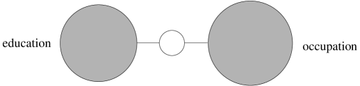
Figure 2: Education and occupation do have something in common: the area of the white circle indicates that the mutual information $I(\text{education};\text{occupation})$ is non-zero. This is a 2-way interaction, since two attributes are involved in it. The areas of the gray circles quantify entropy of individual attributes: $H(\text{education})$ and $H(\text{occupation})$.

The occupation is slightly harder to predict a priori than the education because occupation entropy is larger. Because the amount of mutual information is fixed, the knowledge about the occupation will eliminate a larger proportion of uncertainty about the level of education than vice versa, but there is no reason for asserting directionality merely from the data, especially as such predictive directionality could be mistaken for causality.

3.1.1 A negative interaction

The relationship between three characteristics of animals in the ‘zoo’ database is rendered in Fig. 3. All three attributes are 2-interacting, but there is an overlap in the mutual information among each pair, indicated by a negative interaction information. It is illustrated as the gray circle, connected to the 2-way interactions, which means that they have a shared quantity of information. It would be wrong to subtract all the 2-way interactions from the sum of individual entropies to estimate the complexity of the triplet, as we would underestimate it. For that reason, the 3-way negative interaction acts as a correcting factor.

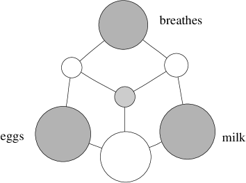
Figure 3: An example of a 3-way negative interaction between the properties ‘lays eggs?’, ‘breathes?’ and ‘has milk?’ for different animals.

This model is also applicable to supervised learning. If we were interested if an animal breathes, but knowing whether it gives milk and whether it lays eggs, we would obtain the residual uncertainty $H(\text{breathes}|\text{eggs},\text{milk})$ by the following formula:

$$H(\text{breathes})-\left(I(\text{breathes};\text{eggs})+I(\text{breathes};\text{milk})+I(\text{breathes};\text{eggs};\text{milk})\right).$$

This domain is better predictable than the one from Fig. 2, since the 2-way interactions are comparable in size to the prior attribute entropies. It is quite easy to see that knowing whether whether an animal lays eggs provides us pretty much all the evidence whether it has milk: mammals do not lay eggs. Of course, such deterministic rules are not common in natural domains.

Furthermore, the 2-way interactions between breathing and eggs and between breathing and milk are very similar in magnitude to the 3-way interaction, but opposite in sign, meaning that they cancel each other out. Using the relationship between conditional mutual information and interaction information from (5), we can conclude that:

$$I(\text{breathes};\text{eggs}|\text{milk})\approx 0$$

$$I(\text{breathes};\text{milk}|\text{eggs})\approx 0$$

Therefore, if the 2-way interaction between such a pair is ignored, we need no 3-way correcting factor. The relationship between these attributes can be described with two Bayesian networks models, each assuming that a certain 2-way interaction does not exist in the context of the remaining attribute:

$$\text{breathes}\leftarrow\text{milk}\rightarrow\text{eggs}$$

$$\text{breathes}\leftarrow\text{eggs}\rightarrow\text{milk}$$

If we were using the naïve Bayesian classifier for predicting whether an animal breathes, we might also find out that feature selection could eliminate one of the attributes: Trying to decide whether an animal breathes, and knowing that the animal lays eggs, most of the information contributed by the fact that the animal doesn’t have milk is redundant. Of course, during classification we might have to classify an animal only with the knowledge of whether it has milk, because the egg-laying attribute value is missing: this problem is rarely a concern in feature selection and feature weighting.

3.1.2 A positive interaction

Most real-life domains are difficult, meaning that it is hopeless trying to predict the outcome deterministically. One such problem domain is a potential customer’s credit risk estimation. Still, we can do a good job predicting the changes in risk for different attribute values. The ‘German credit’ domain describes credit risk for a number of customers. Fig. 4 describes a relationship between the risk with a customer and two of his characteristics. The mutual information between any attribute pairs is low, indicating high uncertainty and weak predictability. The interesting aspect is the positive 3-interaction, which additionally reduces the entropy of the model. We emphasize the positivity by painting the circle corresponding to the 3-way interaction white, as this indicates information.

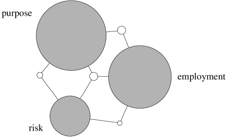
Figure 4: An example of a 3-way positive interaction between the customer’s credit risk, his purpose for applying for a credit and his employment status.

It is not hard to understand the significance of this synergy. On average, unemployed applicants are riskier as customers than employed ones. Also, applying for a credit to finance a business is riskier than applying for a TV set purchase. But if we heard that an unemployed person is applying for a credit to finance purchasing a new car, it would provide much more information about risk than if an employed person had given the same purpose. The corresponding reduction in credit risk uncertainty is the sum of all three interactions connected to it, on the basis of employment, on the basis of purpose, and on the basis of employment and purpose simultaneously.

It is extremely important to note that the positive interaction coexists with a mutual information between both attributes. If we removed one of the attributes because it is correlated with the other one in a feature selection procedure, we would also give up the positive interaction. In fact, positively interacting attributes are often correlated.

3.1.3 Interactions with zero interaction information

The first explanation for a situation with zero 3-way interaction information is that an attribute $C$ does not affect the relationship between attributes $A$ and $B$, thus explaining the zero interaction information $I(A;B|C)=I(A;B)\Rightarrow I(A;B;C)=0$. A homogeneous association among three attributes is described by all the attributes 2-interacting, but not 3-interacting. This would mean that their relationship is fully described by a loopy set of 2-way marginal associations. Although one could imagine that Fig. 5 describes such a homogeneous association, there is another possibility.

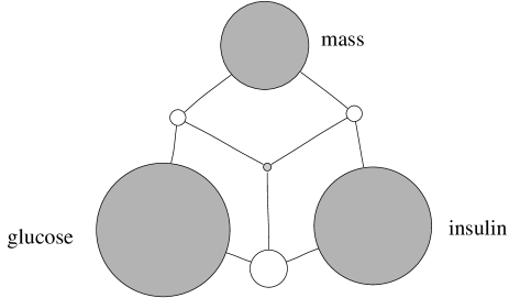
Figure 5: An example of an approximately homogeneous association between body mass, and insulin and glucose levels in the ‘pima’ data set. All the attributes are involved in 2-way interactions, yet the negative 3-way interaction is very weak, indicating that all the 2-way interactions are independent. An alternative explanation would be a mixture of a positive and a negative interaction.

Imagine a situation which is a mixture of a positive and a negative interaction. Three attributes $A,B,C$ take values from $\{0,1,2\}$. The permissible events are $\{e_{1}:A=B+C\pmod{2},\,e_{2}:A=B=C=2\}$. The event $e_{1}$ is the familiar XOR problem, denoting a positive interaction. The event $e_{2}$ is an example of perfectly correlated attributes, an example of a negative interaction. In an appropriate probabilistic mixture, for example $\text{Pr}\{e_{1}\}\approx 0.773,\,\text{Pr}\{e_{2}\}\approx 0.227$, the interaction information $I(A;B;C)$ approaches zero. Namely, $I(A;B;C)$ is the average interaction information across all the possible combinations of values of $A,B$ and $C$. The distinctly positive interaction for the event $e_{1}$ is cancelled out, on average, with the distinctly negative interaction for the event $e_{2}$. The benefit of joining the three attributes and solving the XOR problem exactly matches the loss caused by duplicating the dependence between the three attributes.

Hence, 3-way interaction information should not be seen as a full description of the 3-way interaction but as the interaction information averaged over the attribute values, even if we consider interaction information of lower and higher orders. These problems are not specific only to situations with zero interaction information, but in general. If a single attribute contains information about complex events, much information is blended together, which should rather be kept apart. Not to be misled by such mixtures, we may represent a many-valued attribute $A$ with a set of binary attributes, each corresponding to one of the values of $A$. Alternatively, we may examine the value of interaction information at particular attribute values. The visualization procedure may assist in determining the interactions to be examined closely by including bounds or confidence intervals for interaction information across all combinations of attribute values; when the bounds are not tight, a mixture can be suspected.

3.1.4 Interaction patterns in data

If the number of attributes under investigation is increased, the combinatorial complexity of interaction information may quickly get out of control. Fortunately, interaction information is often low for most combinations of unrelated attributes. We have also observed that the average interaction information of a certain order is decreasing with the order in a set of attributes. A simple approach is to identify $N$ interactions with maximum interaction magnitude among the $n$. For performance and reliability, we also limit the maximum interaction order to $k$, meaning that we only investigate $l$-way interactions, $2\leq l\leq k\leq n$. Namely, it is difficult to reliably estimate joint probability distributions of high order. The estimate of $P(X)$ is usually more robust than the estimate of $P(X,Y,Z,W)$ given the same number of instances.

Mediation and moderation

A larger scale information graph with a selection of interactions in the ‘mushroom’ domain is illustrated in Fig. 6. Because edibility is the attribute of interest (the label), we center our attention on it, and display a few other attributes associated with it. The informativeness of the stalk shape attribute towards mushroom’s edibility is very weak, but this attribute has a massive synergistic effect if accompanied with the stalk root shape attribute. We can describe the situation with the term moderation (Baron and Kenny, 1986): stalk shape ‘moderates’ the effect of stalk root shape on edibility. Stalk shape is hence a moderator variable. It is easy to see that such a situation is problematic for feature selection: if our objective was to predict edibility, a myopic feature selection algorithm would eliminate the stalk shape attribute, before we could take advantage of it in company of stalk root shape attribute. Because the magnitude of the mutual information between edibility and stalk root shape is similar in magnitude to the negative interaction among all three, we can conclude that there is a conditional independence between edibility of a mushroom and its stalk root shape given the mushroom’s odor. A useful term for such a situation is mediation (Baron and Kenny, 1986): odor ‘mediates’ the effect of stalk root shape on edibility.

The 4-way interaction information involving all four attributes was omitted from the graph, but it is distinctly negative. This can be understood by looking at the information gained about edibility from the other attributes and their interactions with the actual entropy of edibility: we cannot explain 120% of entropy, unless we are counting the evidence twice. The negativity of the 4-way interaction indicates that a certain amount of information provided by the stalk shape, stalk root shape and their interaction is also provided by the odor attribute.

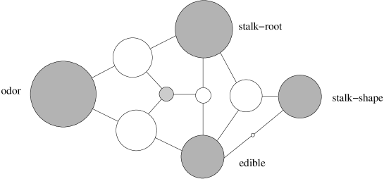
Figure 6: A selection of several important interactions in the ‘mushroom’ domain.

Synonymy and polysemy

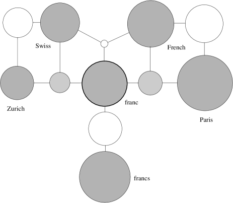
Figure 7: A selection of interactions involving the keyword ‘franc’ in news reports shows that interaction analysis can help identify useful contexts, synonyms and polysemy in information retrieval.

In complex data sets, such as the ones for information retrieval, the number of attributes may be measured in tens of thousands. Interaction analysis must hence stem from a particular reference point. For example, let us focus on the keyword ‘franc’, the currency, in the ‘Reuters’ data set. This keyword is not a label, but merely a determiner of context. We investigate the words that co-appear with it in news reports, and identify a few that are involved in 2-way interactions with it. Among these, we may identify those of the 3-way interactions with high normed interaction magnitude. The result of this analysis is rendered in Fig. 7. We can observe the positive interaction among ‘Swiss’, ‘French’ and ‘franc’ which indicates that ‘franc’ is polysemous. There are two contexts in which the word ‘franc’ appears, but these two contexts do not mix, and this causes the interaction to be positive. The strong 2-way interaction between ‘franc’ and ‘francs’ indicates a likelihood of synonymy: the two words are frequently both present or both absent, and the same is true of pairs ‘French’-‘Paris’ and ‘Swiss’-‘Zurich’. Looking at the mutual information (which is not illustrated), the two negative interactions are in fact near conditional independencies, where ‘Zurich’ and ‘franc’ are conditionally independent given ‘Swiss’, while ‘French’ and ‘franc’ are conditionally independent given ‘Paris’. Hence, the two keywords that are best suited to distinguish the contexts of the kinds of ‘franc’ are ‘Swiss’ and ‘Paris’. These tree are positively interacting, too.

3.2 Supervised Visualization

The objective of supervised learning is acquiring information about a particular label attribute from the other attributes in the domain. In such circumstances, we are interested only in those relationships between attributes that involve the label. Figuratively, we place ourselves into the label and view the other attributes from this perspective. It enables us to simplify the earlier diagrams considerably, which, in turn, facilitates application of interaction analysis methodology to exploratory data analysis.

There are several types of inter-attribute relationships which can be of interest. Interaction graphs (Jakulin and Bratko, 2003) disclose 2-way and 3-way interactions involving the label in a domain. Interaction dendrograms (Jakulin et al., 2003) are a compact summary of proximity between attributes with respect to the similarity (or synergy) of the information they provide about the label. Conditional interaction graphs attempt to illustrate the magnitude of unwanted dependencies which affect the performance in learning algorithms that make the conditional independence assumption.

3.2.1 Interaction dendrograms

In initial phases of exploratory data analysis, we might not be interested in detailed relationships between attributes, but merely wish to discover groups of mutually interacting attributes. In supervised learning, we are not investigating the relationships between attributes themselves (where mutual information would have been the metric of interest), but rather the relationships between the mutual information of either attribute with the label. In other words, we would like to know whether two attributes provide similar information about the label, or whether there is synergy between attributes’ information about the label.

To perform any kind of similarity-based analysis, we should define a similarity or a dissimilarity measure between attributes. With respect to the amount of interaction, interacting attributes should appear close to one another, and non-interacting attributes far from one another. One of the most frequently used similarity measures for clustering is Jaccard’s coefficient (Jaccard, 1908). For two sets, $\cal A$ and $\cal B$, the Jaccard’s coefficient (along with several other similarity measures) can be expressed through set cardinality (Manning and Schütze, 1999):

$$J({\cal A},{\cal B})\triangleq\frac{\left|{\cal A}\cap{\cal B}\right|}{\left|{\cal A}\cup{\cal B}\right|}$$ (12)

If we understand interaction information as a way of measuring the cardinality of the intersection in Fig. 1 and in Section. 2.5.1, where mutual information corresponds to the intersection, and joint entropy as the union, we can define the normed mutual information between attributes $A$ and $B$:

$$\|I(A,B)\|\triangleq\frac{I(A;B)}{H(A,B)}$$ (13)

Màntaras’ distance $d_{M}$ (López de Màntaras, 1991), which has been shown to be a useful heuristic for feature selection, less sensitive to the attribute alphabet size, is closely related to normed mutual information: $d_{M}(A,B)=1-\|I(A,B)\|$. Dividing by the joint entropy helps us reduce the effect of the number of attribute values, hence facilitating comparisons of mutual information between different attributes. Rajski’s distance (Rajski, 1961) is identical to $d_{M}$, but predates it, while normed mutual information is identical to interdependence redundancy (Wong and Liu, 1975).

To present the attribute information similarities to a human analyst, we may tabulate it in a dissimilarity matrix, where color may code the interaction information magnitude and interaction type. Such matrices may become unwieldy with a large number of attributes. To summarize them, we employ the techniques of clustering or multi-dimensional scaling. For visualizing higher-order interactions in an analogous way, we can introduce a further attribute $C$ either as context, using normed conditional mutual information $\|I(A,B|C)\|\triangleq I(A;B|C)/H(A,B|C)$, or as another attribute in interaction information by using normed interaction magnitude:

$$\|I(A,B,C)\|_{+}\triangleq\frac{\left|I(A;B;C)\right|}{H(A,B,C)},$$ (14)

where the interaction magnitude $\left|I(A;B;C)\right|$ is the absolute value of interaction information. $C$ has to be fixed and usually corresponds to the label, while $A$ and $B$ are variables that iterate across all combinations of remaining attributes.

Figure 8: An interaction dendrogram illustrates which attributes interact, positively or negatively, with the label in the ‘census/adult’ data set. The label indicates the individual’s salary. The number of asterisks indicates the amount of mutual information between an attribute and the label.

In the example in Fig. 8, we used Ward’s method for agglomerative hierarchical clustering for summarizing the attribute similarity matrix of normed interaction magnitude $\|I(A,B,C)\|_{+}$ for every pair of attributes $A,B$ and the fixed label $C$. Since the clustering algorithm worked with dissimilarities rather than with similarities, we took the reciprocal value of the normed interaction magnitude, and set an upper limit of dissimilarity (e.g., $K=1000$) to prevent independent attributes from disproportionately affecting the graphical representation.

The resulting interaction dendrogram is one approach to variable clustering, where the proximity is based on the redundancy or synergy of the attributes’ information about the label. We can observe that there are two distinct clusters of attributes. One cluster contains attributes related to the lifestyle of the person: age, family, working hours, sex. The second cluster contains attributes related to the occupation and education of the person. The third cluster is not compact, and contains the information about the native country, race and work class, all relatively uninformative about the label.

Normed interaction magnitude helps identify the groups of attributes that should be investigated more closely. We can use color to convey the type of the interaction. For example, we color zero interactions green, positive interactions red and negative interactions blue, mixing all three color components depending on the normed interaction information. Blue clusters indicate on average negatively interacting groups, and red clusters indicate positively interacting groups of attributes.

Interaction dendrograms may be useful for feature selection. The fnlwgt and race attributes in Fig. 8 do not participate in any positive interactions, and are uninformative by themselves: they are natural candidates for elimination during feature selection. On the other hand, each cluster of negatively interacting attributes has a considerable amount of redundance. For example, older people tend to be married, and highly educated people have spent many years in school. In aggressive feature selection, we could hence simply pick the individually best attributes from each cluster. In our example, these would be marital status and education.

3.2.2 Interaction graphs

Many interesting relationships are not visible in detail in the dendrogram. To drill deeper into the relationships among a group of attributes, we can apply interaction graphs. There, individual attributes are represented as graph nodes and a selection of the 3-way interactions as edges. To limit the complexity arising from a combinatorial explosion of the number of interactions in a domain with many attributes, we restrict the number of interactions illustrated only to those with the largest magnitude, and to those that involve the label.

Figure 9: An interaction graph containing eight of the 3-way interactions with the largest interaction magnitude in the ‘adult/census’ domain. For all pairs, the interaction information is negative.

Nodes and edges of an interaction graph are labelled numerically. The percentage in the node expresses the amount of label’s uncertainty eliminated by the the node’s attribute, the relative mutual information. For example, in Fig. 9, the most informative attribute is relationship (describing the role of the individual in his family), and the mutual information between the label and relationship amounts to $20.7\%$ of salary’s entropy.

The dashed edges indicate negative interactions that involve the two connected attributes and the label. They are too labelled with relative interaction information, for example, the negative interaction between relationship, marital status and the label comprises $19\%$ of the label’s entropy. If we wanted to know how much information we gained about the salary from these two attributes, we would sum up the mutual information for both 2-way interactions and the 3-way interaction information: $20.7+19.6-19=21.3\%$ of entropy was eliminated using both attributes. Once we knew the relationship of a person, the marital status further eliminated only $0.6\%$ of the salary’s entropy.

The interaction graph is an approximation to the true relationships between attributes, as only a part of 3-way interactions are drawn, without regard to interactions of higher order. The number of interactions illustrated was determined merely on the basis of graph clarity: if the graph became cluttered, we reduced the number of interactions shown. Therefore, we should be careful when generalizing the above entropy computations to more than three attributes. We have observed that negative interactions, viewed as relations, tend to be transitive, but not positive interactions. Namely, $I(A;B;C)$ can only be negative if some 2-way mutual information, e.g., $I(A;B)$ is large in comparison to $I(A;B|C)$. This large mutual information will also be large in several other 3-way interactions that include attributes $A$ and $B$. On the other hand, a positive 3-way interaction information is determined by the specifics of all three attributes, and no other 3-way interaction involves these three attributes.

As an example of a more complex interaction graph we illustrate the familiar ‘mushroom’ domain in Fig. 10. As an example, let us consider the positive interaction between stalk and stalk root shape. Individually, stalk root shape eliminates $13.4\%$, while stalk shape only $0.75\%$ of edibility entropy. If we exploit the synergy, we gain additional $55.5\%$ of entropy. Together, these two attributes eliminate almost $70\%$ of our uncertainty about a mushroom’s edibility.

Figure 10: An interaction graph containing eight of the positive and eight of the negative 3-way interactions with the largest interaction magnitude in the ‘mushroom’ domain. The positive interactions are indicated by solid arrows.

3.2.3 Conditional interaction graphs

The visualization methods described in previous sections are unsupervised in the sense that they describe 3-way interactions outside any context, for example $I(A;B;C)$. They were merely customized for the properties of analysis specific to supervised learning. We now focus on conditional interactions that affect model selection in supervised learning, such as $I(A;B|Y)$ and $I(A;B;C|Y)$ where $Y$ is the label. These are useful for verifying the grounds for taking the conditional independence assumption in the naïve Bayesian classifier. Such assumption may be problematic if there are informative conditional interactions between attributes with respect to the label.

In Fig. 11 we have illustrated the informative conditional interactions with large magnitude in the ‘adult/census’ data set, with respect to the label – the salary attribute. Learning with the conditional independence assumption would imply that these interactions are ignored. The negative 3-way conditional interaction with large magnitude involving education, years of education and occupation (in the context of the label) offers a possibility for simplifying the domain. Other attributes from the domain were left out from the chart, as only the race and the native country attribute were conditionally interacting.

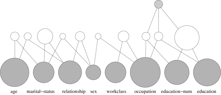
Figure 11: An informative conditional interaction graph illustrating the informative conditional interactions between the attributes with respect to the salary label in the ‘adult/census’ domain.

4 Handling Interactions in Supervised Learning

The machine learning community has long been aware of interactions, and many methods have been developed to deal with them. There are two problems that may arise from incorrect treatment of interactions: myopia is the consequence of assuming that interactions do not exist, even if they do exist; fragmentation is the consequence of acting as if interactions existed, when they are not significant. We will briefly survey several popular learning techniques in the light of the role they have with respect to interactions, and provide guidelines.

4.1 Myopia

Greedy feature selection and split selection heuristics are often based on various quantifications of 2-way interactions between the label $Y$ and an attribute $A$. The frequently used information gain heuristic in decision tree learning is a simple example of how interaction magnitude has been used for evaluating attribute importance. With more than a single attribute, information gain is no longer a reliable measure. First, with positive interactions, such as the exclusive or problem, information gain may underestimate the actual importance of attributes, since $I(A,B;Y)>I(A;Y)+I(B;Y)$. Second, in negative interactions, information gain will overestimate the importance of attributes, because some of the information is duplicated, as can be seen from $I(A,B;D)<I(A;D)+I(B;D)$.

These problems with positive interactions are known as myopia (Kononenko et al., 1997). Myopic feature selection evaluates an attribute’s importance independently of other attributes, and it is unable to appreciate their synergistic effect. The inability of myopic feature selection algorithms to appreciate interactions can be remedied with algorithms such as Relief (e.g. Kira and Rendell, 1992, Robnik-Šikonja and Kononenko, 2003), which increase the estimated quality of positively interacting attributes, and reduce the estimated worth of negatively interacting attributes.

Ignoring negative interactions may cause several problems in machine learning and statistics. We may end up with attributes providing the same information multiple times, hence biasing the predictions. For example, assume that the attribute $A$ is a predictor of the outcome $Y_{0}$, whereas the attribute $B$ predicts the outcome $Y_{1}$. If we duplicate $A$ into another attribute $A^{\prime}$ but retain a sole copy of $B$, naïve Bayesian classifier trained on $\{A,A^{\prime},B\}$ will be biased towards the outcome $Y_{0}$. Hence, negative interactions offer opportunity for eliminating redundant attributes, even if these attributes are informative on their own. An attribute $A^{\prime}$ would then be a conditionally irrelevant source of information about the label $Y$ given the attribute $A$ when $I(A^{\prime};Y|A)=0$, assuming that there are no other attributes positively interacting with the disposed attribute (Koller and Sahami, 1996). Indirectly, we could minimize the mutual information among the selected attributes, via eliminating $A^{\prime}$ if $I(A;A^{\prime})$ is large (Hall, 2000). Finally, attribute weighting, either explicit (by assigning weights to attributes) or implicit (such as fitting logistic regression models or support vector machines), helps remedy some examples of negative interactions. Not all examples of negative interactions are problematic, however, since conditional independence between two attributes given the label may result in a negative interaction information among all three.

Feature selection algorithms are not the only algorithms in machine learning that suffer from myopia. Most supervised discretization algorithms (e.g. Fayyad and Irani, 1993) are local and discretize one attribute at a time, determining the number of intervals with respect to the ability to predict the label. Such algorithms may underestimate the number of intervals for positively interacting attributes (Nguyen and Nguyen, 1998, Bay, 2001). For example, in a domain with two continuous attributes $X$ and $Y$, labelled with class $Z_{1}$ when $X>0,\,Y>0$ or $X<0,\,Y<0$, and with class $Z_{0}$ when $X>0,\,Y<0$ or $X<0,\,Y>0$ (the continuous version of the binary exclusive or problem), all univariate splits are uninformative. On the other hand, for negatively interacting attributes, the total number of intervals may be larger than necessary, causing fragmentation of the data. Hence, in case of positive and negative interactions, multivariate or global discretization algorithms may be preferred.

4.2 Fragmentation

To both take advantage of synergies and prevent redundancies, we may use a different set of more powerful methods. We may assume dependencies between attributes by employing dependence modelling (Kononenko, 1991, Friedman et al., 1997), create new attributes with structured induction methods (Shapiro, 1987, Pazzani, 1996, Zupan et al., 1999), or create new classes via class decomposition (Vilalta and Rish, 2003). The most frequently used methods, however, are the classification tree and rule induction algorithms. In fact, classification trees were originally designed also for detection of interactions among attributes in data: one of the first classification tree induction systems was named Automatic Interaction Detector (AID) (Morgan and Sonquist, 1963).

Classification trees are an incremental approach to modelling the joint probability distribution $P(Y|A,B,C)$. The information gain split selection heuristic (e.g. Quinlan, 1986) seeks the attribute $A$ with the highest mutual information with the label $Y$: $A=\arg\max_{X}{I(Y;X)}$. In the second step, we pursue the attribute $B$, which will maximize the mutual information with the label $Y$, but in the context of the attribute $A$ selected earlier: $B=\arg\max_{X}{I(Y;X|A)}$.

In case of negative interactions between $A$ and $B$, the classification tree learning method will correctly reduce $B$’s usefulness in the context of $A$, because $I(B;Y|A)<I(B;Y)$. If $A$ and $B$ interact positively, $B$ and $Y$ will have a larger amount of mutual information in the context of $A$ than otherwise, $I(B;Y|A)>I(B;Y)$. Classification trees enable proper treatment of positive interactions between the currently evaluated attribute and the other attributes already in the context. However, if the other positively interacting attribute has not been included in the tree already, then this positive 2-way interaction may be overlooked. To assure that positive interactions are not omitted, we may construct the classification tree with look-ahead (Norton, 1989, Ragavan and Rendell, 1993), or we may seek interactions directly (Pérez, 1997).

The classification tree learning approach does handle interactions, but it is not able to take all the advantage of mutually and conditionally independent attributes. Assuming dependence increases the complexity of the model because the dimensionality of the probability distributions estimated from the data is increased. A consequence of this is known as fragmentation (Vilalta et al., 1997), because the available mutual information between an attribute $B$ and the label $Y$ is not assessed on all the data, but merely on fragments of it. Fragmenting is harmful if the context $A$ is independent of the interaction between $B$ and $Y$. For example, if $I(B;Y)=I(B;Y|A)$, the information provided by $B$ about $Y$ should be gathered from all the instances, and not separately in each subgroup of instances with a particular value of the attribute $A$. This is especially important when the training data is scarce. Although we used classification trees as an example of a model that may induce fragmentation, other methods too are subject to fragmentation by assuming dependence unnecessarily.

Three approaches may be used to remedy fragmentation. One approach is based on ensembles: aggregations of simpler trees, each specializing in a specific interaction. For example, random forests (Breiman, 1999) aggregate the votes from a large number of small trees, where each tree can be imagined to be focusing on a single interaction. One can use hybrid methods that employ both classification trees and linear models that assume conditional independence, such as the naïve Bayesian classifier (Kononenko et al., 1988, Kohavi, 1996) or logistic regression (Abu-Hanna and de Keizer, 2003, Landwehr et al., 2003). Finally, feature construction algorithms may be employed in the context of classification tree induction (e.g. Pagallo and Haussler, 1990, Setiono and Liu, 1998).

5 Summary and Discussion

We have defined an interaction in a set of attributes to be the loss we incur by approximating the joint probability distribution of the attributes by only using marginal probability distributions. This notion is captured by McGill’s interaction information, a special case of which is mutual information. Interaction information has been independently rediscovered a number of times in a variety of fields, including machine learning, computational neuroscience, psychology and information and game theory. Interaction information can also be understood as a nonlinear generalization of correlation between any number of attributes. We can distinguish positive and negative interactions, depending on the sign of interaction information. Positive interactions indicate phenomena such as moderation, where one attribute affects the relationship of other attributes. On the other hand, negative interactions may suggest mediation, where one or more of the attributes in part convey the information already provided by other attributes.

The goal of interaction analysis is quantification of interactions and presentation of the interaction structure in the data in a comprehensible form to a human analyst. To this aim we have proposed a number of novel visualization methods that attempt to present interactions present in data, given some quantification of interactions. The interaction dendrogram is a compact summary of the attribute structure, identifying clusters of negatively interacting attributes, and connecting pairs of positively interacting attributes. The interaction graph identifies the most important interactions in detail. The information graph is a substitute for the Venn diagram and it illustrates the detailed structure of dependence in a small set of attributes. We show on numerous examples that the above quantifications usually confirm the intuitions.

There are two pitfalls that a good supervised learning procedure should avoid. The problem of myopia arises when a learning algorithm assumes that interactions do not exist, but they do. This results in the classifier bias. In myopic learning, negative interactions result in redundant models, while synergies between attributes are not taken advantage of. On the other hand, fragmentation is a consequence of assuming interactions when they do not exist or are not important enough. Fragmentation induces a learning procedure to gather statistics from less data than it could, causing unreliable estimates of evidence and the classifier variance. Fragmentation is also an issue for detecting interactions. To detect an interaction, we need to estimate the joint probability distribution of several variables. For this, a considerable amount of data is needed. For example, if one tries to do 3-way interaction analysis with only 100 instances, there will be a lot of noisy positive interactions, but few of them are significant. To solve this problem, the methods of statistical inference may be employed, for example hypothesis testing.

We are currently researching learning algorithms that are not sidetracked by or blind of interactions. Namely, pursuing interactions in data is complementary to pursuit of independence, but from the opposite direction. Starting with a simple model with no dependencies, we gradually build a complex one by successively introducing important interactions. One important problem in this context is the combinatorial explosion of the attribute combinations. However, one can employ heuristics, for example, higher-order interactions are unlikely in the absence of lower-order interactions among the same attributes. We are also developing methodology for investigating continuous attributes. Finally, in this text, we have made several assumptions, which are not always justified: attribute values are not always mutually independent, the instances are not always permutable. Relaxing these assumption is also an area for future research.

Acknowledgments

The authors wish to thank A. J. Bell and T. P. Minka for helpful comments and discussions, to S. Ravett Brown for providing the original McGill’s paper, to J. Dobša for drawing our attention to the issue of synonymy and polysemy, and to V. Batagelj for pointing us to Rajski’s work.

References

- Abu-Hanna and de Keizer (2003) A. Abu-Hanna and N. de Keizer. Integrating classification trees with local logistic regression in Intensive Care prognosis. Artificial Intelligence in Medicine, 29(1-2):5–23, Sep-Oct 2003.
- Amari (2001) S.-I. Amari. Information geometry on hierarchical decomposition of stochastic interactions. IEEE Trans. on Information Theory, 47(5):1701–1711, July 2001.
- Baron and Kenny (1986) R. M. Baron and D. A. Kenny. The moderator-mediator variable distinction in social psychological research: Conceptual, strategic and statistical considerations. Journal of Personality and Social Psychology, 51:1173–1182, 1986.
- Bartlett (1935) M. S. Bartlett. Contingency table interactions. Journal of the Royal Statistical Society, Suppl. 2:248–252, 1935.
- Bay (2001) S. D. Bay. Multivariate discretization for set mining. Knowledge and Information Systems, 3(4):491–512, 2001.
- Bell (2003) A. J. Bell. The co-information lattice. In ICA 2003, Nara, Japan, April 2003.
- Boes and Meyer (1999) J. L. Boes and C. R. Meyer. Multi-variate mutual information for registration. In C. Taylor and A. Colchester, editors, MICCAI 1999, volume 1679 of LNCS, pages 606–612. Springer-Verlag, 1999.
- Breiman (1999) L. Breiman. Random forests – random features. Technical Report 567, University of California, Statistics Department, Berkeley, 1999.
- Brenner et al. (2000) N. Brenner, S. P. Strong, R. Koberle, W. Bialek, and R. R. de Ruyter van Steveninck. Synergy in a neural code. Neural Computation, 12:1531 –1552, 2000.
- Cerf and Adami (1997) N. J. Cerf and C. Adami. Entropic Bell inequalities. Physical Review A, 55(5):3371 –3374, May 1997.
- Chechik et al. (2002) G. Chechik, A. Globerson, M. J. Anderson, E. D. Young, I. Nelken, and N. Tishby. Group redundancy measures reveal redundancy reduction in the auditory pathway. In T. G. Dietterich, S. Becker, and Z. Ghahramani, editors, NIPS 2002, pages 173–180, Cambridge, MA, 2002. MIT Press.
- Cheng et al. (2002) J. Cheng, R. Greiner, J. Kelly, D. A. Bell, and W. Liu. Learning Bayesian networks from data: an information-theory based approach. Artificial Intelligence Journal, 137:43–90, 2002.
- Cover and Thomas (1991) T. M. Cover and J. A. Thomas. Elements of Information Theory. Wiley Series in Telecommunications. John Wiley & Sons, 1991.
- Darroch (1974) J. N. Darroch. Multiplicative and additive interaction in contingency tables. Biometrika, 61(2):207–214, 1974.
- Fano (1961) R. M. Fano. The Transmission of Information: A Statistical Theory of Communication. MIT Press, Cambridge, Massachussets, March 1961.
- Fayyad and Irani (1993) U. M. Fayyad and K. B. Irani. Multi-interval discretization of continuous-valued attributes for classification learning. In IJCAI 1993, pages 1022–1027. AAAI Press, 1993.
- Freitas (2001) A. A. Freitas. Understanding the crucial role of attribute interaction in data mining. Artificial Intelligence Review, 16(3):177–199, November 2001.
- Friedman et al. (1997) N. Friedman, D. Geiger, and M. Goldszmidt. Bayesian network classifiers. Machine Learning, 29:131–163, 1997.
- Gat (1999) I. Gat. Statistical Analysis and Modeling of Brain Cells’ Activity. PhD thesis, Hebrew University, Jerusalem, Israel, 1999.
- Gediga and Düntsch (2003) G. Gediga and I. Düntsch. On model evaluation, indices of importance, and interaction values in rough set analysis. In S. K. Pal, L. Polkowski, and A. Skowron, editors, Rough-Neuro Computing: Techniques for computing with words. Physica Verlag, Heidelberg, 2003.
- Good (1965) I. J. Good. The Estimation of Probabilities: An Essay on Modern Bayesian Methods, volume 30 of Research Monograph. M.I.T. Press, Cambridge, Massachusetts, 1965.
- Grabisch and Roubens (1999) M. Grabisch and M. Roubens. An axiomatic approach to the concept of interaction among players in cooperative games. International Journal of Game Theory, 28(4):547–565, 1999.
- Hall (2000) M. A. Hall. Correlation-based feature selection for discrete and numeric class machine learning. In ICML 2000, Stanford University, CA, 2000. Morgan Kaufmann.
- Han (1980) T. S. Han. Multiple mutual informations and multiple interactions in frequency data. Information and Control, 46(1):26–45, July 1980.
- Hettich and Bay (1999) S. Hettich and S. D. Bay. The UCI KDD archive. Irvine, CA: University of California, Department of Information and Computer Science, 1999. URL http://kdd.ics.uci.edu.
- Jaccard (1908) P. Jaccard. Nouvelles recherches sur la distribution florale. Bulletin de la Societe Vaudoise de Sciences Naturelles, 44:223–270, 1908.
- Jakulin (2003) A. Jakulin. Attribute interactions in machine learning. Master’s thesis, University of Ljubljana, Faculty of Computer and Information Science, January 2003.
- Jakulin and Bratko (2003) A. Jakulin and I. Bratko. Analyzing attribute dependencies. In N. Lavrač, D. Gamberger, H. Blockeel, and L. Todorovski, editors, PKDD 2003, volume 2838 of LNAI, pages 229–240. Springer-Verlag, September 2003.
- Jakulin et al. (2003) A. Jakulin, I. Bratko, D. Smrke, J. Demšar, and B. Zupan. Attribute interactions in medical data analysis. In M. Dojat, E. Keravnou, and P. Barahona, editors, AIME 2003, volume 2780 of LNAI, pages 229–238. Springer-Verlag, October 2003.
- Kira and Rendell (1992) K. Kira and L. A. Rendell. A practical approach to feature selection. In D. Sleeman and P. Edwards, editors, ICML 1992, pages 249–256. Morgan Kaufmann, 1992.
- Kohavi (1996) R. Kohavi. Scaling up the accuracy of naive-Bayes classifiers: A decision-tree hybrid. In KDD 1996, pages 202–207, 1996.
- Koller and Sahami (1996) D. Koller and M. Sahami. Toward optimal feature selection. In L. Saitta, editor, ICML 1996, Bari, Italy, 1996. Morgan Kaufmann.
- Kononenko (1991) I. Kononenko. Semi-naive Bayesian classifier. In Y. Kodratoff, editor, EWSL 1991, volume 482 of LNAI. Springer Verlag, 1991.
- Kononenko et al. (1988) I. Kononenko, B. Cestnik, and I. Bratko. Assistant Professional User’s Guide. Jožef Stefan Institute, Ljubljana, Slovenia, 1988.
- Kononenko et al. (1997) I. Kononenko, E. Šimec, and Marko Robnik-Šikonja. Overcoming the myopia of inductive learning algorithms with RELIEFF. Applied Intelligence, 7(1):39–55, 1997.
- Kschischang et al. (2001) F. R. Kschischang, B. Frey, and H.-A. Loeliger. Factor graphs and the sum-product algorithm. IEEE Trans. on Information Theory, 47(2):498–519, 2001.
- Lancaster (1969) H. O. Lancaster. The Chi-Squared Distribution. J. Wiley & Sons, New York, 1969.
- Landwehr et al. (2003) N. Landwehr, M. Hall, and E. Frank. Logistic model trees. In N. Lavrač, D. Gamberger, H. Blockeel, and L. Todorovski, editors, ECML 2003, volume 2837 of LNAI, pages 241–252. Springer-Verlag, September 2003.
- López de Màntaras (1991) R. López de Màntaras. A distance based attribute selection measure for decision tree induction. Machine Learning, 6(1):81–92, 1991.
- MacKay (2003) D. MacKay. Information Theory, Inference, and Learning Algorithms. Cambridge University Press, October 2003.
- Manning and Schütze (1999) C. Manning and H. Schütze. Foundations of Statistical Natural Language Processing. MIT Press, Cambridge, MA, May 1999.
- Matsuda (2000) H. Matsuda. Physical nature of higher-order mutual information: Intrinsic correlations and frustration. Physical Review E, 62(3):3096–3102, September 2000.
- McGill (1954) W. J. McGill. Multivariate information transmission. Psychometrika, 19(2):97–116, 1954.
- Morgan and Sonquist (1963) J. N. Morgan and J. A. Sonquist. Problems in the analysis of survey data, and a proposal. Journal of the American Statistical Association, 58:415–435, 1963.
- Nguyen and Nguyen (1998) H. S. Nguyen and S. H. Nguyen. Discretization methods for data mining. In L. Polkowski and A. Skowron, editors, Rough Sets in Knowledge Discovery, pages 451–482. Physica-Verlag, Heidelberg, 1998.
- Norton (1989) S. W. Norton. Generating better decision trees. In IJCAI 1989, pages 800–805, 1989.
- Orlóci et al. (2002) L. Orlóci, M. Anand, and V. D. Pillar. Biodiversity analysis: issues, concepts, techniques. Community Ecology, 3(2):217–236, 2002.
- Pagallo and Haussler (1990) G. Pagallo and D. Haussler. Boolean feature discovery in empirical learning. Machine Learning, 5(1):71–99, March 1990.
- Paluš (1994) M. Paluš. Identifying and quantifying chaos by using information-theoretic functionals. In A. S. Weigend and N. A. Gerschenfeld, editors, Time Series Prediction: Forecasting the Future and Understanding the Past, NATO Advanced Research Workshop on Comparative Time Series Analysis, pages 387–413, Sante Fe, NM, May 1994. Addison-Wesley.
- Pazzani (1996) M. J. Pazzani. Searching for dependencies in Bayesian classifiers. In Learning from Data: AI and Statistics V. Springer-Verlag, 1996.
- Pearl (1988) J. Pearl. Probabilistic Reasoning in Intelligent Systems. Morgan Kaufmann, San Francisco, CA, USA, 1988.
- Pérez (1997) E. Pérez. Learning Despite Complex Attribute Interaction: An Approach Based on Relational Operators. PhD dissertation, University of Illinois at Urbana-Champaign, 1997.
- Quastler (1953) H. Quastler. The measure of specificity. In H. Quastler, editor, Information Theory in Biology. Univ. of Illinois Press, Urbana, 1953.
- Quinlan (1986) J. R. Quinlan. Induction of decision trees. Machine Learning, 1(1):81–106, 1986.
- Ragavan and Rendell (1993) H. Ragavan and L. A. Rendell. Lookahead feature construction for learning hard concepts. In ICML 1993, pages 252–259, 1993.
- Rajski (1961) C. Rajski. A metric space of discrete probability distributions. Information and Control, 4:373–377, 1961.
- Robnik-Šikonja and Kononenko (2003) M. Robnik-Šikonja and I. Kononenko. Theoretical and empirical analysis of ReliefF and RReliefF. Machine Learning, 53(1-2):23–69, 2003.
- Roy and Kastenbaum (1956) S. N. Roy and M. A. Kastenbaum. On the hypothesis of no ‘interaction’ in a multi-way contingency table. The Annals of Mathematical Statistics, 27:749–757, 1956.
- Rubinstein and Hastie (1997) Y. D. Rubinstein and T. Hastie. Discriminative vs informative learning. In SIGKDD 1997, pages 49–53. AAAI Press, August 1997.
- Setiono and Liu (1998) R. Setiono and H. Liu. Fragmentation problem and automated feature construction. In ICTAI 1998, pages 208–215, Taipei, Taiwan, November 1998. IEEE Computer Society.
- Shannon (1948) C. E. Shannon. A mathematical theory of communication. The Bell System Technical Journal, 27:379–423, 623–656, 1948.
- Shapiro (1987) A. D. Shapiro. Structured induction in expert systems. Turing Institute Press in association with Addison-Wesley Publishing Company, 1987.
- Sporns et al. (2000) O. Sporns, G. Tononi, and G. M. Edelman. Theoretical neuroanatomy: Relating anatomical and functional connectivity in graphs and cortical connection matrices. Cerebral Cortex, 10(2):127–141, February 2000.
- Studenỳ and Vejnarovà (1998) M. Studenỳ and J. Vejnarovà. The multiinformation function as a tool for measuring stochastic dependence. In M. I. Jordan, editor, Learning in Graphical Models, pages 261–297. Kluwer, 1998.
- Tsujishita (1995) T. Tsujishita. On triple mutual information. Advances in Applied Mathematics, 16:269–274, 1995.
- Vedral (2002) V. Vedral. The role of relative entropy in quantum information theory. Reviews of Modern Physics, 74, January 2002.
- Vilalta et al. (1997) R. Vilalta, G. Blix, and L. A. Rendell. Global data analysis and the fragmentation problem in decision tree induction. In ECML 1997, volume 1224 of LNAI, pages 312–326. Springer-Verlag, 1997.
- Vilalta and Rish (2003) R. Vilalta and I. Rish. A decomposition of classes via clustering to explain and improve naive Bayes. In N. Lavrač, D. Gamberger, H. Blockeel, and L. Todorovski, editors, ECML 2003, volume 2837 of LNAI, pages 444–455. Springer-Verlag, September 2003.
- Watanabe (1960) S. Watanabe. Information theoretical analysis of multivariate correlation. IBM Journal of Research and Development, 4:66–82, 1960.
- Wennekers and Ay (2003) T. Wennekers and N. Ay. Spatial and temporal stochastic interaction in neuronal assemblies. Theory in Biosciences, 122:5–18, 2003.
- Wong and Liu (1975) A. K. C. Wong and T. S. Liu. Typicality, diversity, and feature pattern of an ensemble. IEEE Trans. on Computers, C-24(2):158–181, February 1975.
- Yeung (1991) R. W. Yeung. A new outlook on Shannon’s information measures. IEEE Trans. on Information Theory, 37:466–474, May 1991.
- Yule (1907) G. U. Yule. On the theory of correlation for any number of variables, treated by a new system of notations. Proc. Roy. Soc., 79A:182–193, 1907.
- Zupan et al. (1999) B. Zupan, M. Bohanec, J. Demšar, and I. Bratko. Learning by discovering concept hierarchies. Artificial Intelligence, 109:211–242, 1999.