Manifold Learning with Geodesic Minimal Spanning Trees

Abstract

In the manifold learning problem one seeks to discover a smooth low dimensional surface, i.e., a manifold embedded in a higher dimensional linear vector space, based on a set of measured sample points on the surface. In this paper we consider the closely related problem of estimating the manifold’s intrinsic dimension and the intrinsic entropy of the sample points. Specifically, we view the sample points as realizations of an unknown multivariate density supported on an unknown smooth manifold. We present a novel geometrical probability approach, called the geodesic-minimal-spanning-tree (GMST), to obtaining asymptotically consistent estimates of the manifold dimension and the Rényi $\alpha$-entropy of the sample density on the manifold. The GMST approach is striking in its simplicity and does not require reconstructing the manifold or estimating the multivariate density of the samples. The GMST method simply constructs a minimal spanning tree (MST) sequence using a geodesic edge matrix and uses the overall lengths of the MSTs to simultaneously estimate manifold dimension and entropy. We illustrate the GMST approach for dimension and entropy estimation of a human face dataset.

Keywords: Nonlinear dimensionality reduction, geometrical probability, minimal spanning trees, intrinsic alpha-entropy, global manifold learning, conformal embeddings.

1 Introduction

Consider a class of natural occurring signals, e.g., recorded speech, audio, images, or videos. Such signals typically have high extrinsic dimension, e.g., as characterized by the number of pixels in an image or the number of time samples in an audio waveform. However, most natural signals have smooth and regular structure, e.g. piecewise smoothness, that permits substantial dimension reduction with little or no loss of content information. For support of this fact one needs only consider the success of image, video and audio compression algorithms, e.g. MP3, JPEG and MPEG, or the widespread use of efficient computational geometry methods for rendering smooth three dimensional shapes.

A useful representation of a regular signal class is to model it as a set of vectors which are constrained to a smooth low dimensional manifold embedded in a high dimensional vector space. This manifold may in some cases be a linear, i.e., Euclidean, subspace but in general it is a non-linear curved surface. A problem of substantial recent interest in machine learning, computer vision, signal processing and statistics [34, 14, 27, 16, 26, 35] is the determination of the so-called intrinsic dimension of the manifold and the reconstruction of the manifold from a set of samples from the signal class. This problem falls in the area of manifold learning which is concerned with discovering low dimensional structure in high dimensional data.

When the samples are drawn from a large population of signals one can interpret them as realizations from a multivariate distribution supported on the manifold. As this distribution is singular in the higher dimensional embedding space it has zero entropy as defined by the standard Lebesgue integral over the embedding space. However, when defined as a Lebesgue integral restricted to the lower dimensional manifold the entropy can be finite. This finite “intrinsic” entropy can be useful for for exploring data compression over the manifold or, as suggested in [21], clustering of multiple sub-populations on the manifold. The question that we address in this paper is: how to simultaneously estimate the intrinsic dimension and intrinsic entropy on the manifold given a set of random sample points? We present a novel geometrical probability approach to this question which is based on entropic graph methods developed by us and reported in publications [23, 21, 20].

Techniques for manifold learning can be classified into three categories: linear methods, local methods, and global methods. Linear methods include principal components analysis (PCA) [25] and multidimensional scaling (MDS) [12]. They are based on analyzing eigenstructure of empirical covariance matrices, and can be reliably applied only when the manifold is a linear subspace. Local methods include linear local imbedding (LLE) [32], locally linear projections (LLP) [24], Laplacian eigenmaps [4], and Hessian eigenmaps [16]. They are based on local approximation of the geometry of the manifold, and are computationally simple to implement. Global approaches include ISOMAP [34] and C-ISOMAP [15]. They preserve the manifold geometry at all scales, and have better stability than local methods.

We propose a geodesic-minimal-spanning-tree (GMST) method for manifold learning that is implemented as follows. First a complete geodesic graph between all pairs of data samples is constructed, e.g. using ISOMAP or C-ISOMAP. Then a minimal spanning graph, the GMST, is obtained by pruning the complete geodesic graph down to a subgraph that still connects all points but has minimum total geodesic length. The intrinsic dimension and intrinsic $\alpha$-entropy is then estimated from the GMST length functional using a simple linear least squares (LLS) and method of moments (MOM) procedure.

The GMST method falls in the category of global approaches to manifold learning but it differs significantly from the aforementioned methods. First, it has a different scope. Indeed, unlike ISOMAP and C-ISOMAP, the GMST method provides a statistically consistent estimate of the intrinsic entropy in addition to the intrinsic dimension of the manifold. To the best of our knowledge no other such technique has been proposed for learning manifold dimension. Second, unlike local methods that work on chunks of data in local neighborhoods, GMST works on chunks of resampled data over the global data set. Third, for $N$ samples the GMST method has $O(N\log N)$ computational complexity as compared with the $O(N^{3})$ complexity of an MDS ISOMAP reconstruction. Fourth, the GMST method is simple and elegant: it estimates intrinsic entropy and dimension by detecting the rate of increase of a GMST as a function of the number of its resampled vertices.

The aims of this paper are limited to introducing GMST as a novel method for estimating manifold dimension and entropy of the samples. As in work of others on dimension estimation [26, 8] we do not here consider the issue of reconstruction of the complete manifold. Similarly to these authors, we believe that dimension estimation and entropy estimation for non-linear data are of interest in their own right. We also do not consider the effect of additive noise or outliers on the performance of GMST. Finally, the consistency results of GMST reported here are limited to domain manifolds defined by some smooth unknown mapping. The extension of GMST methodology to general target manifolds, e.g. those defined by implicit level set embeddings [29, 28], is a worthwhile topic for future investigation.

What follows is a brief outline of the paper. We review some necessary background on the mathematics of domain manifolds in Sec. 2. In Sec. 3 we review the asymptotic theory of entropic graphs and obtain several new results required for their extension to embedded manifolds. In Sec. 4 we define the general GMST algorithm. Finally in Sec. 5 we illustrate the GMST approach to estimating intrinsic dimension and entropy of a human face dataset.

2 Background

2.1 A 3D Example

To illustrate ideas consider a 2D surface embedded in 3D Euclidean space, called the embedding space. Let $\{\mbox{\boldmath$x$}_{1},\mbox{\boldmath$x$}_{2},\ldots\}\subset U\subseteq\mathbb{R}^{2}$ be a set of points (samples) in a subset $U$ of the plane. Naturally, the shortest path between any pair $(\mbox{\boldmath$x$}_{i},\mbox{\boldmath$x$}_{j})$ of these points is given by the straight line in $\mathbb{R}^{2}$ connecting them, with corresponding distance given by its Euclidean ($L_{2}$) length, $|\mbox{\boldmath$x$}_{i}-\mbox{\boldmath$x$}_{j}|_{2}$. Now let $U$ be used as a parameterization space to describe a curved surface in $\mathbb{R}^{3}$ via a mapping $\varphi:U\rightarrow\mathbb{R}^{3}$. Surfaces $\mathcal{M}=\varphi(U)$ defined in this explicit manner are called domain manifolds and they inherit the topological dimension, equal to 2 in this case, of the parameterization space. When $\varphi$ is non-linear the shortest path on $\mathcal{M}$ between points $\mbox{\boldmath$y$}_{i}=\varphi(\mbox{\boldmath$x$}_{i})$ and $\mbox{\boldmath$y$}_{j}=\varphi(\mbox{\boldmath$x$}_{j})$ is a curve on the surface called the geodesic curve. In this paper we will primarily consider domain manifolds defined by conformal mappings $\varphi$. Such conformal embeddings have the property that the length of paths on the surface are identical to lengths of paths in the parameterization space, possibly up to a smoothly varying local scale factor. This property guarantees that, regardless of how the mapping $\varphi$ “deforms” $U$ onto $\mathcal{M}$, the geodesic distances in $\mathcal{M}$ are closely related to the Euclidean distances in $U$. When this smooth surface representation holds there exist algorithms, e.g. ISOMAP and C-ISOMAP [34, 15], which can be used to estimate the Euclidean distances between points in $U$ from estimates of the geodesic distances between points in $\mathcal{M}$. If a certain type of minimal spanning graph is constructed using these estimates well established results in geometrical probability [36, 21] allow us to develop simple estimates of both entropy and dimension of the points distributed on the surface.

2.2 Differential Geometry Setting

In the following, we recall some facts from differential geometry needed to formalize and generalize the ideas just described. We will consider smooth manifolds embedded in $\mathbb{R}^{d}$. For the general theory we refer the reader to any standard book in differential geometry (for example, [9], [10], [7]). An $m$-dimensional smooth manifold $\mathcal{M}\subseteq\mathbb{R}^{d}$ is a set such that each of its points has a neighborhood that can be parameterized by an open set of $\mathbb{R}^{m}$ through a local change of coordinates. Intuitively, this means that although $\mathcal{M}$ is a (hyper) surface in $\mathbb{R}^{d}$, it can be locally identified with $\mathbb{R}^{m}$.

Let $\varphi:\Omega\mapsto\mathcal{M}$ be a mapping between two manifolds, $\Omega,\mathcal{M}$. Let $\gamma$ be a curve in $\Omega$. The tangent map $\mathrm{d}{\varphi}_{\mbox{\boldmath$x$}}$ assigns each tangent vector $v$ to $\Omega$ at point $x$ the tangent vector $\mathrm{d}{\varphi}_{\mbox{\boldmath$x$}}\mbox{\boldmath$v$}$ to $\mathcal{M}$ at point $\varphi(\mbox{\boldmath$x$})$, such that, if $v$ is the initial velocity of $\gamma$ in $\Omega$, then $\mathrm{d}{\varphi}_{\mbox{\boldmath$x$}}\mbox{\boldmath$v$}$ is the initial velocity of the curve $\varphi(\gamma)$ in $\mathcal{M}$. For example, if $\mbox{\boldmath$x$}\in U\subseteq\Omega\subseteq\mathbb{R}^{m}$, with $U$ an open set of $\mathbb{R}^{m}$, then $\mathrm{d}{\varphi}_{\mbox{\boldmath$x$}}\mbox{\boldmath$v$}=\mathsfsl{J}_{\varphi}(\mbox{\boldmath$x$})\,\mbox{\boldmath$v$}$, where $\mathsfsl{J}_{\varphi}=[\partial\varphi_{i}/\partial x_{j}]$, $i=1,\ldots,d$, $j=1,\ldots,m$, is the Jacobian matrix associated with $\varphi$ at point $\mbox{\boldmath$x$}\in\Omega$.

The length of a smooth curve $\Gamma:[0,1]\mapsto\mathcal{M}$ is defined as $\ell(\Gamma)=\int_{0}^{1}|\dot{\Gamma}(t)|\mathrm{d}{t}$. The geodesic distance between points $\mbox{\boldmath$y$}_{0},\mbox{\boldmath$y$}_{1}\in\mathcal{M}$ is the length of the shortest (piecewise) smooth curve between the two points:

$$d_{\mathcal{M}}(\mbox{\boldmath$y$}_{0},\mbox{\boldmath$y$}_{1})=\inf_{\Gamma}\{\ell(\Gamma):\Gamma(0)=\mbox{\boldmath$y$}_{0},\Gamma(1)=\mbox{\boldmath$y$}_{1}\}\ .$$

We can now define the following types of embeddings.

Definition 1

$\varphi:\Omega\mapsto\mathcal{M}$ is called a conformal mapping if $\varphi$ is a diffeomorphism (i.e., $\varphi$ is differentiable, bijective with differentiable inverse $\varphi^{-1}$) and, at each point $\mbox{\boldmath$x$}\in\Omega$, $\varphi$ preserves the angles between tangent vectors, i.e.,

$$\left(\mathrm{d}{\varphi}_{\mbox{\boldmath$x$}}\mbox{\boldmath$v$}\right)^{T}\left(\mathrm{d}{\varphi}_{\mbox{\boldmath$x$}}\mbox{\boldmath$w$}\right)=c(\mbox{\boldmath$x$})\,\mbox{\boldmath$v$}^{T}\mbox{\boldmath$w$}\ ,$$ (1)

for all vectors $v$ and $w$ that are tangent to $\Omega$ at $x$, and $c(\mbox{\boldmath$x$})>0$ is a scaling factor that varies smoothly with $x$. If for all $\mbox{\boldmath$x$}\in\Omega$, $c(\mbox{\boldmath$x$})=1$, then $\varphi$ is said to be a (global) isometry. In this case the length of tangent vectors is also preserved in addition to the angles between them.

It is easy to check that if there is an open set $U\subseteq\Omega\subseteq\mathbb{R}^{m}$, then the diffeomorphism $\varphi$ is a conformal mapping iff $\mathsfsl{J}_{\varphi}(\mbox{\boldmath$x$})^{T}\mathsfsl{J}_{\varphi}(\mbox{\boldmath$x$})=c(\mbox{\boldmath$x$})\,\mathsfsl{I}_{m}$, where $\mathsfsl{I}_{m}$ is the $m\times m$ identity matrix. In this case, the geodesic distance in $\mathcal{M}$ can be computed as follows. Any smooth curve $\Gamma:[0,1]\mapsto\mathcal{M}$ can be represented as $\Gamma(t)=\varphi(\gamma(t))$, where $\gamma:[0,1]\mapsto\Omega$ is a smooth curve in $\mathbb{R}^{m}$. Then, the length $\ell(\Gamma)$ of the curve $\Gamma$ is given by

$$\ell(\Gamma) = \int_{0}^{1}\left|\frac{\mathrm{d}{}}{\mathrm{d}{t}}\varphi(\gamma(t))\right|\mathrm{d}{t}$$

$$= \int_{0}^{1}|\mathsfsl{J}_{\varphi}(\gamma(t))\,\dot{\gamma}(t)|\,\mathrm{d}{t}=\int_{0}^{1}\sqrt{c(\gamma(t))}\,|\dot{\gamma}(t)|\,\mathrm{d}{t}\ .$$

As in $\mathbb{R}^{m}$ the shortest path between any two points is given by the straight line that connects them, $\gamma(t)=\mbox{\boldmath$x$}_{0}+t(\mbox{\boldmath$x$}_{1}-\mbox{\boldmath$x$}_{0})$ minimizes $\int_{0}^{1}|\dot{\gamma}(t)|\,\mathrm{d}{t}$, over all smooth curves with start and end points at $\mbox{\boldmath$x$}_{0}$ and $\mbox{\boldmath$x$}_{1}$, respectively. So, if $c(\mbox{\boldmath$x$})=c$, for all $x\in\Omega$, the geodesic distance between $\mbox{\boldmath$y$}_{0}=\varphi(\mbox{\boldmath$x$}_{0})$ and $\mbox{\boldmath$y$}_{1}=\varphi(\mbox{\boldmath$x$}_{1})$ is

$$d_{\mathcal{M}}(\varphi(\mbox{\boldmath$x$}_{0}),\varphi(\mbox{\boldmath$x$}_{1}))=c|\mbox{\boldmath$x$}_{0}-\mbox{\boldmath$x$}_{1}|_{2}\ .$$ (2)

When $c=1$, i.e., $\varphi$ is an isometry, the geodesic distance in $\mathcal{M}$ and the Euclidean distance in the parameterization space $\mathbb{R}^{m}$ are the same. If $c>1$ ($c<1$) there is a global expansion (contraction) in the distances between points.

It is evident from the above discussion that geodesic distances carry strong information about a non-linear domain manifold such as $\mathcal{M}$. However, their computation requires the knowledge of the analytical form of $\mathcal{M}$ via $\varphi$ and its Jacobian. In the manifold learning scenario considered in this paper this analytical form is assumed unknown and, instead, we are given a finite set of data points lying on the smooth $m$-dimensional manifold $\mathcal{M}$, with $m$ also considered unknown. In order to reconstruct a domain manifold along with its parameterization we need to estimate the geodesic distances between pairs of data points in $\mathcal{M}$ and the respective Euclidean distances betweem pre-images of these data points in the parameterization space $U$.

When $\mathcal{M}$ is an isometric embedding the ISOMAP algorithm [34] obtains such a reconstruction from a finite set of samples through estimation of the pairwise geodesic distances. This estimate is computed from a Euclidean graph $G$ connecting all local neighborhoods of data points in $\mathcal{M}$. Specifically, ISOMAP proceeds as follows. Two methods, called the $\epsilon$-rule and the $k$-rule [34], have been proposed for contructing $G$. The first method connects each point to all points within some fixed radius $\epsilon$ and the other connects each point to all its $k$-nearest neighbors. The graph $G$ defining the connectivity of these local neighborhoods is then used to approximate the geodesic distance between any pair of points as the shortest path through $G$ that connects them. This results in an edge matrix whose $(i,j)$ entry is the geodesic distance estimate for the $(i,j)$-th pair of points. Finally, ISOMAP obtains a smooth reconstruction of the manifold by applying the classical Multidimensional Scaling (MDS) method [12] to the edge matrix.

Step 1.

Determine a Euclidean neighborhood graph $G$ of the observed data $\mathcal{Y}_{n}$ according to the $\epsilon$-rule or the $k$-rule as defined in ISOMAP [5].

Step 2.

For isometric embeddings compute the edge matrix ${\mathcal{E}}$ of the ISOMAP graph [34] and for conformal imbeddings compute the edge matrix ${\mathcal{E}}$ of the C-ISOMAP graph [15]. The $(i,j)$ entry of this symmetric matrix is the sum of the lengths of the edges in $G$ along the shortest path between the pair of vertices $(\mbox{\boldmath$Y$}_{i},\mbox{\boldmath$Y$}_{j})$ where the edge lengths between neighboring points $\mbox{\boldmath$Y$}_{1}$, $\mbox{\boldmath$Y$}_{2}$ in $G$ are defined as Euclidean distance $|\mbox{\boldmath$Y$}_{1}$-$\mbox{\boldmath$Y$}_{2}|$ in the case of ISOMAP or $|\mbox{\boldmath$Y$}_{1}$-$\mbox{\boldmath$Y$}_{2}|/\sqrt{M(1)M(2)}$ in the case of C-ISOMAP where $M(i)$ is the mean distance of $\mbox{\boldmath$Y$}_{i}$ to its immediate nearest neighbors.

Table 1: First two steps of the ISOMAP/C-ISOMAP algorithms to reconstruct Euclidean distances between ${\mathcal{X}}_{n}$ on the embedding parameterization space from points ${\mathcal{Y}}_{n}$ over the embedded manifold

Steps one and two of ISOMAP are motivated by the fact that locally any smooth manifold is approximately “flat” and, so, the distances between neighboring points are well approximated by their Euclidean distances. For faraway points, the geodesic distance is estimated by summing the sequence of such local approximations over the shortest path through the graph $G$. In [5] it was proved that, when the data are random samples from a continuous distribution on the manifold $\mathcal{M}$, the first two steps of ISOMAP recover the true geodesic distances with high probability if the data points form a sufficiently “dense” sampling of $\mathcal{M}$ and if $\mathcal{M}$ is free of “holes.” When $\mathcal{M}$ is a global isometric embedding in $\mathbb{R}^{d}$, the estimated geodesic distances are also an estimate of distances in $\mathbb{R}^{m}$ and the ISOMAP succeeds in its task of manifold reconstruction. For other types of embeddings, there is no guarantee that the ISOMAP will recover the correct parameterization. In [14], a variant of this algorithm, called C-ISOMAP, was proposed to deal with the more general class of conformal embeddings.

With regards to estimation of the intrinsic dimension $m$ several methods have been proposed [25]. Most of these methods are based on linear projection techniques: a linear map is explicitly constructed and dimension is estimated by applying Principal Component Analysis (PCA), factor analysis, or MDS to analyze the eigenstructure of the data. These methods rely on the assumption that only a small number of the eigenvalues of the (processed) data covariance will be significant. Linear methods tend to overestimate $m$ as they don’t account for non-linearities in the data. Both nonlinear PCA [27] methods and the ISOMAP circumvent this problem but they still rely on unreliable and costly eigenstructure estimates. Other methods have been proposed based on local geometric techniques, e.g., estimation of local neighborhoods [35] or fractal dimension [8], and estimating packing numbers [26] of the manifold.

3 Entropic Graph Estimators on Embedded Manifolds

Let ${\mathcal{Y}}_{n}=\mbox{\boldmath$Y$}_{1},\ldots,\mbox{\boldmath$Y$}_{n}$ be $n$ independent identically distributed (i.i.d.) random vectors in $[0,1]^{d}$, with multivariate Lebesgue density $f$, which we will also call random vertices. Define the edge matrix ${\mathcal{E}}$ as the $n\times n$ matrix of edge lengths (w.r.t. a specified metric) between pairs of vertices. A spanning graph $T$ over ${\mathcal{Y}}_{n}$ is defined as the pair $\{V,E\}$ where $V={\mathcal{Y}}_{n}$ and $E$ is a subset of edges from ${\mathcal{E}}$ which connect the vertices $V$. When ${\mathcal{E}}$ is computed from pairwise Euclidean distances $T$ is called a Euclidean spanning graph.

It has long been known [3] that, when suitably normalized, the sum of the edge weights of certain minimal Euclidean spanning graphs $T$ over ${\mathcal{Y}}_{n}$ converges almost surely (a.s.) to the limit $\beta_{d}\int_{\mathbb{R}^{d}}f^{\alpha}(\mbox{\boldmath$y$})d\mbox{\boldmath$y$}$ where where the integral is interpreted in the sense of Lebesgue, $\alpha\in(0,1)$ and $\beta_{d}>0$. This a.s. limit is the integral factor $\int f^{\alpha}$ in what we will call the extrinsic Rényi $\alpha$-entropy of the multivariate Lebesgue density $f$:

$$H_{\alpha}^{\mathbb{R}^{d}}(f)=\frac{1}{1-\alpha}\log\int_{\mathbb{R}^{d}}f^{\alpha}(\mbox{\boldmath$y$})d\mbox{\boldmath$y$}\ .$$ (3)

In the limit, when $\alpha\to 1$ we obtain the usual Shannon entropy, $-\int_{\mathbb{R}^{d}}f(\mbox{\boldmath$y$})\log f(\mbox{\boldmath$y$})\mathrm{d}\mbox{\boldmath$y$}$. Graph constructions that converge to the integral in the limit (3) were called continuous quasi-additive (Euclidean) graphs in [36] and entropic (Euclidean) graphs in [21]. See the monographs by Steele [33] and Yukich [36] for an excellent introduction to the theory of such random Euclidean graphs.

The $\alpha$-entropy has proved to be an important quantity in signal processing, where its applications range from vector quantization [18, 31] to pattern matching [22] and image registration [21, 19]. The $\alpha$-entropy parameterizes the Chernoff exponent governing the minimum probability of error [11] making it an important quantity in detection and classification problems. Like the Shannon entropy, the $\alpha$-entropy also has an operational characterization in terms of source coding rates. In [13] it was shown that the $\alpha$-entropy of a source determines the achievable block-code rates in the sense that the probability of block decoding error converges to zero at an exponential rate with rate constant $H_{\alpha}^{\mathbb{R}^{d}}(f)$.

3.1 Beardwood-Halton-Hammersley Theorem in $\mathbb{R}^{d}$

A remarkable result in geometrical probability was established by Beardwood, Halton and Hammersley almost half a century ago [3]. Let $\mathcal{Y}_{n}=\{\mbox{\boldmath$Y$}_{1},\ldots,\mbox{\boldmath$Y$}_{n}\}$ be a set of points in $\mathbb{R}^{d}$. A minimal Euclidean graph spanning ${\mathcal{Y}}_{n}$ is defined as the graph spanning ${\mathcal{Y}}_{n}$ having minimal overall length

$$L^{\mathbb{R}^{d}}_{\gamma}({\mathcal{Y}}_{n})=\min_{T\in\mathcal{T}}\sum_{e\in T}|e|^{\gamma}\ .$$ (4)

Here the sum is over all edges $e$ in the graph $T$, $|e|$ is the Euclidean length of $e$, and $\gamma\in(0,d)$ is called the edge exponent or power-weighting constant. For example when $\mathcal{T}$ is the set of spanning trees over $\mathcal{Y}_{n}$ one obtains the MST. A minimal Euclidean graph is continuous quasi-additive when it satisfies several technical conditions specified in [36] (also see [23]). Continuous quasi-additive Euclidean graphs include: the minimal spanning tree (MST), the $k$-nearest neighbors graph ($k$-NNG), the minimal matching graph (MMG), the traveling salesman problem (TSP), and their power-weighted variants. While all of the results in this paper apply to this larger class of minimal graphs we specialize to the MST for concreteness.

Beardwood-Halton-Hammersley (BHH) Theorem [33, 36]: Let ${\mathcal{Y}}_{n}$ be an i.i.d. set of random variables taking values in $\mathbb{R}^{d}$ having common probability distribution $P$. Let this distribution have the decomposition $P=F+Q$ where $F$ is the Lebesgue continuous component and $Q$ is the singular component. The Lebesgue continuous component has a Lebesgue density (no delta functions) which is denoted $f(x)$, $x\in\mathbb{R}^{d}$. Let $L^{\mathbb{R}^{d}}_{\gamma}({\mathcal{Y}}_{n})$ be the length of the MST spanning ${\mathcal{Y}}_{n}$ and assume that $d\geq 2$ and $0<\gamma<d$. Then

$$L^{\mathbb{R}^{d}}_{\gamma}(\mathcal{Y}_{n})/n^{\alpha}\rightarrow\beta_{d}\int_{\mathbb{R}^{d}}f^{\alpha}(\mbox{\boldmath$y$})d\mbox{\boldmath$y$}\;\;\;\ (a.s.),$$ (5)

where $\alpha=(d-\gamma)/d$ and $\beta_{d}$ is a constant not depending on the distribution $P$. Furthermore, the mean length $E[L^{\mathbb{R}^{d}}_{\gamma}({\mathcal{Y}}_{n})]/n^{\alpha}$ converges to the same limit.

The limit on the right side of (5) in the BHH theorem is zero when the distribution $P$ has no Lebesgue continuous component, i.e., when $F\equiv 0$. On the other hand, when $P$ has no singular component, i.e., $Q\equiv 0$, a consequence of the BHH Theorem is that

$$\hat{H}_{\alpha}^{\mathbb{R}^{d}}({\mathcal{Y}}_{n})\;\mbox{$\stackrel{{\scriptstyle\mbox{\rm def}}}{{=}}$}\;\frac{d}{\gamma}\left[\log\frac{L^{\mathbb{R}^{d}}_{\gamma}(\mathcal{Y}_{n})}{n^{(d-\gamma)/d}}-\log\beta_{d}\right]$$ (6)

is an asymptotically unbiased and strongly consistent estimator of the extrinsic $\alpha$-entropy $H_{\alpha}^{\mathbb{R}^{d}}(f)$ defined in (3).

3.2 Generalization of BHH Thm. to Embedded Manifolds

If the vertices ${\mathcal{Y}}_{n}=\{\mbox{\boldmath$Y$}_{1},\ldots,\mbox{\boldmath$Y$}_{n}\}$ are constrained to lie on a smooth $m$-dimensional manifold $\mathcal{M}\subset[0,1]^{d}$, the distribution of $\mbox{\boldmath$Y$}_{i}$ is singular with respect to Lebesgue measure, $F\equiv 0$, and, as previously mentioned, the limit (5) in the BHH Theorem is zero. However, as shown below, if $\mathcal{M}$ is defined by an isometric embedding from the parameterization space $\mathbb{R}^{m}$, if $\mbox{\boldmath$Y$}_{i}$ has a continuous density $f$ on $\mathcal{M}$, and if ISOMAP is used to approximate the geodesic edge matrix, then the length of an MST constructed from the geodesic edge matrix can be made to converge, after suitable normalization and transformation, to the intrinsic $\alpha$-entropy $H_{\alpha}^{\mathcal{M}}(f)$ on $\mathcal{M}$ defined by

$$H_{\alpha}^{\mathcal{M}}(f)=\frac{m}{\gamma}\log\int_{\mathcal{M}}f^{\alpha}(\mbox{\boldmath$y$})\mu_{\mathcal{M}}(d\mbox{\boldmath$y$}),$$ (7)

where $\mu_{\mathcal{M}}(d\mbox{\boldmath$y$})$ denotes the differential volume element over $\mathcal{M}$.

More generally, assume that $\mathcal{M}$ is embedded in $[0,1]^{d}$ through the diffeomorphism $\varphi$. As $\mbox{\boldmath$X$}_{i}=\varphi^{-1}(\mbox{\boldmath$Y$}_{i})$ lives in $\mathbb{R}^{m}$, let $T$ be the Euclidean minimal graph spanning ${\mathcal{X}}_{n}$ and having length function $L^{\mathbb{R}^{m}}_{\gamma}\left(\mathcal{X}_{n}\right)=L^{\mathbb{R}^{m}}_{\gamma}\left(\varphi^{-1}(\mathcal{Y}_{n})\right)$ according to definition (4). We have the following extension of the BHH Theorem.

Theorem 1

Let $\mathcal{M}$ be a smooth compact $m$-dimensional manifold embedded in $[0,1]^{d}$ through the diffeomorphism $\varphi:\mathbb{R}^{m}\mapsto\mathcal{M}$. Assume $2\leq m\leq d$ and $0<\gamma<m$. Suppose that $\mbox{\boldmath$Y$}_{1},\mbox{\boldmath$Y$}_{2},\ldots$ are i.i.d. random vectors on $\mathcal{M}$ having common density $f$ with respect to Lebesgue measure $\mu_{\mathcal{M}}$ on $\mathcal{M}$. Then, the length functional $L^{\mathbb{R}^{m}}_{\gamma}(\varphi^{-1}({\mathcal{Y}}_{n}))$ of the MST spanning $\varphi^{-1}({\mathcal{Y}}_{n})$ satisfies

$$\lim_{n\to\infty}L^{\mathbb{R}^{m}}_{\gamma}(\varphi^{-1}({\mathcal{Y}}_{n}))/n^{(d^{{}^{\prime}}-\gamma)/d^{{}^{\prime}}}\to$$ (8)

$$\left\{\begin{array}[]{cc}\infty,&d^{{}^{\prime}}<m\\ \\ \beta_{m}\int_{\mathcal{M}}\left[\det\left(\mathsfsl{J}_{\varphi}^{T}\mathsfsl{J}_{\varphi}\right)\right]^{\frac{\alpha-1}{2}}f^{\alpha}(\mbox{\boldmath$y$})\,\mu_{\mathcal{M}}(d\mbox{\boldmath$y$}),&d^{{}^{\prime}}=m\\ \\ 0,&d^{{}^{\prime}}>m\end{array}\right.$$ (14)

(a.s.) where $\alpha=(m-\gamma)/m$. Furthermore, the mean $E[L^{\mathbb{R}^{m}}_{\gamma}(\varphi^{-1}({\mathcal{Y}}_{n}))]/n^{(d^{{}^{\prime}}-\gamma)/d^{{}^{\prime}}}$ converges to the same limit.

This theorem is a simple consequence of the relation (5) in the BHH Theorem and properties of integrals over manifolds.

Proof of Thm. 1: By the BHH Theorem, with probability one

$$L^{\mathbb{R}^{m}}_{\gamma}({\mathcal{X}}_{n})=n^{(m-\gamma)/m}\beta_{m}\;\int_{\mathbb{R}^{m}}f^{\alpha}_{X}(\mbox{\boldmath$x$})\,d\mbox{\boldmath$x$}+o(n^{(m-\gamma)/m}),$$ (15)

where $f_{X}$ is the density of $\mbox{\boldmath$X$}_{i}=\varphi^{-1}(\mbox{\boldmath$Y$}_{i})$. Therefore the limits claimed in (8) for $d^{{}^{\prime}}<m$ and $d^{{}^{\prime}}>m$ are obvious. For $d^{{}^{\prime}}=m$ the relation (15) implies

$$\lim_{n\rightarrow\infty}L^{\mathbb{R}^{m}}_{\gamma}({\mathcal{X}}_{n})/n^{(m-\gamma)/m}=\beta_{m}\;\int_{\mathbb{R}^{m}}f^{\alpha}_{X}(\mbox{\boldmath$x$})\,d\mbox{\boldmath$x$},$$ (16)

and it remains to show that this limit is identical to the limit asserted in (8).

For an integrable function $F$ defined on a domain manifold $\mathcal{M}$ defined by the diffeomorphism $\varphi:\mathbb{R}^{m}\mapsto\mathcal{M}$, the integral of $F$ over $\mathcal{M}$ satisfies the relation [10]:

$$\int_{\mathcal{M}}F(\mbox{\boldmath$y$})\,\mu_{\mathcal{M}}(d\mbox{\boldmath$y$})=\int_{\mathbb{R}^{m}}F(\varphi(\mbox{\boldmath$x$}))\,g(\mbox{\boldmath$x$})\,d\mbox{\boldmath$x$}\ ,$$ (17)

where $g(\mbox{\boldmath$x$})=\sqrt{\det\left(\mathsfsl{J}_{\varphi}^{T}\mathsfsl{J}_{\varphi}\right)}$. Specializing $F$ to the indicator function of a small volume centered at a point $y$ (17) implies the following relation between volume elements in $\mathcal{M}$ and $\mathbb{R}^{m}$: $\mu_{\mathcal{M}}(d\mbox{\boldmath$y$})=g(\mbox{\boldmath$x$})\,d\mbox{\boldmath$x$}.$ Furthermore, specializing to $F(\mbox{\boldmath$y$})=f(\mbox{\boldmath$y$})$ it is clear from (17) that $f_{X}(\mbox{\boldmath$x$})=f(\varphi(\mbox{\boldmath$x$}))g(\mbox{\boldmath$x$})$. Therefore

$$\int_{\mathbb{R}^{m}}f_{X}^{\alpha}(\mbox{\boldmath$x$})d\mbox{\boldmath$x$} = \int_{\mathbb{R}^{m}}(f(\varphi(\mbox{\boldmath$x$}))g(\mbox{\boldmath$x$}))^{\alpha}d\mbox{\boldmath$x$}$$

$$= \int_{\mathbb{R}^{m}}f^{\alpha}(\varphi(\mbox{\boldmath$x$}))g^{\alpha-1}(\mbox{\boldmath$x$}))\;g(\mbox{\boldmath$x$})d\mbox{\boldmath$x$},$$

which, after the change of variable $\mbox{\boldmath$x$}\mapsto\varphi(\mbox{\boldmath$x$})$, is equivalent to the integral in the limit (8). $\Box$

Our goal is to learn the entropy of non-linear data on a domain manifold together with its intrinsic dimension, given only the data set $\mathcal{Y}_{n}$ of $n$ samples in the embedding space $\mathbb{R}^{d}$, and without knowledge of its embedding function $\varphi$. If $\varphi$ is an isometric or conformal embedding then it has been shown that for sufficiently dense sampling over $\mathcal{M}$, i.e., for large $n$, the ISOMAP or the C-ISOMAP algorithm summarized in Table 1 will approximate the matrix of pairwise Euclidean distances between the points ${\mathcal{X}}_{n}=\varphi^{-1}({\mathcal{Y}}_{n})$ in the domain space $\mathbb{R}^{m}$ without explicit knowledge of $\varphi$. Thus if one uses this edge matrix to construct a MST over ${\mathcal{Y}}_{n}$ its length function will approximate $L^{\mathbb{R}^{m}}_{\gamma}(\varphi^{-1}({\mathcal{Y}}_{n}))$ and we can invoke Thm. 1 to characterize its asymptotic convergence properties. As the edge matrix will contain approximations to the geodesic distances between pairs of points $({\mathcal{Y}}_{i},{\mathcal{Y}}_{j})$ this graph will be called a geodesic MST (GMST).

More specifically, assume that the embedding of $\mathcal{M}$ is isometric (conformal) and denote by ${\mathcal{E}}_{\mathcal{M}}$ the edge matrix ${\mathcal{E}}_{\mathcal{M}}$ over the points ${\mathcal{Y}}_{n}$ constructed by the ISOMAP (C-ISOMAP) algorithm [5, 15] as described in Table 1. Define the geodesic MST $T$ as the minimal graph over ${\mathcal{Y}}_{n}$ whose length is:

$$L^{\mathcal{M}}_{\gamma}({\mathcal{Y}}_{n})=\min_{T\in{\mathcal{T}}_{n}}\sum_{e\in T}|e|_{\mathcal{M}}^{\gamma},$$ (18)

where $|e|_{\mathcal{M}}$ ranges over the $n^{2}$ entries $|e_{ij}|_{\mathcal{M}}$ of the edge matrix ${\mathcal{E}}_{\mathcal{M}}$ computed by ISOMAP (C-ISOMAP).

The following is the principal theoretical result of this paper and is a simple consequences of Thm. 1.

Theorem 2

Let $\mathcal{M}$ be a smooth $m$-dimensional manifold embedded in $[0,1]^{d}$ through a conformal map $\varphi:\mathbb{R}^{m}\mapsto\mathcal{M}$. Let $2\leq m\leq d$ and $0<\gamma<m$. Suppose that $\mbox{\boldmath$Y$}_{1},\ldots,\mbox{\boldmath$Y$}_{n}$ are i.i.d. random vectors on $\mathcal{M}$ with common density $f$ w.r.t. Lebesgue measure $\mu_{\mathcal{M}}$ on $\mathcal{M}$. Assume that each of the edge lengths $|e_{ij}|_{\mathcal{M}}$ in the edge matrix ${\mathcal{E}}_{\mathcal{M}}$ converge a.s. to $|\varphi^{-1}(\mbox{\boldmath$Y$}_{i})-\varphi^{-1}(\mbox{\boldmath$Y$}_{j})|_{2}$ as $n\rightarrow\infty$. Then, the length functional of the GMST satisfies

$$\lim_{n\to\infty}L^{\mathcal{M}}_{\gamma}({\mathcal{Y}}_{n})/n^{(d^{{}^{\prime}}-\gamma)/d^{{}^{\prime}}}\to$$ (19)

$$\left\{\begin{array}[]{cc}\infty,&d^{{}^{\prime}}<m\\ \\ \beta_{m}\int_{\mathcal{M}}f^{\alpha}(\mbox{\boldmath$y$})\;g^{-\gamma/d}(\varphi^{-1}(\mbox{\boldmath$y$}))\,\mu_{\mathcal{M}}(d\mbox{\boldmath$y$}),&d^{{}^{\prime}}=m\\ \\ 0,&d^{{}^{\prime}}>m\end{array}\right.$$ (25)

(a.s.) where $\alpha=(m-\gamma)/m$ and $g(\mbox{\boldmath$x$})\;\mbox{$\stackrel{{\scriptstyle\mbox{\rm def}}}{{=}}$}\;\sqrt{\det\left(\mathsfsl{J}_{\varphi}^{T}\mathsfsl{J}_{\varphi}\right)}$. Furthermore, the mean $E[L^{\mathcal{M}}_{\gamma}({\mathcal{Y}}_{n})]/n^{(d^{{}^{\prime}}-\gamma)/d^{{}^{\prime}}}$ converges to the same limit.

Proof of Thm. 2:

First express the normalized length functional $L^{\mathcal{M}}_{\gamma}({\mathcal{Y}}_{n})/n^{(d^{{}^{\prime}}-\gamma)/d^{{}^{\prime}}}$ as

$$L^{\mathcal{M}}_{\gamma}({\mathcal{Y}}_{n})/n^{(d^{{}^{\prime}}-\gamma)/d^{{}^{\prime}}} = L^{\mathbb{R}^{m}}_{\gamma}(\varphi^{-1}({\mathcal{Y}}_{n}))/n^{(d^{{}^{\prime}}-\gamma)/d^{{}^{\prime}}}\;$$

$$\hskip 14.45377pt\cdot\left[L^{\mathcal{M}}_{\gamma}({\mathcal{Y}}_{n})/L^{\mathbb{R}^{m}}_{\gamma}(\varphi^{-1}({\mathcal{Y}}_{n}))\right].$$

By Thm. 1 the first factor on the right converges (a.s.) to the the limit (8). Since the edges lengths used to construct $L^{\mathcal{M}}_{\gamma}({\mathcal{Y}}_{n})$ converge a.s. to the edge lengths used to construct $L^{\mathbb{R}^{m}}_{\gamma}(\varphi^{-1}({\mathcal{Y}}_{n}))$ the term in brackets converges (a.s.) to 1. Hence the normalized length functional $L^{\mathcal{M}}_{\gamma}({\mathcal{Y}}_{n})/n^{(d^{{}^{\prime}}-\gamma)/d^{{}^{\prime}}}$ converges (a.s.) to the the limit (8). By identifying $(\alpha-1)=-\gamma/d$, $\mbox{\boldmath$x$}=\varphi^{-1}(\mbox{\boldmath$y$})$ and $\det\left(\mathsfsl{J}_{\varphi}^{T}\mathsfsl{J}_{\varphi}\right)=g(\varphi^{-1}(\mbox{\boldmath$y$}))$, for $d^{{}^{\prime}}=m$ the integrand on the right of the limit (8) is equivalent to:

$$f^{\alpha}(\mbox{\boldmath$y$})\;\left[\det\left(\mathsfsl{J}_{\varphi}^{T}\mathsfsl{J}_{\varphi}\right)\right]^{\frac{\alpha-1}{2}}=f^{\alpha}(\mbox{\boldmath$y$})\;\left[g(\varphi^{-1}(\mbox{\boldmath$y$}))\right]^{-\frac{\gamma}{2d}}.$$

$\Box$

If $m>2$, as the parameter $d^{{}^{\prime}}$ is increased from $2$ to $\infty$ the limit (19) in Thm. 2 transitions from infinity to a finite limit and finally to zero over three consecutive steps $d^{{}^{\prime}}=m-1,m,m+1$. As $d^{{}^{\prime}}$ indexes the rate constant $n^{(d^{{}^{\prime}}-\gamma)/d^{{}^{\prime}}}$ of the length functional $L^{\mathcal{M}}_{\gamma}({\mathcal{Y}}_{n})$, this abrupt transition suggests that the intrinsic dimension $m$ and the intrinsic entropy might be easily estimated by investigating the convergence rate of the GMST’s length functional. This observation is the basis for the estimation algorithm introduced in the next section.

We now specialize Theorem 2 to the following cases of interest.

3.2.1 Isometric Imbeddings

In the case that $\varphi$ defines an isometric imbedding the ISOMAP algorithm is asymptotically able to recover the true Euclidean distances between the points in ${\mathcal{X}}_{n}=\varphi^{-1}({\mathcal{Y}}_{n})$. Thus the assumption of Thm. 2 is satisfied. Furthermore, $\mathsfsl{J}_{\varphi}^{T}\mathsfsl{J}_{\varphi}=\mathsfsl{I}_{m}$. Thus, for example, when ${L}^{\mathcal{M}}_{\gamma}({\mathcal{Y}}_{n})$ is the length of the geodesic MST constructed on the edge matrix generated by the ISOMAP algorithm, the limit (19) holds with the $d^{{}^{\prime}}=m$ limit replaced by

$$\beta_{m}\;\int_{\mathcal{M}}f^{\alpha}(\mbox{\boldmath$y$})\,\mu_{\mathcal{M}}(d\mbox{\boldmath$y$}).$$

Furthermore, $m/\gamma\log\left(\hat{L}_{\gamma}^{\mathcal{M}}({\mathcal{Y}}_{n})/n^{(m-\gamma)/m}-\log\beta_{m}\right)$ converges a.s. to the intrinsic entropy (7).

3.2.2 Isometric Imbeddings with Contraction/Expansion

In the case that $\varphi$ defines an isometric imbedding with contraction or expansion the C-ISOMAP algorithm is able to recover the true Euclidean distances between points in ${\mathcal{X}}_{n}$. Furthermore, $\mathsfsl{J}_{\varphi}^{T}\mathsfsl{J}_{\varphi}=c\,\mathsfsl{I}_{m}$ where $c$ is a constant. Thus, when ${L}^{\mathcal{M}}_{\gamma}({\mathcal{Y}}_{n})$ is the length of the geodesic MST constructed on the edge matrix generated by the C-ISOMAP algorithm the limit (19) holds with the $d^{{}^{\prime}}=m$ limit replaced by

$$\beta_{m}c^{-\gamma/2}\;\int_{\mathcal{M}}f^{\alpha}(\mbox{\boldmath$y$})\,\mu_{\mathcal{M}}(d\mbox{\boldmath$y$}).$$

Now $m/\gamma\log\left(\hat{L}_{\gamma}^{\mathcal{M}}({\mathcal{Y}}_{n})/n^{(m-\gamma)/m}-\log\beta_{m}\right)$ converges a.s. up to an unknown additive constant $-\gamma/2\log c$ to the intrinsic entropy (7). We point out that in many signal processing applications (e.g. image registration) a constant bias on the entropy estimate does not pose a problem since an estimate of the relative magnitude of the entropy functional is all that is required.

3.2.3 Non-isometric Imbeddings Defined by Conformal Mappings

In the case that $\varphi$ is a general (non-isometric) conformal mapping the C-ISOMAP algorithm is once again able to recover the true Euclidean distances between points in ${\mathcal{X}}_{n}$. Furthermore, $\mathsfsl{J}_{\varphi}^{T}\mathsfsl{J}_{\varphi}=c(\mbox{\boldmath$x$})\,\mathsfsl{I}_{m}$. Thus, when ${L}^{\mathcal{M}}_{\gamma}({\mathcal{Y}}_{n})$ is the length of the geodesic MST constructed on the edge matrix generated by the C-ISOMAP algorithm, the limit (19) holds with the $d^{{}^{\prime}}=m$ limit replaced by

$$\beta_{m}\int_{\mathcal{M}}f^{\alpha}(\mbox{\boldmath$y$})\;c^{-\gamma/2}(\varphi^{-1}(\mbox{\boldmath$y$}))\,\mu_{\mathcal{M}}(d\mbox{\boldmath$y$}).$$

In this case $m/\gamma\log\left(\hat{L}_{\gamma}^{\mathcal{M}}({\mathcal{Y}}_{n})/n^{(m-\gamma)/m}-\log\beta_{m}\right)$ converges a.s. up to an additive constant to the weighted intrinsic entropy

$$\frac{1}{1-\alpha}\log\int_{\mathcal{M}}f^{\alpha}(\mbox{\boldmath$y$})\;c^{-\gamma/2}(\varphi^{-1}(\mbox{\boldmath$y$}))\,\mu_{\mathcal{M}}(\mbox{\boldmath$y$})\ .$$

The weighted $\alpha$-entropy is a “version” of the standard unweighted $\alpha$-entropy $H^{\mathcal{M}}_{\alpha}(f)$ which is “tilted” by the space-varying volume element of $\mathcal{M}$. This unknown weighting makes it impossible to estimate the intrinsic unweighted $\alpha$-entropy. However, as can be seen from the discussion in the next section, as the rate exponent of the GMST length depends on $m$ we can still perform dimension estimation in this case.

3.2.4 Non-conformal Diffeomorphic Imbeddings

When $\varphi$ defines a general diffeomorphic embedding a result analogous to Thm. 1 easily follows giving an identical limiting relation to (8) except that ${L}^{\mathcal{M}}_{\gamma}({\mathcal{Y}}_{n})/n^{(d^{{}^{\prime}}-\gamma)/d^{{}^{\prime}}}$ converges to

$$\beta_{m}\int_{\mathcal{M}}f^{\alpha}(\mbox{\boldmath$y$})\;\left[\det\left(\mathsfsl{J}_{\varphi}^{T}\mathsfsl{J}_{\varphi}\right)\right]^{-\gamma/2d}\,\mu_{\mathcal{M}}(d\mbox{\boldmath$y$}),$$

when $d^{{}^{\prime}}=m$. However, without an extension of the C-ISOMAP algorithm that can provably learn the Euclidean distances between the points ${\mathcal{X}}_{n}$ in the parametrization space, Thm. 2 is not applicable. To the best of our knowledge such an extension of C-ISOMAP does not yet exist.

4 GMST Algorithm

Initialize: Using entire database of
signals ${\mathcal{Y}}_{n}$ construct geodesic distance
matrix ${\mathcal{E}}_{\mathcal{M}}$ using ISOMAP or C-ISOMAP.

Select parameters:
$p_{0}$, $p_{1}$ $(p_{0}<p_{1}\leq n)$, and $N$ $(N>0)$

for $p=p_{1},\ldots,p_{Q}$
	$\overline{L}=0$
	for $N^{\prime}=1,\ldots,N$
		Randomly select a subset of $p$ signals ${\mathcal{Y}}_{p}$ from ${\mathcal{Y}}_{n}$
		Compute geodesic MST length $L_{p}$ over ${\mathcal{Y}}_{p}$
		$\overline{L}=\overline{L}+L_{p}$
	end for
	Compute sample average geodesic MST length
	$\hat{E}[{L}_{\gamma}^{\mathcal{M}}({\mathcal{Y}}_{p})]=\overline{L}/N$
end for
Estimate $m$ and $H_{\alpha}^{\mathcal{M}}(f)$ from $\{\hat{E}[L_{\gamma}^{\mathcal{M}}({\mathcal{Y}}_{p})]\}_{p=p_{1}}^{p_{Q}}$

Table 2: GMST resampling algorithm for estimating intrinsic dimension $m$ and intrinsic entropy $H_{\alpha}^{\mathcal{M}}$.

Now that we have characterized the asymptotic limit (19) of the length function of the GMST we here apply this theory to jointly estimate entropy and dimension. The key is to notice that the rate of convergence is strongly dependent on $m$ while the rate constant in the convergent limit is equal to the intrinsic $\alpha$-entropy. We use this strong rate dependence as a motivation for a simple estimator of $m$. Throughout we assume that the geodesic minimal graph length $L^{\mathcal{M}}_{\gamma}({\mathcal{Y}}_{n})$ is determined from an edge matrix ${\mathcal{E}}_{\mathcal{M}}$ that satisfies the assumption of Thm. 2, e.g., obtained using ISOMAP or C-ISOMAP. We set the edge power weighting in $L^{\mathcal{M}}_{\gamma}({\mathcal{Y}}_{n})$ to $\gamma=1$ and assume that $m\geq 2$. This guarantees that $L^{\mathcal{M}}_{\gamma}({\mathcal{Y}}_{n})/n^{(d^{{}^{\prime}}-\gamma)/d^{{}^{\prime}}}$ has a non-zero finite convergent limit for $d^{{}^{\prime}}=m$. Next define $l_{n}=\log L^{\mathcal{M}}_{\gamma}({\mathcal{Y}}_{n})$. According to (19) $l_{n}$ has the following approximation

$$l_{n}=a\;\log n+b+\epsilon_{n},$$ (26)

where

$$a = (m-\gamma)/m,$$

$$b = \log\beta_{m}+\gamma/m\;H_{\alpha}^{\mathcal{M}}(f),$$ (27)

$\alpha=(m-\gamma)/m$ and $\epsilon_{n}$ is an error residual that goes to zero a.s. as $n\rightarrow\infty$.

The additive model (26) could be the basis for many different methods for estimation of $m$ and $H$. For example, we could invoke a central limit theorem on the MST length functional [1] to motivate a Gaussian approximate to $\epsilon_{n}$ and apply maximum likelihood principles. However, in this paper we adopt a simpler non-parametric least squares strategy which is based on resampling from the population ${\mathcal{Y}}_{n}$ of available points in $\mathcal{M}$. The algorithm is summarized in Table 2. Specifically, let $p_{1},\ldots,p_{Q}$, $1\leq p_{1}<\ldots,<p_{Q}\leq n$, be $Q$ integers and let $N$ be an integer that satisfies $N/n=\rho$ for some fixed $\rho\in(0,1]$. For each value of $p\in\{p_{1},\ldots,p_{Q}\}$ generate $N$ independent samples ${\mathcal{Y}}_{p}^{j}$, $j=1,\ldots,N$ and from these samples compute the empirical mean of the GMST length functionals $\overline{L}_{p}=N^{-1}\sum_{j=1}^{N}L^{\mathcal{M}}_{\gamma}({\mathcal{Y}}_{p}^{j})$. Defining $\overline{\mbox{\boldmath$l$}}=[\log\overline{L}_{p_{1}},\ldots,\log\overline{L}_{p_{1}}]^{T}$, and motivated by (26) we write down the linear vector model

$$\overline{\mbox{\boldmath$l$}}=A\left[\begin{array}[]{c}a\\ b\end{array}\right]+{\boldmath{\epsilon}}$$ (30)

where

$$A=\left[\begin{array}[]{ccc}\log p_{1}&\ldots&\log p_{Q}\\ 1&\ldots&1\end{array}\right]^{T}.$$

Expressing $a$ and $b$ explicitly as functions of $m$ and $H_{\alpha}$ via (27), the dimension and entropy quantities could be estimated using a combination of non-linear least squares (NLLS) and integer programming. Instead we take a simpler method-of-moments (MOM) approach in which we use (30) to solve for the linear least squares (LLS) estimates $\hat{a},\hat{b}$ of $a,b$ followed by inversion of the relations (27). After making a simple large $n$ approximation, this approach yields the following estimates:

$$\hat{m} = \lfloor\gamma/(1-\hat{a})\rfloor$$

$$\hat{H}_{\alpha}^{\mathcal{M}} = \frac{\hat{m}}{\gamma}\left(\hat{b}-\log\beta_{\hat{m}}\right).$$

It is easily shown that the law of large numbers and Thm. 2 imply that this estimator is consistent as $n\rightarrow\infty$. We omit the details.

A word about determination of the sequence of constants $\{\beta_{m}\}_{m}$ is in order. First of all, in the large $n$ regime for which the above estimates were derived, $\beta_{m}$ is not required for the dimension estimator. $\beta_{m}$ is the limit of the normalized length functional of the Euclidean MST for a uniform distribution on the unit cube $[0,1]^{m}$. Closed form expressions are not available but several approximations and bounds can be used in various regimes of $m$ [36, 2]. Another possibility is to determine $\beta_{m}$ by simulation of the Euclidean MST length on the $m$-dimensional cube for uniform random samples. In our simulations, described below, we have used the large $m$ approximation of Bertsimas and van Ryzin [6]: $\log\beta_{m}\approx\gamma/2\;\log(m/2\pi e)$.

Before turning to the application we briefly discuss computational issues. We have developed a custom implementation of the MST algorithm which is a modification of Kruskal’s algorithm [30]. This implementation implements an efficient disk radius algorithm to restrict the search space yielding substantial runtime speedup. This has allowed us to routinely implement the MST on tens of thousands of points.

5 Application

We performed several preliminary validation tests of the GMST estimator on simulated data including: a linear manifold and the swiss roll manifold investigated in [34]. Due to space limitations we will not present results from these validation tests. Rather we will present a very simple example to illustrate the applicability of GMST intrinsic dimension and entropy estimates. For this purpose we investigated a set of black-and-white images of several individuals taken from the Yale Face Database B [17]. This is a publicly available database containing face images of 10 subjects with 585 different viewing conditions for each subject. These consist of 9 poses and 65 illumination conditions (including ambient lighting). The images were taken against a fixed background which we did not bother to segment out. We think this is justified since any fixed structures throughout the images would not change the intrinsic dimension or the intrinsic entropy of the dataset. We randomly selected 3 individuals from this data base and subsampled each person’s face images down to a $64\times 64$ pixel image. The pixels in each of the images were lexicographically reordered into vectors residing in a 4096 dimensional space.

We studied the dimension and entropy of each person’s face as follows. We first generated the Euclidean nearest neighbor graph $G$ used by ISOMAP in Step 1 (see Table 1) for each of the three sets of 585 images. We then investigated the trajectory of the mean GMST as a function of $n$ for each person’s face folio. Specifically $26\times 25$ random samples (with replacement) were selected to form 26 resampled face subsets of sizes ranging from $100$ to $585$, respectively. Step 2 of the ISOMAP algorithm was then implemented on each sample to generate 650 different edge matrices. Subsequently the GMST was computed from each of these edge matrices and for each of the 26 folio sizes the 25 resampled GMST length functions were averaged to obtain 3 average GMST length sequences over $n$. In the GMST implementation the edge exponent $\gamma$ was fixed at a value of 1.

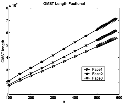
Figure 1: The average geodesic MST growth rates for three different face images in the Yale face database B.

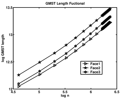
Figure 2: Log-log plot of Fig. 1.

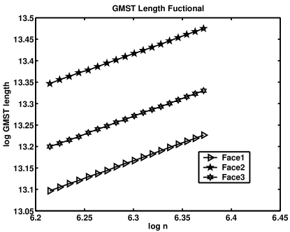
Figure 3: Blowup of Fig. 2 showing linearity of geodesic MST growth rates for large $n$.

In Fig. 1 the sequence of average GMST length functionals is plotted for each of the three faces. The symbols denote the locations of the 26 values of $n$ chosen for study and the corresponding values of the average GMST length. Note that the average GMST length sequences appear to increase almost linearly over $n$ for each of the three persons, albeit with different rate constants. However, after a log-log transformation, shown in Fig. 2, it becomes evident that the linear model for the of the mean GMST length functional is not valid for small $n$. Fig. 3 is a blowup of Fig. 2 for $n\geq 500$ and experimentally confirms the large-$n$ linear behavior predicted by Thm. 2 and supports the validity of the linear model (26).

Using the average GMST length sequences we next estimated slope and intercept parameters $a,b$ of the linear model and implemented the MOM estimator of dimension and entropy as described in the previous section. Only the range $n>500$ was used in fitting the linear model. The MOM estimator of $m$ was rounded to the nearest integer and the parameter $\beta_{m}$ was estimated by the large $m$ approximation [6]. The results are summarized in Table 3. As a result of this procedure the estimated face dimension $m$ was observed to vary between 5 and 6 for each of the individuals. The intrinsic entropy estimate expressed in log base 2 was concentrated around 70 bits. Note that as $\alpha=(m-1)/m$ is close to one for these estimated values of $m$ the estimates of $\alpha$-entropy are expected to be close to the Shannon entropy. These entropy estimates suggest that one should be able to get away with a model incorporating at most 6 parameters to describe the range 585 poses and illuminations of any of the three faces. An MDS ISOMAP analysis of the same three faces gave slightly higher estimates of dimension, varying between 6 and 7.

	Face1	Face2	Face3
$\hat{m}$	6	5	6
$\hat{H}$ (bits)	70.4	68.8	73.8

Table 3: Dimension estimates $\hat{m}$ and entropy estimates $\hat{H}$ for three faces in the Yale Face Database B.

6 Conclusion

We have presented a novel method for intrinsic dimension estimation and entropy estimation on smooth domain manifolds. With regards to intrinsic dimension estimation, the method proposed has two main advantages. First, it is global in the sense that tyhe MST is constructed over the entire and we thus avoid local linearizations. Second, unlike previous methods it simple to implement and does not require tuning any user-defined parameters such as eigenvalue thresholds or sizes of local neighborhoods. The GMST methods described in this paper are currently being applied to a large number of dimension reduction and entropy characterization problems including: gene clustering in bioinformatics, Internet traffic analysis, lung nodule classification, and radar signature analysis.

Acknowledgments

The authors acknowledge and thank the creators of Yale Face Database B for making their face image data publicly available (cvc.yale.edu/projects/yalefacesB/yalefacesB.html). The authors would also like to thank Huzefa Neemuchwala and Arpit Almal for their help in acquiring and processing these face images. This work was partially supported by the DARPA MURI program under ARO contract DAAD19-02-1-0262 and by the NIH Cancer Institute under grant 1PO1 CA87634-01. The authors can be contacted by email via jcosta,hero@eecs.umich.edu.

References

- [1] K. S. Alexander, “The RSW theorem for continuum percolation and the CLT for Euclidean minimal spanning trees,” Ann. Applied Probab., vol. 6, pp. 466–494, 1996.
- [2] F. Avram and D. Bertsimas, “The minimum spanning tree constant in geometrical probability and under the independent model: a unified approach,” Ann. Applied Probab., vol. 2, pp. 113–130, 1992.
- [3] J. Beardwood, J. H. Halton, and J. M. Hammersley, “The shortest path through many points,” Proc. Cambridge Philosophical Society, vol. 55, pp. 299–327, 1959.
- [4] M. Belkin and P. Niyogi, “Laplacian eigenmaps and spectral techniques for embedding and clustering,” in Advances in Neural Information Processing Systems, T. G. Diettrich, S. Becker, and Z. Ghahramani, editors, volume 14, MIT Press, 2002.
- [5] M. Bernstein, V. de Silva, J. C. Langford, and J. B. Tenenbaum, “Graph approximations to geodesics on embedded manifolds,” Technical report, Department of Psychology, Stanford University, 2000.
- [6] D. Bertsimas and G. van Ryzin, “An aysmptotic determination of the minimum spanning tree and minimum matching constants in geometrical probability,” Oper. Research Letters, vol. 9, pp. 223–231, 1990.
- [7] W. Boothby, An introduction to differentiable manifolds and Riemannian geometry, Academic, San Diego, Calif., rev. 2nd edition, 2003.
- [8] F. Camastra and A. Vinciarelli, “Estimating the intrinsic dimension of data with a fractal-based method,” IEEE Trans. on Pattern Analysis and Machine Intelligence, vol. 24, no. 10, pp. 1404–1407, October 2002.
- [9] M. Carmo, Differential geometry of curves and surfaces, Prentice-Hall, Englewood Cliffs, N.J., 1976.
- [10] M. Carmo, Riemannian geometry, Birkh user, Boston, 1992.
- [11] T. Cover and J. Thomas, Elements of Information Theory, Wiley, New York, 1991.
- [12] T. Cox and M. Cox, Multidimensional Scaling, Chapman & Hall, London, 1994.
- [13] I. Csiszar, “Generalized cutoff rates and Rényi’s information measures,” IEEE Trans. on Inform. Theory, vol. 41, no. 1, pp. 26–34, January 1995.
- [14] V. de Silva and J. B. Tenenbaum, “Unsupervised learning of curved manifolds,” in Nonlinear estimation and classification, D. Denison, M. H. Hansen, C. C. Holmes, B. Mallick, and B. Yu, editors, Springer-Verlag, New York, 2002.
- [15] V. de Silva and J. B. Tenenbaum, “Global versus local methods in nonlinear dimensionality reduction,” in Advances in Neural Information Processing Systems, MIT Press, 2003.
- [16] D. Donoho and C. Grimes, “Hessian eigenmaps: new locally linear embedding techniques for high dimensional data,” Technical Report TR2003-08, Dept. of Statistics, Stanford University, 2003.
- [17] A. Georghiades, P. Belhumeur, and D. Kriegman, “From few to many: Illumination cone models for face recognition under variable lighting and pose,” IEEE Trans. Pattern Anal. Mach. Intelligence, vol. 23, no. 6, pp. 643–660, 2001.
- [18] A. Gersho, “Asymptotically optimal block quantization,” IEEE Trans. on Inform. Theory, vol. 28, pp. 373–380, 1979.
- [19] H. Heemuchwala, A. O. Hero, and P. Carson, “Image registration using entropy measures and entropic graphs,” to appear in European Journal of Signal Processing, Special Issue on Content-based Visual Information Retrieval, Dec. 2003.
-
[20]
A. Hero, J. Costa, and B. Ma, “Convergence rates of minimal
graphs with random
vertices,” IEEE Trans. on Inform. Theory, vol. submitted, , 2002.
www.eecs.umich.edu/~hero/det_est.html. - [21] A. Hero, B. Ma, O. Michel, and J. Gorman, “Applications of entropic spanning graphs,” IEEE Signal Processing Magazine, vol. 19, no. 5, pp. 85–95, October 2002.
- [22] A. Hero and O. Michel, “Estimation of Rényi information divergence via pruned minimal spanning trees,” in IEEE Workshop on Higher Order Statistics, Caesaria, Israel, June 1999.
- [23] A. Hero and O. Michel, “Asymptotic theory of greedy approximations to minimal k-point random graphs,” IEEE Trans. on Inform. Theory, vol. IT-45, no. 6, pp. 1921–1939, Sept. 1999.
- [24] X. Huo and J. Chen, “Local linear projection (LLP),” in Proc. of First Workshop on Genomic Signal Processing and Statistics (GENSIPS), 2002.
- [25] A. K. Jain and R. C. Dubes, Algorithms for clustering data, Prentice Hall, Englewood Cliffs, NJ, 1988.
- [26] B. Kégl, “Intrinsic dimension estimation using packing numbers,” in Neural Information processing Systems: NIPS 02, 2002.
- [27] M. Kirby, Geometric Data Analysis : An Empirical Approach to Dimensionality Reduction and the Study of Patterns, Wiley-Interscience, 2001.
- [28] F. Memoli and G. Sapiro, “Fast computation of weighted distance functions and geodesics on implicit hyper-surfaces,” Journ. of Computationals Physics, no. 173, pp. 730–764, 2001.
- [29] F. Memoli, G. Sapiro, and S. Osher, “Solving variational problems and partial differentyial equations mapping into general target manifolds,” Technical Report 1827, IMA, January 2002.
- [30] H. Neemuchwala, A. O. Hero, and P. Carson, “Image matching using alpha-entropy measures and entropic graphs,” European Journal of Signal Processing (Special Issue on Content-based Visual Information Retrieval), To appear, 2003.
- [31] D. N. Neuhoff, “On the asymptotic distribution of the errors in vector quantization,” IEEE Trans. on Inform. Theory, vol. 42, pp. 461–468, March 1996.
- [32] S. Roweis and L. Saul, “Nonlinear dimensionality reduction by locally linear imbedding,” Science, vol. 290, pp. 2323.
- [33] J. M. Steele, Probability theory and combinatorial optimization, volume 69 of CBMF-NSF Regional Conferences in Applied Mathematics, Society for Industrial and Applied Mathematics (SIAM), 1997.
- [34] J. B. Tenenbaum, V. de Silva, and J. C. Langford, “A global geometric framework for nonlinear dimensionality reduction,” Science, vol. 290, pp. 2319–2323, 2000.
- [35] P. Verveer and R. Duin, “An evaluation of intrinsic dimensionality estimators,” IEEE Trans. on Pattern Analysis and Machine Intelligence, vol. 17, no. 1, pp. 81–86, January 1995.
- [36] J. E. Yukich, Probability theory of classical Euclidean optimization, volume 1675 of Lecture Notes in Mathematics, Springer-Verlag, Berlin, 1998.