Towards Modelling The Internet Topology – The Interactive Growth Model

Abstract

The Internet topology at the Autonomous Systems level (AS graph) has a power–law degree distribution and a tier structure. In this paper, we introduce the Interactive Growth (IG) model based on the joint growth of new nodes and new links. This simple and dynamic model compares favorable with other Internet power–law topology generators because it not only closely resembles the degree distribution of the AS graph, but also accurately matches the hierarchical structure, which is measured by the recently reported rich-club phenomenon.

1 INTRODUCTION

Faloutsos et al [1] discovered that the Internet topology at the Autonomous Systems (ASes) level (AS graph) has a power–law degree distribution, $P(k)\propto k^{-2.22}$, where node degree $k$ is the number of links a node has. Subramanian et al [2],using a heuristic argument based on the commercial relationship between ASes, found that the Internet has a tier structure. Tier 1 consists of a ‘core’ of ASes which are well connected to each other. Recently the rich–club phenomenon [3] was introduced as a quantitative metric to characterize the core tier without making any heuristic assumption on the interaction between network elements.

There are a number of Internet power–law topology generators, some are degree-based and others are structure-based. Tangmunarunkit et al [4] found that degree distributions produced by structure-based generators are not power–laws.

In this paper we introduce the Interactive Growth (IG) model based on the joint growth of new nodes and new links. We compare the AS graph against the IG model and three degree-based models, which are the Barabási and Albert (BA) scale–free model [5], the Inet–3.0 model [6] and the Generalized Linear Preference (GLP) model [7]. We show that the IG model compares favorable with other Internet power–law topology generators because it not only closely resembles the degree distribution of the AS graph, but also accurately matches the hierarchical structure measured by the rich-club phenomenon. The IG model is simple and dynamic, we believe it is a good step towards modelling the Internet topology.

2 RICH–CLUB PHENOMENON

Power–law topologies have a small number of nodes having large numbers of links. We call these nodes ‘rich nodes’. The AS graph shows a rich–club phenomenon [3], in which rich nodes are very well connected to each other and rich nodes are connected preferentially to the other rich nodes.

Recently the rich–club phenomenon was measured [3] in the so–called original–maps and extended–maps of the AS graph. The original–maps are based on the BGP routing tables collected by the University of Oregon Route Views Project [8]. The extended–maps [9] use additional data sources, such as the Looking Glass (LG) data and the Internet Routing Registry (IRR) data. The two maps have similar numbers of nodes, while the extended–maps have $40\%$ more links than the original–maps. The research showed the majority of the missing links in the original–maps are connecting links between rich nodes of the extended–maps, and therefore, the extended–maps show the rich–club phenomenon significantly stronger than the original–maps.

The rich-club phenomenon is relevant because the connectivity between rich nodes can be crucial for network properties, such as network routing efficiency, redundancy and robustness. For example in the AS graph, the members of the rich-club are very well connected to each other. This means that there are a large number of alternative routing paths between the club members where the average path length inside the club is very small (1 to 2 hops). Hence, the rich-club acts as a super traffic hub and provides a large selection of shortcuts. Network models without the rich-club phenomenon may under–estimate the efficiency and flexibility of the traffic routing in the AS graph. On the other hand, models without the rich-club phenomenon may over–estimate the robustness of the network to a node attack [10] where the removal of a few of its richest club members can break down the network integrity.

The rich–club phenomenon is a quantitatively simple way to differentiate the tier structures between power–law topologies and it provides a criterion for new network models.

3 DEGREE–BASED INTERNET TOPOLOGY GENERATORS

3.1 Inet–3.0 model

The Inet–3.0 model [6] was designed to match the measurements of the original–maps of the AS graph. The model is capable of creating networks with degree distribution similar to that of the measurements. The number of links generated by the model depends on two parameters, which are the total number of nodes and the percentage of nodes with degree one. The model typically generates 26% less links than the extended–AS graph.

3.2 Barabási–Albert (BA) model

The BA model [5] shows that a power–law degree distribution can arise from two generic mechanisms: 1) growth, where networks expand continuously by the addition of new nodes, and 2) preferential attachment, where new nodes are attached preferentially to nodes that are already well connected. The probability $\Pi(i)$ that a new node will be connected to node $i$ is proportional to $k_{i}$, the degree of node $i$.

$$\Pi(i)={k_{i}\over\sum_{j}k_{j}}$$ (1)

Using the mean–field theory, Barabási et al [11] estimated that the BA model generates networks with degree distribution of $P(k)\propto k^{-3}$. This model has generated great interests in various research areas and has been used as a starting point in the research of error and attack tolerance of the Internet [10].

3.3 Generalized Linear Preference (GLP) model

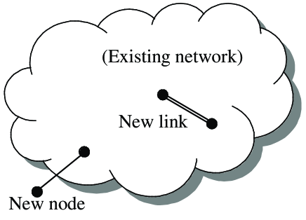
Figure 1: The growth of new nodes and new links are independent in the GLP model.

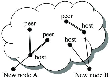
Figure 2: The growth of new nodes and new links are inter-dependant in the IG model.

The GLP model [7] was recently introduced. This model is a modification of the BA model. It reflects the fact that the evolution of the AS graph is mostly due to two operations, the addition of new nodes and the addition of new links between existing nodes. It starts with $m_{0}$ nodes connected through $m_{0}-1$ links. As shown in Figure 2, at each time–step, one of the following two operations is performed: 1) with probability $\rho\in[0,1],m<m_{0}$ new links are added between $m$ pairs of nodes chosen from existing nodes, and 2) with probability $1-\rho$, one new node is added and connected to $m$ existing nodes. The GLP model uses the generalized linear preference that the probability $\Pi(i)$ to choose node $i$ is

$$\Pi(i)={k_{i}-\beta)\over\sum_{j}(k_{j}-\beta)}$$ (2)

where the parameter $\beta\in(-\infty,1)$ can be adjusted such that nodes have a stronger preference of being connected to high degree nodes than predicted by the linear preference of the BA model (Equation 1). This model matches the AS graph (original–maps measured in Sept. 2000) in terms of the two characteristic properties of small–world networks [12], which are the characteristic path length and the clustering coefficient.

4 INTERACTIVE GROWTH (IG) MODEL

The Interactive Growth (IG) model also reflects the two main operations that account for the evolution of the AS graph, the addition of new nodes and the addition of new links. However the growth of links and nodes are inter-dependant in the IG model. As shown in Figure 2, at each time–step, a new node is connected to existing nodes (host nodes), and new links will connect the host nodes to other existing nodes (peer nodes). The IG model uses the same linear preference as the BA model (Equation 1) when choosing existing nodes to connect with.

In the actual Internet, new nodes bring new traffic load to its host nodes. This results in both the increase of traffic volume and the change of traffic pattern around host nodes and triggers the addition of new links connecting host nodes to peer nodes in order to balance network traffic and optimize network performance. We call the joint growth of new nodes and new links the Interactive Growth (IG).

The joint growth of new nodes and new links has two significant impacts, 1) rich nodes of the IG model are better inter-connected to each other than those of the BA model; and 2) rich nodes of the IG model have higher degrees than those of the BA model.

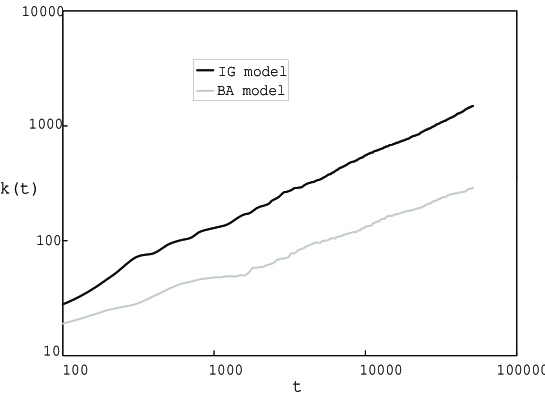
Figure 3: Time–evolution for node degree $k(t)$ against time $t$.

Figure 3 shows that the time–evolution of node degree in both the BA model and the IG model obeys a power–law $k(t)\propto t^{\theta}$ . As predicted by Barabási et al [11], $\theta$ of the BA model is $0.5$. Our calculation shows that $\theta$ of the IG model is $0.6$. This means that node degree in the IG model increases at a higher rate than in the BA model. The reason is that during the interactive growth of the IG model, host nodes not only connect to new nodes but also acquire new links connecting to peer nodes.

5 MODEL VALIDATION

As shown in Table 1, we generate 5 networks using the above four models with the same number of nodes as the AS graph, which in this paper is an extended–map measured on 26th May, 2001.

Table 1: Network properties

	$N$	$L$	$k_{max}$	$k_{average}$	$P(k=1)$	$P(k=2)$	$P(k=3)$
AS graph	11461	32730	2432	5.7	28.9%	40.3%	11.6%
IG model	11461	34363	842	6.0	26.0%	33.8%	10.5%
GLP(1)	11461	34363	517	6.0	68.4%	11.3%	5.1%
GLP(2)	11461	34363	524	6.0	52.0%	16.3%	7.9%
Inet–3.0	11461	24171	2010	4.2	40.0%	36.7%	8.2%
BA model	11461	34363	329	6.0	0%	0%	40.0%

$N$ – total number of nodes; $L$ – total number of links; $k_{average}$ – maximum degree; $k_{average}$ – average degree; $P(k)$ – degree distribution, percentage of nodes with degree $k$.

The GLP model(1) is grown with parameters of $\rho=0.66$, $m=1(m_{0}=10)$ and $\beta=0.6447$, which is recommended by authors of the model. The GLP model(2) is grown with the same parameters except $\beta=0$, which makes its generalized linear preference equivalent to the linear preference of the BA model.

The IG model starts with a random graph of $m_{0}=10$ nodes and $m_{0}$ links. In order to match the details of (low–range) degree distribution of the AS graph, at each time–step, 1) with 40% probability, a new node (as node $A$ shown in Figure 2) is connected to one host node and the host node is connected to two peer nodes; and 2) with 60% probability, a new node (as node $B$ shown in Figure 2) is connected to two host nodes and one of the host nodes is connected to one peer node. Thus, $m=3$ new links are added at every time–step.

5.1 DEGREE DISTRIBUTION

Degree distribution $P(k)$ is the percentage of nodes with degree $k$. It is reported [9] that, as shown in Figure 5, the degree distributions of the AS graph deviates significantly from a strict power law. To take this into consideration, we study the details of degree distribution by examining the low–range degree distribution ($k\leq 3$), the high–range degree distribution (1000 richest nodes) and the maximum degree, which is the largest number of links a node has.

5.1.1 Low–range degree distribution

The low–range degree distribution is important because nodes with degree one and two account for more than 70% of the total nodes of the AS graph. Furthermore in the AS graph, the percentage of nodes with degree one $P(1)$ is actually smaller than the percentage of nodes with degree two $P(2)$.

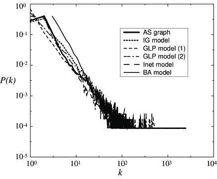
Figure 4: Degree distribution.

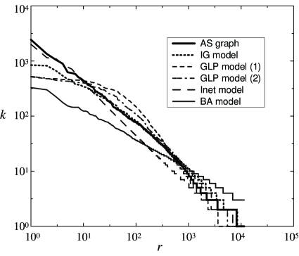
Figure 5: Node degree $k$ against rank $r$.

Figure 5 and Table 1 show that the IG model and the Inet–3.0 model closely match the low–range degree distribution of the AS graph. Only in the IG model, $P(1)$ is smaller than $P(2)$. Whereas, other models do not resemble the low–range degree distribution of the AS graph. For example, $P(1)$ of the GLP model (1) is as high as 68.4%.

5.1.2 High–range degree distribution

Figure 5 is a plot of node degree $k$ against node rank $r$, where $r$ is the rank of a node on a list sorted in a decreasing order of node degree. Figure 5 shows that the high–range degree distributions $(r\leq 10^{3})$ of the AS graph are quite different from those of the two GLP models and the BA model. The curve of the Inet-3.0 model significantly deviates from that of the AS graph between $r=10^{1}$ and $r=10^{3}$. Apart from the several richest nodes $(r\leq 10^{1})$, the IG model in general well matches the high–range degree distribution of the AS graph.

5.1.3 Maximum degree

The AS graph feature a large value of maximum degree ($k_{max}=2432$). As shown in Table 1, the GLP model (1) with parameter $\beta=0.6447$ and the GLP model(2) with $\beta=0$ (equivalent to linear preference) have similar maximum degrees (517/524). This suggests that, although the generalized linear preference of the GLP model (1) can make nodes have a stronger preference of being connected to high degree nodes, it does not effectively increase the maximum degree of the model.

The IG model uses the linear preference of the BA model. As we mention in Section 4 that due to the model’s interactive growth, the maximum degree of the IG model is significantly higher than that of the BA model and the two GLP models.

5.2 Rich–club phenomenon

The rich-club phenomenon is characterized by the rich-club connectivity, which measures the interconnection between rich nodes, and the node-node link distribution.

5.2.1 Rich–club connectivity

The maximum possible number of links between $n$ nodes is $n(n-1)/2$. The rich-club connectivity $\phi(r)$ is defined as the ratio of the actual number of links over the maximum possible number of links between nodes with rank less than $r$, where $r$ is normalized by the total number of nodes.

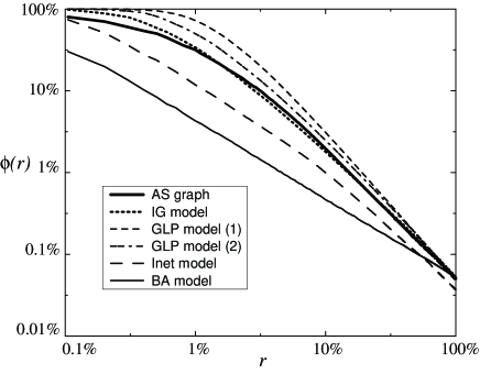
Figure 6: Rich–club connectivity $\phi(r)$ against node rank $r$.

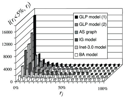
Figure 7: Node-node link distribution, number of link $l(r_{i}\leq 5\%,r_{j})$ against node rank $r_{j}$.

Figure 7 is a plot of the rich–club connectivity $\phi(r)$ against node rank $r$ on a log–log scale. The plot shows that only the IG model accurately matches the rich–club connectivity of the AS graph. The rich–club connectivity of the Inet–3.0 model and the BA model are significantly lower than that of the AS graph. This means that rich nodes in the two models are not as well connected to each other as in the AS graph. On the other hand, the rich–club connectivity of the two GLP models are significantly higher than that of the AS graph. This means the rich nodes in these two models are even more densely connected to each other than in the AS graph. To be specific, the AS graph and the IG model have $\phi(1\%)=32\%$, which indicates that the top 1% richest nodes have 32% of the maximum possible number of links connecting between them, comparing with $\phi(1\%)=18\%$ of the Inet–3.0 model, $\phi(1\%)=5\%$ of the BA model, $\phi(1\%)=72\%$ of the GLP model(1) and $\phi(1\%)=50\%$ of the GLP model(2).

5.2.2 Node-node link distribution

We define $l(r_{i},r_{j})$ as the number of links connecting nodes with node rank $r_{i}$ to nodes with $r_{j}$, where node ranks are normalized by the total number of nodes and $r_{i}\leq r_{j}$.

Table 2: Node–node link distribution

	AS graph	IG	GLP(1)	GLP(2)	Inet	BA
$L$	32730	34363	34363	34363	24171	34363
$l(r_{i}\leq 5\%)$	29602	26422	32376	29073	22620	15687
$l(r_{i}\leq 5\%,r_{j}\leq 5\%)$	8919	7806	16210	11540	3697	1511

$L$ – total number of links;
$l(r_{i}\leq 5\%)$ – number of links connecting with the top 5% rich nodes;
$l(r_{i}\leq 5\%,r_{j}\leq 5\%)$ – number of links connecting between the top 5% rich nodes.

Table 2 shows that the majority of links are the links connecting with the top $5\%$ rich node, $l(r_{i}\leq 5\%)$. Figure 7 illustrates more details by plotting $l(r_{i}\leq 5\%,r_{j})$ against corresponding node rank $r_{j}$, where $r_{j}$ is divided into $5\%$ bins.

The AS graph shows a rich–club phenomenon, in which rich nodes are connected preferentially to the other rich nodes. The number of links connecting between the top $5\%$ rich nodes ($l(r_{i}\leq 5\%,r_{j}\leq 5\%)=8919$) is significantly larger than the number of links connecting these rich nodes to other lower degree nodes.

The Inet–3.0 model does not show this phenomenon as strong as the AS graph. The BA model does not show this phenomenon at all, in stead, rich nodes are connected to nodes of all degrees with similar probabilities. On the contrary, the two GLP models show this phenomenon significantly stronger than the AS graph. In the GLP model(1), $l(r_{i}\leq 5\%,r_{j}\leq 5\%)=16210$ is nearly twice of that of the AS graph.

As seen from Figure 7, Table 2 and Figure 7, only the IG model accurately reproduce the rich–club phenomenon of the AS graph.

6 DISCUSSIONS AND CONCLUSIONS

The Inet–3.0 model is not a dynamic model. Although it well resembles the degree distribution, the model generates networks with typically 26% less links than the extended–AS graph. Figure 7 shows that the majority of the missing links are connecting links between the rich nodes of the AS graph. As a result, the Inet-3.0 model does not show the rich-club phenomenon as strong as the AS graph.

The BA model generates a strict power–law degree distribution, which is very different from that of the actual AS graph. Moreover, it does not show the rich–club phenomenon of the AS graph at all. This means that the network structure of the BA model is fundamentally different from that of the AS graph.

The reason for this is that, according to the dynamics of the BA model, all new links connect with new nodes. Due to the preferential attachment, the probability for a new node to become a rich node decreases as the network grows. This means that the number of links between rich nodes rarely increases after the initial growth. As a result, rich nodes are not well connected to each other, and in the end, they are connected to nodes of all degrees with similar probabilities. This result agrees with the study of Chen et al [9] which showed that from the available historical data, the AS graph does not evolves as the dynamics assumed in the BA model.

The GLP model does not reproduce the details of the degree distribution of the AS graph. It is interesting to notice that the rich–club phenomenon obtained from the GLP model is significantly stronger than the AS graph.

Tangmunarunkit et al [4] suggested that degree-based network topology generators can match the degree distribution and the hierarchy in real networks. Our results show that the degree-based models can generate networks with significantly different tier structures measured by the rich-club phenomenon.

The IG model compares favorable with other Internet power-law topology generators. It not only closely resembles the degree distribution of the AS graph, but also accurately matches the hierarchical structure of the AS graph. The IG model is a simple and dynamic model. The topological properties of the networks generated by the model are given by its joint growth of new nodes and new links.

It is possible to include other parameters in the IG model, such as bandwidth and delay. We expect the model to be used in simulation-based research for the Internet traffic engineering. We believe that the IG model is a good step towards modelling the Internet topology.

References

- [1] M. Faloutsos, P. Faloutsos, and C. Faloutsos, On Power–Law Relationship of the Internet Topology. Proc. of ACM SIGCOMM 1999.
- [2] L. Subramanian, S. Agarwal, J. Rexford and R. H. Katz, Characterizing the Internet Hierarchy from Multiple Vantage Points. Proc. of INFOCOM 2002.
- [3] S. Zhou and R. J. Mondragon, The missing links in the BGP–based AS connectivity maps. Proc. of PAM2003.
- [4] H. Tangmunarunkit, R. Govindan, S. Jamin, S. Shenker and W. Willinger, Network topology generators: Degree–based vs. structural. Proc. of ACM SIGCOMM 2002.
- [5] A. L. Barabási and R. Albert, Emergence of Scaling in Random Networks. Science, vol. 286, pp. 509–512, Oct. 1999.
- [6] J. Winick, and S. Jamin, Inet–3.0: Internet Topology Generator, Tech Report UM–CSE–TR–456–02. University of Michigan, 2002.
- [7] T. Bu and D. Towsley, On Distinguishing between Internet Power Law Topology Generators. Proc. of INFOCOM 2002.
- [8] University of Oregon, Route Views Project, http://www.routeviews.org.
- [9] Q. Chen, H. Chang, R. Govindan, S. Jamin, S. J. Shenker and W. Willinger, The Origin of Power Laws in Internet Topologies (Revisited). Proc. of IEEE INFOCOM 2002.
- [10] R. Albert, H. Jeong, and A. L. Barabási, Error and attack tolerance of complex networks. Nature, vol. 406, pp. 378–381, July 2000.
- [11] A. L. Barabási, R. Albert, and H. Jeong, Mean–field theory for scale–free random networks. Physica A, vol. 272, pp. 173–187, 1999.
- [12] D. J. Watts and S. H. Strogatz Collective dynamics of ‘small world’ networks, Nature, vol. 393, pp. 440–442, 1998.