Numerical Coverage Estimation for the Symbolic Simulation of Real-Time Systems

Abstract

Three numerical coverage metrics for the symbolic simulation of dense-time systems and their estimation methods are presented. Special techniques to derive numerical estimations of dense-time state-spaces have also been developed. Properties of the metrics are also discussed with respect to four criteria. Implementation and experiments are then reported.

Keywords: coverage, verification, symbolic simulation, real-time

1 Introduction

Presently, with verification and integration costs increasing to more than 50 percent of the development budget in real-world projects, it is more and more difficult to use traditional simulation technology to acquire enough trace coverage to confidently create system designs. As well, application of the new formal verification technology is still hampered by its intrinsic complexity. In the forseeable future, we expect that simulation and formal verification will be combined for verification of large-scale real-time systems. Symbolic simulation is such a combination[26]. It uses symbolic techniques[4, 8, 12, 17] of formal verification to represent space of simulation traces so that abstract (as opossed to concrete) behaviors can be observed in a trace. For verification of real-time systems, tools like UPPAAL[24] and RED[27, 28, 30, 31] support symbolic simulations.

Current symbolic simulation technology for real-time systems is still not as developed as that for untimed systems like Very Large Scale Integration (VLSI) Systems. For one thing, the important concept of coverage can be used to both estimate the value of a set of traces and to direct the generation of new traces. In short, coverage is how much has been verified of the target to be verified. The importance of this concept is that, in real-world projects, it is usually the case that we do not have enough resources to either run enough traces to obtain confidence, or to complete formal verification tasks. Product designs usually need to be released before we can obtain 100% confidence in the designs. Therefore it is important that we have some type of metric to evaluate confidence in our designs. A common coverage metric for simulation is code coverage, which measures the proportion of already-executed Hardware Description Language (HDL) statements during simulation. State and transition coverages are used in control state machines[19]. These coverage metrics have proven to be effective in bug escape reduction by pointing out coverage holes in the test suite. Coverage goals are used to measure the degree of confidence in the total verification effort, and to help the design team predict the optimal time for design release[5].

The coverage metrics used in traditional simulation, which is based on concrete traces, may not be directly applicable to the symbolic simulation of dense real-time systems, since there are infinitely many concrete traces and states for such systems. For example, the visited-state coverage metric[6, 25], which uses concrete reachable states in FSM to estimate coverage, is not suitable for the symbolic simulation of dense real-time systems. If we directly apply this coverage metric to the simulation of dense real-time systems, we will always have 0% coverage since the ratio of finitely many concrete states over the infinite reachable state-space is always zero.

To this end, we propose techniques to estimate numerical coverage for the symbolic simulation of dense real-time systems. As mentioned above, the states in such systems are dense, and the question follows that how do we count the states, since ”dense” stands for uncountable. Nevertheless, our techniques can estimate the covered proportion of the reachable state-space, and it is efficient and meanful. We approach the question by adopting the region-relation[2] to partition dense state-space, and propose a method to estimate the size of each proportion in section 6.2. We believe that our techniques can be used to help future development of various coverage-based verification techniques - including the design of new coverage metrics and coverage-based test-pattern generation - in real-time systems.

Before we can estimate numerical coverage, we must design a metric and its estimation procedure. This engenders the first research issue of this work, that is, how do we know if a metric is good ? In section 4, we present four criteria to serve as guidelines in coverage metric design. These criteria are: accountability (each basic portion of the target function is counted once and only once), coverability (100% coverage estimation is achievable), efficiency (the overhead in computing the coverage estimation is low), and discernment (risk states are discernable). According to these criteria, we adapt three coverage metrics from traditional testing research and development techniques to implement them in real-time systems. These three new metrics are: timed automata arc coverage metric(ACM), back-and-forth region coverage metric(RCM)[25], and triggering condition coverage metric(TCM). ACM is a straightforward adaptation from the technology of VLSI simulation, whereas RCM and TCM are not. For dense-time systems, RCM and TCM are more precise in the estimation of coverage by considering state-space coverage. We shall prove in a lemma that RCM has enough power to discern reachable risk states while ACM lacks sufficient power. To maintain the four criteria for dense-time state-spaces of real-time systems, we have developed techniques to quantitatively estimate the volume of a state-space, and to significantly prune irrelevant state-space portions from a verification task.

To demonstrate the usefulness of our techniques for real-world projects, in section 8, we have modeled and verified the Logical Link Control and Adaptation Layer Protocol(L2CAP) of Bluetooth specification[16]. Bluetooth is a widely adopted wireless communication standard in the industry. We model two devices that communicate with the Bluetooth L2CAP and carry out simulation experiments to gather data on numerical coverage estimation. We then compare the three coverage metrics with respect to our experiment data and the four criteria.

In section 2, we review related works. In section 3, we briefly present our verification framework with timed automata. In section 4, we discuss the four criteria for effective coverage metrics. In sections 5 through 7, we present our three coverage metrics and their estimation procedures. Finally, in section 8, we report on our experiment results with the Bluetooth L2CAP and discuss the implications of the experiment data.

2 Previous work

Coverage techniques have been widely discussed and applied in testing, simulation and formal verification of various system designs. In software testing, people use control flowgraphs [5], which are composed of processes, decisions, and junctions. Given a set of program stimuli, one can determine the statements activated by the stimuli with the coverage metrics of the flowgraphs. Programming code metrics measure syntactical characteristics of a code w.r.t its execution stimuli. For example, line coverage metric measures the number of distinct statements visited during the course of execution, branch coverage measures the number of distinct branch decisions, and path coverage measures the number of distinct paths (i.e. a unique combination of branch decisions and statements) exercised due to its execution stimuli[6]. The number of paths in a program may be exponentially related to program size which greatly hinders attaining 100% path coverage in software testing.

Coverage analysis techniques proposed for general HDL programs include: guaranteed coverage of every statement[9], transition coverage of a test set[20], and abstraction of models and semantic control over transition coverage[15]. Fallah provides OCCOM[14] to address the observability issue. Most of these HDL metrics are used to drive test-generation in simulation analysis.

Ho et al.[21] proposed a coverage metric to estimate the ”completeness” of a set of properties verified in model-checking FSM against a subset of CTL. A symbolic algorithm is also presented. Chockler et al.[10] also suggested several coverage metrics to measure completeness of a verified specification, and to find uncovered parts.

Dill proposed a way to bridge the gap between simulation and formal verification[13]. Generator of Test Cases for Hardware Architecture(GOTCHA) is a prototype coverage-driven test generator implemented as an extension to the Mur$\phi$ model-checker[23]. It supports state and transition coverage analysis in FSM. On completion of the entire reachable state-space enumeration, a random coverage task is chosen from those not yet covered.

Opposed to previous works with untimed or discrete-time systems, we apply coverage techniques in our symbolic simulator with dense-time model. One difficulty arises in the design of meaningful metrics to estimate state-spaces which are both dense and infinite. Traditional state and transition coverage metrics for untimed or discrete-time systems cannot be directly copied since metrics may always be zero based on the dense domain.

3 Framework of verification

3.1 System model

We use the widely accepted model of timed automata (TA)[2]. As we assume familiarity with this model, we will not go into much detail. A TA is a finite-state automaton equipped with a finite set of clocks which can hold nonnegative real-values. A TA can stay in only one mode (or control location) at a time. In operation, one transition can be triggered when its corresponding triggering condition is satisfied. Upon being triggered, the TA instantaneously transits from one mode to another and resets some clocks to zero. Between transitions, all clocks increase their readings at a uniform rate.

For convenience, given a set $Q$ of modes and a set $X$ of clocks, we use $B(Q,X)$ as the set of all Boolean combinations of mode predicate $\mbox{\tt mode}=q$, where mode is a special auxiliary variable, and inequalities of the forms $x-x^{\prime}\sim c$, where $q\in Q$, $x,x^{\prime}\in X\cup\{0\}$, “$\sim$” is one of $\leq,<,=,>,\geq$, and $c$ is an integer constant.

Definition 1

timed automata (TA):

A timed automaton $A$ is given as a tuple $\langle X,Q,I,\mu,T,\tau,\pi\rangle$ with the following restrictions: $X$ is the set of clocks, $Q$ is the set of modes, $I\in B(Q,X)$ is the initial condition on clocks, $\mu:Q\mapsto B(\emptyset,X)$ defines the invariance condition of each mode, $T\subseteq Q\times Q$ is the set of transitions, and $\tau:T\mapsto B(\emptyset,X)$ and $\pi:T\mapsto 2^{X}$ respectively define the triggering condition and the clock set to reset of each transition.     $\|$

A valuation of a set is a mapping from that set to another set. Given an $\eta\in B(Q,X)$ and a valuation $\nu$ of $X$, we say $\nu$ satisfies $\eta$, in symbols $\nu\models\eta$, iff $\eta$ will be evaluated true when the variables in $\eta$ are interpreted according to $\nu$.

Definition 2

states:

A state $\nu$ of $A=\langle X,Q,I,\mu,T,\tau,\pi\rangle$ is a valuation of $X\cup\{\mbox{\tt mode}\}$ such that

• $\nu(\mbox{\tt mode})\in Q$ is the mode of $A$ in $\nu$; and

• for each $x\in X$, $\nu(x)\in{\cal R}^{+}$ such that ${\cal R}^{+}$ is the set of nonnegative real numbers and $\nu\models\mu(\nu(\mbox{\tt mode}))$.     $\|$

For any $t\in{\cal R}^{+}$, $\nu+t$ is a state identical to $\nu$ except that for every clock $x\in X$, $\nu(x)+t=(\nu+t)(x)$. Given $\bar{X}\subseteq X$, $\nu\bar{X}$ is a new state identical to $\nu$ except that for every $x\in\bar{X}$, $\nu\bar{X}(x)=0$.

Definition 3

runs:

Given a timed automaton $A=\langle X,Q,I,\mu,T,\tau,\pi\rangle$, a run is an infinite sequence of state-time pairs $(\nu_{0},t_{0})(\nu_{1},t_{1})\ldots(\nu_{k},t_{k})\ldots$ such that $\nu_{0}\models I$ and $t_{0}t_{1}\ldots t_{k}\ldots$ is a monotonically increasing real-number (time) divergent sequence, and for all $k\geq 0$,

• for all $t\in[0,t_{k+1}-t_{k}]$, $\nu_{k}+t\models\mu(\nu_{k}(\mbox{\tt mode}))$; and

• either $\nu_{k}(\mbox{\tt mode})=\nu_{k+1}(\mbox{\tt mode})$ and $\nu_{k}+(t_{k+1}-t_{k})=\nu_{k+1}$; or

  • $(\nu_{k}(\mbox{\tt mode}),\nu_{k+1}(\mbox{\tt mode}))\in T$ and

  • $\nu_{k}+(t_{k+1}-t_{k})\models\tau(\nu_{k}(\mbox{\tt mode}),\nu_{k+1}(\mbox{\tt mode}))$ and

  • $(\nu_{k}+(t_{k+1}-t_{k}))\pi(\nu_{k}(\mbox{\tt mode}),\nu_{k+1}(\mbox{\tt mode}))=\nu_{k+1}$.     $\|$

3.2 Procedure of simulation and coverage analysis

We adopt the safety-analysis problem as our verification framework for simplicity. In this framework, we want to check whether an unsafe state can be reached by repetitive generation of symbolic traces. Formally speaking, a safety analysis problem instance consists of a timed automaton $A$ and a safety state-predicate $\eta\in B(Q,X)$. $A$ is safe with respect to $\eta$, in symbols $A\models\eta$, iff for all runs $(\nu_{0},t_{0})(\nu_{1},t_{1})\ldots(\nu_{k},t_{k})\ldots\ldots$, for all $k\geq 0$, and for all $t\in[0,t_{k+1}-t_{k}]$, $\nu_{k}+t\models\eta$, i.e., the safety requirement is guaranteed.

We construct our main procedure based on the well-discussed symbolic procedure, called next(), to compute a symbolic post-condition after a discrete transition and time-progress[17, 22]. Our symbolic simulation procedure takes the following form (details on coverage estimation in statements (1) and (4) will be explained in sections 5 through 7).   Symbolic_Simulate$(A,\eta)$ /* $A$ is a TA; $\eta$ is the safety state predicate. */ {
    Compute the numerical estimation $f$ of the whole target function $F$. (1)
    Let $\phi:=I$; $\phi^{\prime}:=\mbox{\em false}$; $v:=0$;
    While (true) {
       Let $\phi^{\prime}:=\phi;$
       Select a subspace $\psi$ of $\phi$ and a set $\bar{T}$ of transitions
           (possibly based on the value $\phi$ and $\bar{T}$); (2)
       Compute $\phi:=\phi\vee\bigvee_{e\in\bar{T}}{\tt next}(A,\psi,e)$; (3)
       Compute the estimation $v$ of the verified proportion $V$
           of the whole target function; (4)
       Print $v/f$ as the new numerical coverage estimation. (5)
       If $\phi\wedge\neg\eta\neq\emptyset$,
           print out ”a risk state is reachable” and exit;
       else if $v/f\geq threshold$,
           print out ”The threshold of the chosen coverage metric is reached” and exit;
       else $\phi=\phi^{\prime}$
           print out ”no risk states are found” and exit; (6)
    }
}  

In this manuscript, we use the term ”portion” to mean a basic unit of the target function in the estimation of trace coverage. Formally speaking, given a coverage metric, a portion is an equivalence class of (syntactic or semantic) entities of the target function in which two entities cannot be distinguished by the given coverage metric. The target function is conceptually defined as the set of all portions. Coverage means that how much of the target function has appeared in a set of simulation traces.

In the case of line coverage, a portion is a statement line. For state-coverage, a portion is a concrete state of the verification target. We can also use regions as the portion in the simulation of dense-time systems. In this case, a portion can contain infinitely many concrete states.

The target function can be the set of TA transitions (arcs), the regions of whole reachable state-space, or the regions of the triggering-conditions of all transitions in this paper.

In statement (2), we allow for the selection flexibility of various search strategies. Indeed, we have already implemented game-based, goal-oriented, and random strategies [31]. A subspace $\psi$ of the verified state-space $\phi$ and a set $\bar{T}$ of selected transitions are fed to procedure next() to compute the new next-step state-space after transitions and time-progress in statement (3). In statement (5), the coverage is numerically estimated as the ratio of the already-verified proportion of the whole target function. The infinite loop can continue until a risk state is reached, or until we feel that enough confidence has been established (coverage of the function has reached some specific $threshold$), or until we have reached the fixed point and finished the exhaustive search in statement (6).

However, our simulation framework is actually more general than simulation. For example, if in every iteration, we choose $\psi=\phi$ and $\bar{T}=T$ in statement (2), the whole procedure becomes a forward reachability analyzer. In the next few sections, we will discuss how to compute coverage estimations according to our three coverage metrics. As for the use of various strategies to guide searches, we believe it deserves more effort in the future.

4 Criteria for good coverage metrics

A good coverage estimation should tell us what proportion of a target function has been covered. We can partition a target function into portions and use an estimation function $\epsilon()$(from the set of portions to the set of nonnegative reals) to numerically estimate coverage. Formally speaking, $\epsilon:F\mapsto{\cal R}^{+}$ where ${\cal R}^{+}$ is the set of nonnegative reals. The whole target function can then be estimated as $f=\sum_{p\in F}\epsilon(p)$, and the current covered proportion $V$ of the target function, i.e. the verified subset of $F$, can be estimated as $v=\sum_{p\in V}\epsilon(p)$. In ACM, a portion represents a physical entity (i.e. a transition) of the automata, then coverage of that portion means that the physical entity has been used in some traces. In RCM and TCM, a portion represents a state subspace(i.e. a region), then the occurrence of any state in the portion along some simulation traces indicates the portion has been covered.

In practice, it can be difficult to design a good metric for dense-time systems. For example, we may want to use visited states as portions. Then in a dense-time state-space, we have to decide how a state should correspond to a portion. For discernment, a natural choice of a portion is the region presented in [2]. But it is very expensive (PSPACE-complete) to compute a precise representation of the entire reachable region set. A naive solution to this challenge is to use symbolic techniques with the popular data-structure of DBM (difference-bounded matrix)[12]. The challenge is that DBMs are not necessarily disjointed from one another. If we sum up portion estimations of each state-space using a DBM to calculate the total estimation, it is likely that some portions will be counted more than once.

After experimenting with various coverage metrics and their computation methods, we have identified the following four criteria for effective numerical coverage metrics.

• accountability: This assures that each portion of the target function is accounted for once and only once. If accountability is not maintained, we may run into the two following bizarre situations. First, some portions may not be accounted for and thus engineers simply cannot trust the metrics to check if all function portions have been covered. Second, it may happen that some portions are counted more than once and thus full coverage estimation is greater than 100% which makes no sense at all. Thus, accountability is the most important criterion. If we are going to use state-space or its abstraction to estimate coverage of target functions in dense-time systems, then we must develop new techniques, other than DBMs, to assure each portion is accounted for exactly once.

• coverability: This means that $\sum_{p\in V}\epsilon(p)=\sum_{p\in F}\epsilon(p)$ can be expected at the end of a symbolic simulation if enough traces have been generated. This is desirable in that 100% coverage can be the goal for verification. Moreover, if engineers decide to stop verification at 80% coverage, they can roughly estimate confidence in their products. It is likely to stump verification engineers if the coverage estimation converges at a small percentage number, no matter how many traces they have generated. One-hundred percent coverage can only be achieved if we have a precise numerical estimation of the entired target function $F$ to be verified.

• efficiency: This criterion measures the overhead in the computation of both the $f$ (at statement (1)) and the $v$ (at statement (4)) in procedure Symbolic_Simulate(). If complex formal reachability analysis is used to compute these two estimations, it is not worthwhile to estimate the coverage. In this work, we base our coverage estimation on transition-countings and state-space abstraction techniques and can efficiently calculate estimations in our three metrics.

• discernment: This criterion assesses the capability of a metric to discern risk states. This can be an issue when, in some metrics, risk states and non-risk states are likely to fall in the same $portion$. A metric that frequently fails to detect existing risk states at a high numerical coverage may give users unjustified and false confidence on their system designs.

The third and fourth criteria are kind of contradictory to each other. In a lot of cases, in order to discern risk states, we not only have to partition the portions intelligently, but we also have to partition them in great resolution. And this usually results in high complexity and low efficiency to reach high coverage with enough traces through the huge space of portions.

In the following, we shall use these four criteria to evaluate the coverage metrics presented in the next few sections.

5 TA arc coverage metric (ACM)

This is a straightforward adaptation from the technology of VLSI simulation and testing. In the computation of FSM arc coverage for VLSI, we conceptually transform a circuit to a finite-state automaton (FSM) and use the set of already-triggered transitions as $V$ and the set of executable transitions as $F$ to compute coverage estimation[6, 25]. The same definition of FSM arc coverage can readily be copied for the simulation of timed automata (TA). That is, we can also use the arcs of TAs to estimate coverage in the TA arc coverage metric (ACM). The straightforwardness of this metric has many desirable features. Each portion corresponds to an executable transition and the estimation function $\epsilon_{ACM}()$ maps everything to 1. The numerical estimation $f$ of the whole target function in statement (1) of procedure Symbolic_Simulate() can be $|T|$, the number of transitions in the TA. But it can be much tighter and more precise. In our implementation, we actually compute an untimed quotient structure of $A$’s state-space through forward analysis and eliminate those transitions that are actually not triggerible. In this way, we usually come up with a much smaller bound on $f$, which is the number of executable transitions in ACM.

As for the computation of the numerical coverage estimation $v$, we use $V$ as a static set variable of transitions such that $V=\emptyset$ initially. Each time when statement (4) in procedure Symbolic_Simulate() is executed, we perform the following two steps.   $V:=V\cup\bar{T}$; $v:=|V|$;  

LEMMA 1

ACM for dense-time systems satisfies the accountability criterion.

Proof : It is true since $\epsilon_{ACM}(e)=1$ for every executable transition in $F$, and we directly use the sizes of already-triggered and executable transition sets to calcualte the coverage.     $\|$

The criterion of full coverability is not guaranteed. But as can be seen from our experiment data in section 8, with a tight estimation of the set of executable transitions, it is possible to get very close to 100% of coverage. As for the criterion of efficiency, in each iteration, the overhead is a set-union operation and a size calculation of set and the efficiency is high. Finally, ACM may not have much discernment since a transition can very often be used in both a safe trace and a trace that ends in a risk state. This means ACM may reach 100% coverage without discovering the risk state even if it exists.

6 Back-and-forth region coverage metric (RCM)

ACM can very often be too coarse to discern risk states. Another extreme that can also be adapted from VLSI verification technology is the visited-state coverage metric[6, 25], which uses the reachable state set in FSM to estimate coverage. The challenge to incorporate the concept into our framework arises from the fact that in VLSI’s model, the states are discrete and countable while in timed automata, the states are dense and uncountable. A solution is to use equivalence classes in the dense-time state-space as portions. An equivalence relation to partition dense-time state-space is the region-equivalence relation between states[2]. In this paper, a region is a minimal state-space characterizable by a mode and clock-difference constraints in the form of $x-x^{\prime}\sim c$ where $x,x^{\prime}$ are two dense-time clocks, $\sim\in\{<,\leq,=,\geq,>\}$, and $c$ is an integer in the range of $[-C_{A:\eta},C_{A:\eta}]$ where $C_{A:\eta}$ is the biggest timing constant used in $A$ and the safety state predicate $\eta$. In this way, we consider in this section the concept of region coverage metric (RCM), in which a basic portion is a region, for the simulation of real-time systems. This coverage metric can have extra leverage with symbolic simulation since, in one step, we may generate a huge proportion of the state-space represented by a set of symbolic constraints.

There are three challenges in the implementation of RCM. First, how do we construct a tight estimation relevant to the reachability of the states? Second, how do we compute the coverage estimations of sets of portions, i.e. $\sum_{p\in V}\epsilon_{RCM}(p)$ and $\sum_{p\in F}\epsilon_{RCM}(p)$? Third, how do we maintain the accountability of the metrics? In this section, we counter these three challenges in three steps. For the first challenge, we use the intersection of abstractions of both backward and forward reachable state-space representations to construct a tight estimation of the whole target function (i.e., the whole reachable region set in RCM). For the second challenge, we work on the level of zones. A zone is a set of regions whose state-spaces are characterizable by a set of clock difference constraints. We then develop a procedure to calculate the region coverage estimation of a zone in the state-space. Our estimation is efficient, because we adopt the concept of region to partition the dense state-space and use CDD(Clock-Difference Diagram)[7] as our data structure. Many model-checkers for TAs are built around the central manipulation procedures of zones[1, 24, 27, 28, 30, 32]. Finally, for the third challenge, we present a data-structure and show that the data-structure can represent a state-space as a set of disjointed zones. With this data-structure, we can estimate the coverage of a state-space as the sum of coverages of a set of disjointed zones.

6.1 Tight estimation of the target function

In general, it is very expensive to compute representations for the exact reachable state-spaces. In our previous implementations, we use abstractions of either the backward or the forward reachable state-spaces to compute the estimation for the whole target function in RCM. But such estimations seem very imprecise. In some experiments, the final coverage estimations, when the whole reachable state-space representations have been constructed, fall in the range of $10^{-5}$. Moreover, much proportion of the reachable state-space seems irrelevant to the reachability from initial states to risk states.

We have observed that to analyze this reachability, we only have to trace through those states which are both backward reachable from a risk state and forward reachable from an initial state. So we use the following steps to compute an estimation of the whole target function.   Compute $F$ as the untimed quotient structure
        of the state-space of $A$ from initial states.
    Compute $B$ as the magnitude quotient structure
        of the backward reachable state-space of $A$ from risk states in $\neg\eta$.
    Let $F:=F\wedge B$;   In the second statement, we employ an abstraction technique, called magnitude abstraction, to compute the weakest preconditions from a state-predicate. A magnitude abstraction of a state-predicate eliminates from the state-predicate all clock inequalities like $x-x^{\prime}\sim c$ where $x,x^{\prime}$ are not zeros.

With these three steps, we have constrained $F$ to a much smaller state-space that is relevant to the reachability from initial states to risk states. Notice that these steps should not be regarded as extraneous expenses for RCM, since our symbolic simulator will initially take these steps to shrink the state-space that we have to search during the simulation anyway. According to our experiments reported in section 8, this technique has brought our ultimate estimation in RCM very close to 100% and resulted in much better coverability.

6.2 Coverage estimation of a zone

A zone is a state-space characterizable by a range constraints on the mode variable and a set of range constraints on the clock differences. Conveniently speaking, the characterization can be represented as a pair like $(Q^{\prime},K)$ such that

• $Q^{\prime}\subseteq Q$ and is the range of the mode variable; and

• $K$ is a set of range constraints like $c\sim x-x^{\prime}\sim^{\prime}c^{\prime}$ for clock differences, where $\sim,\sim^{\prime}\in\{<,\leq\}$ and $c,c^{\prime}\in[-C_{A:\eta},C_{A:\eta}]\cup\{-\infty,\infty\}$.

For the efficiency of coverage estimation, we intuitively compute something like a normalized volume estimation of zones. The volume estimation of a rectangular polyhedron in a multi-dimensional space can be computed as the multiplication of its length in each dimension. For efficiency, we intuitively interpret a zone as a rectangular polyhedron in a space of $1+|X|(1+|X|)$ dimensions. The range of variable mode’s value spans the first dimension while $x_{i}-x_{j}$, for each $x_{i},x_{j}\in X\cup\{0\}$ with $i<j$, spans a dimension. This intuitive and simplistic interpretation of zones neglects the fact that constraints on clock differences are not independent of one another. But our experiments show that it helps us design an efficient and coverable metric for region coverage.

In measuring the length of a clock difference constraint, we partition the real number lines into the following $4C_{A:\eta}+3$ basic intervals

$(-\infty,-C_{A:\eta})[-C_{A:\eta},-C_{A:\eta}]\ldots[-1,-1](-1,0)[0,0](0,1)[1,1](1,2)\ldots[C_{A:\eta},C_{A:\eta}](C_{A:\eta},\infty)$

and use the number of basic intervals covered by the clock difference constraint for the estimated length. For example, $-3\leq x-x^{\prime}<2$ has length $10$ because it covers $[-3,-3],(-3,-2),\ldots,[1,1],(1,2)$.

Such volume estimations can result in huge numbers not representable by integers in computers’ hardware. Thus instead of using the absolute length in each dimension to compute the estimated volume, we choose to use the normalized lengths (i.e. the floating point numbers of the length divided by the maximum length of the difference variables). The normalized length for $Q^{\prime}$ is thus $|Q^{\prime}|/|Q|$. The normalized length for a clock difference constraint is broken down to the following eight cases:

• $(2(c^{\prime}-c)+1)/(4C_{A:\eta}+3)$ for $c\leq x-x^{\prime}\leq c^{\prime}$ with $c\geq-C_{A:\eta}$ and $c^{\prime}\leq C_{A:\eta}$,

• $(2(c^{\prime}-c))/(4C_{A:\eta}+3)$ for either $c<x-x^{\prime}\leq c^{\prime}$ or $c\leq x-x^{\prime}<c^{\prime}$ with $c\geq-C_{A:\eta}$ and $c^{\prime}\leq C_{A:\eta}$,

• $(2(c^{\prime}-c)-1)/(4C_{A:\eta}+3)$ for $c<x-x^{\prime}<c^{\prime}$ with $c\geq-C_{A:\eta}$ and $c^{\prime}\leq C_{A:\eta}$,

• $(2(c^{\prime}+C_{A:\eta})+2)/(4C_{A:\eta}+3)$ for $-\infty<x-x^{\prime}\leq c^{\prime}$ with $c^{\prime}\leq C_{A:\eta}$,

• $(2(c^{\prime}+C_{A:\eta})+1)/(4C_{A:\eta}+3)$ for $-\infty<x-x^{\prime}<c^{\prime}$ with $c^{\prime}\leq C_{A:\eta}$,

• $(2(C_{A:\eta}-c)+2)/(4C_{A:\eta}+3)$ for $c\leq x_{1}-x_{1}^{\prime}<\infty$ with $c\geq-C_{A:\eta}$,

• $(2(C_{A:\eta}-c)+1)/(4C_{A:\eta}+3)$ for $c<x_{1}-x_{1}^{\prime}<\infty$ with $c\geq-C_{A:\eta}$,

• $1$ for $-\infty<x_{1}-x_{1}^{\prime}<\infty$; /* this case is usually not represented in zones */

Accordingly, the estimated normalized volume of a zone $(Q^{\prime},K)$ is

$\frac{|Q^{\prime}|}{|Q|}\cdot\Pi_{\mbox{\scriptsize"}c\sim x-x^{\prime}\sim^{\prime}c^{\prime}\mbox{\scriptsize"}\in K}(\mbox{the normalized length of }c\leq x-x^{\prime}\leq c^{\prime})$

6.3 Coverage estimation as a set of disjointed zones

Although the technique in the last subsection allows us to come up with a coverage estimation of a zone, the zones may intersect with one another and accountability may not be maintained. In this subsection, we present a representation for dense-time state-spaces such that zones represented are disjointed from one another. The representation that we have found with this property is CDD[7] with all zones in their closure forms (or all-pair shortest-path form). CDD is a BDD-like data-structure whose variables are clock differences like $x-x^{\prime}$ and whose outgoing arcs from variables are disjointed value ranges. For example, the CDD for the state-space of $(0-x_{1}\leq-3\wedge x_{1}-x_{3}<-4\wedge x_{2}-x_{1}<6)\vee(0-x_{2}<-1\wedge x_{2}-x_{1}<6)$ without terminal false is in figure 1.

Figure 1: CDD for $(0-x_{1}\leq-3\wedge x_{1}-x_{3}<-4\wedge x_{2}-x_{1}<6)\vee(0-x_{2}<-1\wedge x_{2}-x_{1}<6)$

Each path in this figure represents a zone in closure form. We refer interested readers to [7] for the definition and manipulations of CDD.

We can prove the following lemma.

LEMMA 2

Given a CDD with all zones in their closure forms, then each two paths in the CDD represent two disjointed zones.

Proof : From root to the terminals of the two paths, there is a branching node from which the two paths break away. The corresponding outgoing arcs from the node for the two paths are labeled with disjointed intervals. With the tightness of the zone constraints, this means that the zones of the two paths are disjointed.     $\|$

In our implementation, we follow the approach in [7] that a set of zones are first normalized to their closure forms before being stored in a CDD. Thus, for the convenience of presentation, we can assume that a CDD, say $D$, is represented as a true, or a false, or a tuple like $D=(x-x^{\prime},(\lambda_{1},D_{1}),\ldots,(\lambda_{n},D_{n}))$, such that

• the root node of $D$ is labeled with clock difference variable $x-x^{\prime}$.

• $\lambda_{1},\ldots,\lambda_{n}$ are disjointed intervals whose endpoints are in $\{-\infty,-C_{A:\eta},\ldots,-1,0,1,\ldots,C_{A:\eta},\infty\}$.

• for each $1\leq i\leq n$, the arc labeled with interval $\lambda_{i}$ points to $D_{i}$.

With the desirable feature of CDD, we can design the following symbolic procedure to compute the estimated volume of a state-space represented by CDD with all zones in closure forms.   normalized_volume$(D)$ /* $D$ is true, false, or $(x-x^{\prime},(\lambda_{1},D_{1}),\ldots,(\lambda_{n},D_{n}))$ */ {
    if $D$ is true, return 1; else if $D$ is false, return 0;
    else if $D$ is $(x-x^{\prime},(\lambda_{1},D_{1}),\ldots,(\lambda_{n},D_{n}))$, then
        return $\sum_{1\leq i\leq n}\frac{\mbox{the number of basic intervals covered by }\lambda_{i}}{4C_{A:\eta}+3}\mbox{\tt normalized\_volume}(D_{i})$;
}   Another advantage of this symbolic procedure is that we can take advantage of the data-sharing in CDD to avoid explicit enumeration of all disjointed zones. The normalized volume estimation of a substructure in a CDD can be saved and used for the estimation of other zones that use this same substructure.

6.4 Estimation of the region coverage

In our framework, both $V$ and $F$ in Symbolic_Simulate() on page 3.2 are conceptually represented as a set of pairs like $(Q^{\prime},D)$, for a state-space, where $D$ is a CDD with all zones in closure form, with the following constraints.

• For each two pairs $(Q_{1}^{\prime},D_{1}),(Q_{2}^{\prime},D_{2})$ in the set, $Q_{1}^{\prime}\cap Q^{\prime}_{2}=\emptyset$.

• For each pair $(Q^{\prime},D)$ in the set, $D$ represents the zones of all states with their modes in $Q^{\prime}$.

The procedure to transform a state-space representation in BDDs and DBMs to this representation can be found in [7]. Then at statement (4) of each iteration of procedure Symbolic_Simulate() on page 3.2, the estimated normalized volume $v$ for $V$ is $\sum_{(Q^{\prime},D)\in V}\frac{|Q^{\prime}|}{|Q|}\cdot\mbox{\tt normalized\_volume}(D)$ and $\frac{v}{f}=\frac{\sum_{(Q^{\prime},D)\in V}\frac{|Q^{\prime}|}{|Q|}\cdot\mbox{\tt normalized\_volume}(D)}{\sum_{(Q^{\prime},D)\in F}\frac{|Q^{\prime}|}{|Q|}\cdot\mbox{\tt normalized\_volume}(D)}$.

LEMMA 3

RCM satisfies the criterion of accountability.

Proof : According to lemma 2, zones respectively represented by paths in a CDD in its closure form are disjointed from one another. Thus in the algorithm of normalized_volume(), we count each portion once and only once and RCM satisfies the criterion of accountability.     $\|$

LEMMA 4

RCM satisifies the criterion of discernment, and it is impossible to reach 100% coverage without detecting the risk state, if any.

Proof : Given a timed automaton $A$ and a risk predicate $\eta$, in RCM, safe states and unsafe states are not in the same portion. This is because symbolic manipulations of zones are sufficient to answer the reachability problem of timed automata[2].     $\|$

According to lemma 4, RCM has enough discerning power to discover reachable risk states whereas ACM lacks such discerning power.

7 Triggering-condition coverage metric (TCM)

RCM has the advantage in accountability and discernment. But it may result in low coverability since our estimation of the reachable region sets can be imprecise. On the other hand, ACM can suffer from low discernment. In this section, we propose a balanced approach called triggering-condition coverage metric (TCM), in which we use the triggering conditions of all transitions as the body of the whole target function. TCM estimates the proportion of the covered triggering conditions of all transitions. It is accounted as the summation of triggering condition coverage for each transition. Formally speaking, a basic portion in TCM is a pair like $(e,\gamma)$ where $e$ is an executable transition and $\gamma$ is a region in subspace $\tau(e)$ (the triggering condition of $e$).

The numerical estimation $f$ of the whole target function in procedure Symbolic_Simulate() can be computed as $\sum_{e\in T}\mbox{\tt normalized\_volume}(\tau(e))$, where $\tau(e)$ is the triggering condition of each $e\in T$. We use $|T|$ variables, $V_{e}$ for each $e\in T$, to record the verified proportion of the triggering condition of each transition. Initially, for all $e\in T$, $V_{e}=\mbox{\em false}$. At each iteration’s execution of statement (4), we execute the following steps to compute the value $v$.   for each $e\in\bar{T}$, $V_{e}:=V_{e}\vee(\mbox{\tt abstract}_{e}(\phi\wedge\tau(e)))$;
    let $v:=\sum_{e\in T}\mbox{\tt normalized\_volume}(V_{e})$;   Here for the sake of efficiency, we use an abstract function $\mbox{\tt abstract}_{e}(d)$ to eliminate the recording of all clock difference variables not used in $\tau(e)$. For example, if $\tau(e)=0-x<-5\wedge x-y\leq 3$, then $\mbox{\tt abstract}_{e}(0-x<-7\wedge x-y\leq-2\wedge y-0\leq 2)=0-x<-7\wedge x-y\leq-2$ and the constraint literal $y-0\leq 2$ is filtered out since no constraint on difference $y-0$ is used in the triggering condition of $e$. Also in these two steps, we assume that while invoking $\mbox{\tt normalized\_volume}(V_{e})$ for each $e$, $V_{e}$ has already been transformed to the representation like $\{(Q^{\prime}_{1},D_{1}),\ldots,(Q^{\prime}_{n},D_{n})\}$.

It can be shown that TCM has the following desirable property.

LEMMA 5

TCM satisfies the criterion of accountability.

Proof : We calculate the normalized volume of zones based on the triggering conditions of transitions with TCM. Since zones of the triggering conditions of each transition represented by a CDD are disjointed, TCM satisfies the criterion of accountability.     $\|$

TCM is more efficient than the RCM since it is based on abstraction of zones whose representation complexity is usually lower. In the following experiments, we shall see that it satisfies the criterion of coverability without sacrificing its discernment.

8 Experiments with Bluetooth L2CAP

We have implemented our numerical coverage estimation techniques in our model-checker/simulator red 4.1. The input language of red is a set of communicating timed automata (CTA) that communicate with one another through CSP-style synchronization channels[18]. For each channel $\sigma$, two processes have to execute at the same instant to achieve a synchronization through the channel. In the synchronization instant, one process executes a transition with event $!\sigma$ for output and the other executes a transition with event $?\sigma$ for input.

To check the possibility of using our techniques in real-world projects, we have experimented with the Logical Link Control and Adaptation Layer Protocol(L2CAP) of Bluetooth specification[16]. The wireless communication standard of Bluetooth has been widely discussed and adopted in many appliances since it was published. L2CAP is layered over the Baseband Protocol and resides in the data link layer of Bluetooth. This protocol supports message multiplexing, packet segmentation and reassembly, and the conveying of quality of service information to the upper protocol layer. The protocol regulates the behavior between a master device and a slave device.

In our experiment, we collect coverage and performance data for L2CAP models both with and without design faults against various trace-generation strategies. In subsection 8.2, we report the coverage data of ACM, RCM, and TCM for the L2CAP model without faults. In subsection 8.3, we create six versions of the L2CAP model, each with an inserted fault, and report how the coverage metrics help us discern the faults before 100% coverage is reached. In appendix D, more coverage and performance data of our experiments with various trace-generation strategies can be found. Data is collected on a Pentium 4 with 1.7GHz, 256MB, running Red Hat Linux 7.0.

8.1 Modelling L2CAP

The L2CAP defines the actions performed by a master and a slave. A master is a device issuing a request while a slave is the one responding to the master’s request. A message sequence chart (MSC) that may better illustrate a typical scenario of event sequence in L2CAP can be found in appendix A. The scenario starts when the master’s upper layer issues an L2CA_ConnectReq (Connection Request) through the L2CA interface. Upon receiving the request, the master communicates the request through the unreliable network to the slave (with an L2CAP_ConnectReq), which will then convey the request to the slave’s upper layer (with an L2CA_ConnectInd).

The protocol goes on with messages bouncing back and forth until the master sends an L2CAP_ConfigRsp message to the slave. Then both parties can start exchanging data. Finally the master’s upper layer issues message L2CA_DisconnectReq to close the connection and the slave confirms the disconnection.

We use nine processes to model the entire activity in L2CAP. They are the master’s upper layer, the master’s L2CAP layer, master’s L2CAP time-out process, master’s L2CAP extended time-out process, the slave’s upper layer, the slave’s L2CAP layer, slave’s L2CAP time-out process, slave’s L2CAP extended time-out process, and the unreliable network. Each of these processes is described as a communicating timed automaton. The CTA for both the master and the slave can be found in appendix B. The safety condition is that when the master’s L2CAP layer stays in the OPEN state, the slave’s L2CAP layer can not enter the state W4_L2CA_DISCONNECT_RSP.

8.2 Coverage estimation when there is no fault

In this subsection, we execute procedure Symbolic_Simulate() with breadth-first strategy to verify our L2CAP model without faults. That is, each time we execute statement (2) in procedure Symbolic_Simulate(), we let $\bar{T}=T$ and $\phi=\psi$.

In each iteration, we calculate three estimations according to the three coverage metrics respectively. The data is in table 1.

iteration	ACM	ACM time	RCM	RCM time	TCM	TCM time
		overhead		overhead		overhead
1	4/97	0.00sec.	0.167816	7.39sec.	0.004092	0.02sec.
2	8/97	0.00sec.	0.173442	7.39sec.	0.382901	0.02sec.
3	12/97	0.00sec.	0.174279	7.40sec.	0.783131	0.02sec.
4	20/97	0.01sec.	0.175273	7.41sec.	0.799498	0.02sec.
5	36/97	0.02sec.	0.232154	7.41sec.	0.813138	0.03sec.
6	42/97	0.03sec.	0.295386	7.41sec.	0.815525	0.04sec.
7	64/97	0.05sec.	0.408160	7.42sec.	0.884971	0.06sec.
8	76/97	0.08sec.	0.561395	7.43sec.	0.920890	0.08sec.
9	88/97	0.12sec.	0.956820	7.44sec.	0.971241	0.11sec.
10	94/97	0.17sec.	0.965724	7.45sec.	0.975507	0.15sec.
11	94/97	0.22sec.	0.974428	7.46sec.	0.975507	0.18sec.
12	95/97	0.28sec.	0.975538	7.48sec.	0.976530	0.22sec.
13	97/97	0.34sec.	0.975783	7.49sec.	1.000000	0.26sec.
14	97/97	0.40sec.	0.981319	7.50sec.	1.000000	0.29sec.
15	97/97	0.47sec.	0.981338	7.52sec.	1.000000	0.33sec.
16	97/97	0.55sec.	0.982733	7.54sec.	1.000000	0.36sec.
17	97/97	0.63sec.	0.982734	7.56sec.	1.000000	0.40sec.
18	97/97	0.70sec.	0.982734	7.57sec.	1.000000	0.44sec.

Table 1: Coverage estimations and overheads with respect to iterations when there are no bugs

After 18 iterations, red 4.1 finishes the exhaustive search, and reports that the risk state is NOT reachable. It costs total cpu time 37.14 sec and memory usage 782k with ACM; total cpu time 30.59 sec and memory usage 632k with RCM; total CPU time 35.79 sec and memory usage 722k with TCM.

ACM and TCM can both reach 100% coverage estimation while RCM gets very close to 100%. The data shows that our methods have very high coverability in the experiment.

Another interesting thing is that for this correct L2CAP model, ACM and TCM can give us 100% confidence in their respective metrics before the whole reachable state-space representation is constructed. More precisely, according to ACM and TCM, we can stop at iteration 13 with 100% confidence. On the other hand, if we use straightforward formal verification, then we have to run through all the 18 iterations before we can conclude that the model is fault-free. This observation suggests that symbolic simulation with our coverage metrics can greatly save verification costs.

Since RCM gets us very close to 100% coverage, we can use 100% coverage as a goal for verification in RCM. More importantly, RCM is a better alternative in discernment than ACM and TCM. For one thing, at the 17th iteration, it could still increase to reflect more portions that have been traced through while ACM and TCM have already converged to 1.

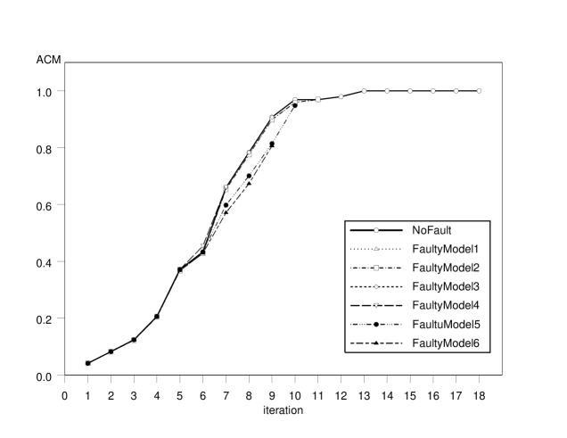
Figure 2: Growth of coverage with respect to iterations in ACM

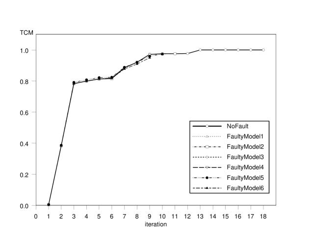
Figure 3: Growth of coverage with respect to iterations in TCM

As for the efficiency of our coverage estimation methods, we find that at the end of the state-space construction, the overhead incurred in the coverage estimation respectively for ACM, RCM and TCM is about 0.70, 7.57 and 0.44 seconds. Compared with the verification time, we find that for ACM, only $0.70/37.14\approx 0.01885=1.885\%$ of the verification CPU time is used in the coverage estimation. For TCM, only $0.44/35.79\approx 0.01229=1.229\%$ of the verification CPU time is used. This means that our implementation for both ACM and TCM are quite efficient. In figure 2 and figure 3, we drew the growth of coverage in ACM and TCM for the correct model and the six faulty models (details in the next subsection) with respect to the iterations. Notice that both coverage metrics grow quickly between the 4th iteration and the 10th iteration and then become flattened out to convergy to 100%. It reaches 100% at the 13th iteration and finishes the exhaustive search at the 18th iteration in the correct case. In the all faulty models we reach the risk state before the 11th iteration. The patterns show that both metrics may give engineers enough confidence to make decision quickly. For example, they may stop the simulation while the coverage becomes 100% or whilr it starts to converge 100%, and save the verification resources.

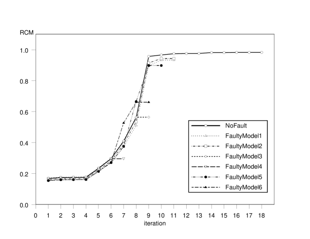
Figure 4: Growth of coverage with respect to iterations in RCM

For RCM, $7.57/30.59\approx 0.24747=24.747\%$ of the verification CPU time is used in the coverage estimation. A detail breakdown of the computation time shows that most of the overhead is consumed in the normalized volume calculation with the much larger CDD structure. This is the price of better discernment.

Figures 4 shows the growth of coverage in RCM for the same models. It’s interesting that the patterns dramatically increase in the first few iterations and then slow down in the next ierations. We can also detect the faults before the 11th iteration while the coverage in the correct model stops increasing in the 17th iteration and finishes the exhaustive search at iteration 18. Although RCM could not satisfy the coverability, we can figure out the end point while it stops increasing.

8.3 Coverage estimation when there is a fault

We design six L2CAP faulty models, each with an inserted fault. For convenience, we label these six faulty models with indices 1 through 6. In each faulty model, we change master or slave’s behaviors and let the risk condition become reachable. The description of the six faulty models are given in appendix C. We tried two trace-generation strategies. The first is breadth-first (see subsection 8.2). The second is depth-first. That is, at each time when we execute statement (2), we choose $\bar{T}$ to be of size 1 and only choose to fire one transition in $T$. We also keep a stack so that we can backtrack to previous iterations to choose an alternative transitions at statement (2). The coverage data is shown in table  2.

Strategy	Faulty Models	Depth	ACM	RCM	TCM	Risk state reached?
Depth	1	66	71/98	0.355262	0.958950	Yes
First	2	64	71/98	0.354993	0.958950	Yes
	3	26	27/97	0.293884	0.437878	Yes
	4	96	90/97	0.924978	0.963982	Yes
	5	64	63/97	0.355688	0.948209	Yes
	6	62	61/98	0.357885	0.936412	Yes
Breath	1	11	95/98	0.932724	0.975532	Yes
First	2	11	95/98	0.943274	0.975532	Yes
	3	9	88/97	0.564228	0.971241	Yes
	4	7	64/97	0.294859	0.884971	Yes
	5	10	92/97	0.898077	0.973172	Yes
	6	9	79/98	0.660754	0.949243	Yes

Table 2: Coverage estimations with respect to two strategies for the 6 faulty models

The most interesting thing in table 2 is that the faults are all detected before we reach 100% coverage. This means that our three coverage metrics have enough discernment for the six faulty models.

9 Conclusion

Symbolic simulation combines the advantages of both simulation and formal verification and can be an important verification approach before fully automatic formal verification becomes applicable. In this paper, we present techniques for coverage estimation for dense-time systems. We hope such techniques can be the solid stepstone toward the development of powerful symbolic simulators for industry real-time systems. Many issues raised in this work also deserve future research. For example, it will be interesting to see the design of quantitative metrics for our criterion of discernment in the symbolic simulation of dense-time systems. With such metrics, the criterion becomes equivalent to the notion of observability[11].

APPENDICES

Appendix A Message sequence chart for Bluetooth L2CAP

Figure 5: A message sequence chart of L2CAP

The two outer descriptions represent the states of L2CAP layers.

Appendix B Bluetooth L2CAP

Figure 6: CTA of a Bluetooth device

Appendix C Description of the six faulty models

All faulty models lead the risk state reachable and violate the safety condition. Recall that the safety condition is that while master L2CAP device still stays in the OPEN state at the time, the slave L2CAP device may not enter the W4_L2CA_DISCONNECT_RSP state. We compare the fault and correct behaviors of these faulty models as below:

• $\mbox{\tt Faulty Model1}:$ The slave will enter into W4_L2CA_DISCONNECT_RSP state while receiveing master’s data from network and notifying upper layer. In the correct model, the slave shall stay in OPEN state.

• $\mbox{\tt Faulty Model2}:$ The slave will leave OPEN state and enter into W4_L2CA_DISCONNECT_RSP state while reciveing upper layer’s disconnect command, sending this request to master through network, and starting the timer. In the correct model, the slave shall leave OPEN state and enter into W4_L2CAP_DISCONNECT_RSP state to wait for the master’s response from network.

• $\mbox{\tt Faulty Model3}:$ The master remains staying in OPEN state while reciveing upper layer’s disconnect command, sending this request to slave through network, and starting the timer. In the correct model, the master shall leave OPEN state and enter into W4_L2CAP_DISCONNECT_RSP state to wait for the slave’s response from network.

• $\mbox{\tt Faulty Model4}:$ The master will leave CONFIG state and enter into OPEN state while reciveing upper layer’s disconnect command, sending this request to slave through network, and starting the timer. In the correct model, the master shall enter into W4_L2CAP_DISCONNECT_RSP state to wait for the slave’s response from network.

• $\mbox{\tt Faulty Model5}:$ The slave will leave CONFIG state and enter into W4_L2CAP_DISCONNECT_RSP state while receiving upper layer’s configuration response and having received master’s response. In the correct mode, the slave shall leave CONFIG state and enter into OPEN state after finishing the configuration process.

• $\mbox{\tt Faulty Model6}:$ The slave will leave CONFIG state and enter into W4_L2CAP_DISCONNECT_RSP state while receiving upper layer’s configuration response but not yet having received master’s response. In the correct mode, the slave should stay in CONFIG state since it doesn’t finish the configuration process.

Appendix D Coverage estimation with various search strategies

It is also interesting to see how our techniques can be used together with various trace-generation strategies in symbolic simulation. We only briefly describe the trace-generation strategies that we have implemented for our experiments in the following.

• Random Walk Strategy: Each time we execute statement (2), red 4.1 randomly choose a firable transition to be the sole element in $\bar{T}$.

• Game-based Strategy: We use the term ”game” here because we envision the concurrent system operation as a game. Users can specify some processes to be treated as players while the other processes are treated as opponents. At each time we execute statement (2), we either randomly choose a firable transition from the opponent processes or choose $\bar{T}$ to be the set of all firable transitions of the player processes. In this strategy, we alternately execute sequences of all players’ transitions and sequences of a random-walk of the opponents’ transitons. In this experiment, we view all processes whose local variables and clocks appear in the safety predicate as players. All other processes are opponents.

• Goal-oriented Strategy: According to this strategy, heuristics are designed for the choice of a single transition in each execution of statement (2) in the hope that a short trace leading to a risk state can be constructed.

Our coverage data with the generation of a single symbolic trace is in table 3.

Strategy	Faulty Models	Depth	ACM	RCM	TCM	Risk state reached?
Random	1	21	34/98	0.437014	0.623092	No
Walk	2	11	23/98	0.181328	0.423497	No
	3	11	22/97	0.172719	0.411343	No
	4	8	26/97	0.168460	0.217365	No
	5	30	44/97	0.294042	0.839828	No
	6	19	27/98	0.179093	0.636663	No
Goal	1	15	19/98	0.187034	0.613695	No
Oriented	2	14	12/98	0.164324	0.597204	No
	3	8	26/97	0.169848	0.217365	No
	4	13	12/97	0.199808	0.597815	No
	5	14	28/97	0.157394	0.613456	No
	6	19	19/98	0.163539	0.613695	No
Game	1	14	30/98	0.429387	0.421141	No
Based	2	8	26/98	0.160757	0.217143	No
	3	23	33/97	0.309106	0.631373	No
	4	17	29/97	0.188423	0.429172	No
	5	20	32/97	0.183961	0.626350	No
	6	24	20/98	0.158451	0.798677	No

Table 3: Coverage estimations with respect to automatic trace generation strategies for the 6 faulty models

The experiments shows that it is viable to integrate our techniques with other verification and simulation techniques.

References

- [1] R. Alur. Timed Automataa CAV’99, LNCS 1633, Springer-Verlag, pp. 8-22.
- [2] R. Alur, C. Courcoubetis, D.L. Dill. Model Checking for Real-Time Systems, IEEE LICS, 1990.
- [3] R. Alur, D.L. Dill. Automata for modelling real-time systems. ICALP’ 1990, LNCS 443, Springer-Verlag, pp. 322-335.
- [4] J.R. Burch, E.M. Clarke, K.L. McMillan, D.L. Dill, L.J. Hwang. Symbolic Model Checking: States and Beyond, IEEE LICS, 1990.
- [5] B.Beizer. Software Testing Techniques. Van Nostrand Rheinhold, New York, 2nd ed., 1990.
- [6] L. Bening, H. Foster. Principles of Verifiable RTL Design, a Functional Coding Style Supporting Verification Processes in Verilog, 2nd ed., Kluwer Academic Publishers, 2001.
- [7] G. Behrmann, K.G. Larsen, J. Pearson, C. Weise, Wang Yi. Efficient Timed Reachability Analysis Using Clock Difference Diagrams. CAV’99, July, Trento, Italy, LNCS 1633, Springer-Verlag.
- [8] R.E. Bryant. Graph-based Algorithms for Boolean Function Manipulation, IEEE Trans. Comput., C-35(8), 1986.
- [9] K-T. Cheng and A. S. Krishnakumar. Automatic Functional Test Generation Using the Extended Finite State Machine Model. In Proceedings of the 30th Design Automation Conference, pp. 86-91, June 1993.
- [10] Hana Chockler, Orna Kupferman, Moshe Y. Vardi. Coverage Metrics for Temporal Logic Model Checking. LNCS 2031, pp. 528-552, 2001.
- [11] S. Devadas, A. Ghosh, K. Keutzer. An Obervability-Based Code Coverage Metric for Functional Simulation. IEEE ICCAD’96.
- [12] D.L. Dill. Timing Assumptions and Verification of Finite-state Concurrent Systems. CAV’89, LNCS 407, Springer-Verlag.
- [13] D.L. Dill. What’s Between Simulation and Formal Verification? In Proceedings of DAC1998.
- [14] Farzan Fallah, Srinivas Devadas, Kurt Keutzer. OCCOM: Efficient Computation of Observability-Based Code Coverage Metrics for Functional Verification. Design Automation Conference, pp. 152-157, 1998.
- [15] D. Geist, M. Farkas, A. Landver, Y.Lichtenstein, S. Ur, Y. Wolsfthal. Coverage-Directed Test Generation Using Symbolic Techniques. In Proceedings of the Int’l Conference on Formal Methods in CAD, November 1996.
- [16] J. Haartsen. Bluetooth Specification, version 1.0. http://www.bluetooth.com/
- [17] T.A. Henzinger, X. Nicollin, J. Sifakis, S. Yovine. Symbolic Model Checking for Real-Time Systems, IEEE LICS 1992.
- [18] C.A.R. Hoare. Communicating Sequential Processes, Prentice Hall, 1985.
- [19] Y. Hoskote, D.Moundanos, J. Abraham. Automatic Extraction of the Control Flow Machine and Application to Evaluating Coverage of Verification Vectors. Proceedings of ICCD, pp. 532-537, October 1995.
- [20] Y. Hoskote, D. Moundanos, and J. A. Abraham. Automatic Extraction of the control flow machine and application to evaluating coverage of verification vectors. In Proceedings of the Int’l Conference on Computer Design, pp 532-537, October 1995.
- [21] Y. Hoskote, T. Kam, P.-H. Ho, and X. Zhao. Coverage estimation for symbolic model checking. In Proceedings of DAC1999, pp. 300-305.
- [22] Kim G. Larsen, Paul Pettersson and Wang Yi. Model-Checking for Real-Time Systems. In Proceedings of the 10th International Conference on Fundamentals of Computation Theory, Dresden, Germany, August 22-25, 1995. LNCS 965, pp. 62-88, Horst Reichel.
- [23] B. Mike, G. Daniel, H. Alan, W. Yaron, M. Gerard, S. Ralph. A Study in Coverage-Driven Test Generation. In Proceedings of DAC1999, pp. 970-975.
- [24] P. Pettersson, K.G. Larsen. UPPAAL2k. In Bulletin of the European Association for Theoretical Computer Science, Vol. 70, pp. 40-44, 2000.
- [25] P. Rashinkar, P. Paterson, L. Singh. System-on-a-chip Verification, Methodology and Techniques. Kluwer Academic Publishers, 2001.
- [26] C.-J.H. Seger, R.E. Bryant. Formal Verification by Symbolic Evaluation of Partially-Ordered Trajectories. Formal Methods in System Designs, Vol. 6, No. 2, pp. 147-189, Mar. 1995.
- [27] F. Wang. Efficient Data-Structure for Fully Symbolic Verification of Real-Time Software Systems. TACAS’2000, March, Berlin, Germany. LNCS 1785, Springer-Verlag.
- [28] F. Wang. Symbolic Verification of Complex Real-Time Systems with Clock-Restriction Diagram, to appear in Proceedings of FORTE, August 2001, Cheju Island, Korea.
- [29] F. Wang. Efficient Verification of Timed Automata with BDD-like Data-Structures. to appear in proceedings of VMCAI 2003, New York City, USA, Jan. 2003. LNCS, Springer-Verlag.
- [30] F. Wang. Efficient Verification of Timed Automata with BDD-like Data-Structures. to appear in proceedings of VMCAI 2003, New York City, USA, Jan. 2003. LNCS, Springer-Verlag.
- [31] F. Wang, G-D. Hwang, F. Yu. Symbolic Simulation of Real-Time Concurrent Systems to appear in proceedings of RTCSA 2003, Tainan, Taiwan. Feb. 2003. LNCS, Springer-Verlag;
- [32] S. Yovine. Kronos:A Verification Tool for Real-Time Systems. International Journal of Software Tools for Technology Transfer, Vol. 1, Nr. 1/2, October 1997.