Approximate analysis of search algorithms with “physical” methods

Abstract

An overview of some methods of statistical physics applied to the analysis of algorithms for optimization problems (satisfiability of Boolean constraints, vertex cover of graphs, decoding, …) with distributions of random inputs is proposed. Two types of algorithms are analyzed: complete procedures with backtracking (Davis-Putnam-Loveland-Logeman algorithm) and incomplete, local search procedures (gradient descent, random walksat, …). The study of complete algorithms makes use of physical concepts such as phase transitions, dynamical renormalization flow, growth processes, … As for local search procedures, the connection between computational complexity and the structure of the cost function landscape is questioned, with emphasis on the notion of metastability.

I Introduction

The computational effort needed to deal with large combinatorial structures considerably varies with the task to be performed and the resolution procedure usedpapadimi . The worst case complexity of a task, more precisely an optimization or decision problem, is defined as the time required by the best algorithm to treat any possible inputs to the problem. For instance, the sorting problem of a list of $N$ numbers has worst-case complexity $\sim N\log N$: there exists several algorithms that can order any list in at most $\sim N\log N$ elementary operations, and none with asymptotically less operations. Unfortunately, the worst-case complexities of many important computational problems, called NP-Complete, is not known. Partitioning a list of $N$ numbers in two sets with equal partial sums is one among hundreds of such NP-complete problems. It is a fundamental conjecture of theoretical computer science that there exists no algorithm capable of partitioning any list of length $N$, or of solving any other NP-Complete problem with inputs of size $N$, in a time bounded by a polynomial of $N$. Therefore, when dealing with such a problem, one necessarily uses algorithms which may takes exponential times on some inputs. Quantifying how ‘frequent’ these hard inputs are for a given algorithm is the question answered by the analysis of algorithms. In this paper, we will present an overview of recent works done by physicists to address this point, and more precisely to characterize the average performances, called hereafter complexity, of a given algorithm over a distribution of inputs to an optimization problem.

The history of algorithm analysis by physical methods/ideas is at least as old as the use of computers by physicists. One well-established chapter in this history is, for instance, the analysis of Monte Carlo sampling algorithms for statistical mechanics models. In this context, it is well known that phase transitions, i.e. abrupt changes in the physical properties of the model, can imply a dramatic increase in the time necessary to the sampling procedure. This phenomenon is commonly known as critical slowing down. The physicists’ insight in this problem comes mainly from the analogy between the dynamics of algorithms and the physical dynamics of the system. This analogy is quite natural: in fact many algorithms mimick the physical dynamics itself.

A quite new idea is instead to abstract from physically motivated problems and use statistical mechanics ideas for analyzing the dynamics of algorithms. In effect there are many reasons which suggest that analysis of algorithms and statistical physics should be considered close relatives. In both cases one would like to understand the asymptotic behavior of dynamical processes acting on exponentially large (in the size of the problem) configuration spaces. The differences between the two disciplines mainly lie in the methods (and, we are tempted to say, the style) of investigation. Theoretical computer science derives rigorous results based on probability theory. However these results are sometimes too weak for a complete characterization of the algorithm. Physicists provide instead heuristic results based on intuitively sensible approximations. These approximations are eventually validated by a comparison with numerical experiments. In some lucky cases, approximations are asymptotically irrelevant: estimates are turned into conjectures left for future rigorous derivations.

Perhaps more interesting than stylistic differences is the point of view which physics brings with itself. Let us highlight two consequences of this point of view.

First, a particular importance is attributed to “complexity phase transitions” i.e. abrupt changes in the resolution complexity as some parameter defining the input distribution is variedAI ; Friedgut . We shall consider two examples in the next Sections:

• Random Satisfiability of Boolean constraints (SAT). In $K$-SAT one is given an instance, that is, a set of $M$ logical constraints (clauses) among $N$ boolean variables, and wants to find a truth assignment for the variables which fulfill all the constraints. Each clause is the logical OR of $K$ literals, a literal being one of the $N$ variables or its negation e.g. $(x_{1}\vee x_{17}\vee\overline{x_{31}})$ for 3-SAT. Random $K$-SAT is the $K$-SAT problem supplied with a distribution of inputs uniform over all instances having fixed values of $N$ and $M$. The limit of interest is $N,M\to\infty$ at fixed ratio $\alpha=M/N$ of clauses per variableMit ; Hans .

• Vertex cover of random graphs (VC). An input instance of the VC decision problem consists in a graph $G$ and an integer number $X$. The problem consists in finding a way to distribute $X$ covering marks over the vertices in such a way that every edge of the graph is covered, that is, has at least one of its ending vertices marked. A possible distribution of inputs is provided by drawing random graphs $G$ à la Erdös-Renyì i.e. with uniform probability among all the graphs having $N$ vertices and $E$ edges. The limit of interest is $N,E\to\infty$ at fixed ratio $c=2E/N$ of edges per vertex.

The algorithms for random SAT and VC we shall consider in the next Sections undergo a complexity phase transition as the input parameter $\pi$ ($=\alpha$ for SAT, $c$ for VC) crosses some critical threshold $\pi_{\rm alg}$. Typically resolution of a randomly drawn instance requires linear time below the threshold $\pi<\pi_{\rm alg}$ and exponential time above $\pi>\pi_{\rm alg}$. The observation that most difficult instances are located near the phase boundary confirms the relevance of the phase-transition phenomenon.

Secondly, a key role is played by the intrinsic (algorithm independent) properties of the instance under study. The intuition is that, underlying the dramatic slowing down of a particular algorithm, there can be some qualitative change in some structural property of the problem e.g. the geometry of the space of solutions. While there is no general understanding of this question, we can further specify the above statements case-by-case. Let us consider, for instance, a local search algorithm for a combinatorial optimization problem. If the algorithm never increases the value of the cost function $F(C)$ where $C$ is the configuration (assignment) of variables to be optimized over, the number and geometry of the local minima of $F(C)$ will be crucial for the understanding of the dynamics of the algorithm. This example is illustrated in Sec. III.3. While the “dynamical” behavior of a particular algorithm is not necessarily related to any “static” property of the instance, this approach is nevertheless of great interest because it could provide us with some ‘universal’ results. Some properties of the instance, for example, may imply the ineffectiveness of an entire class of algorithms.

While we shall mainly study in this paper the performances of search algorithms applied to hard combinatorial problems as SAT, VC, we will also consider easy, that is, polynomial problems as benchmarks for these algorithms. The reason is that we want to understand if the average hardness of resolution of solving NP-complete problems with a given distribution of instances and a given algorithm truly reflects the intrinsic hardness of these combinatorial problems or is simply due to some lack of efficiency of the algorithm under study. The benchmark problem we shall consider is random XORSAT. It is a version of a satisfiability problem, much simpler than SAT from a computational complexity point of viewCrei . The only but essential difference with SAT is that a clause is said to be satisfied if the exclusive, and not inclusive, disjunction of its literals is true. XORSAT may be recast as a linear algebra problem, where a set of $M$ equations involving $N$ Boolean variables must be satisfied modulo 2, and is therefore solvable in polynomial time by various methods e.g. Gaussian elimination. Nevertheless, it is legitimate to ask what are the performances of general search algorithms for this kind of polynomial computational problem. In particular, we shall see that some algorithms requiring exponential times to solve random SAT instances behave badly on random XORSAT instances too. A related question we shall focus on in Sec. III.2 is decoding, which may also, in some cases, be expressed as the resolution of a set of Boolean equations.

The paper is organized as follows. In Sec. II.1 we shall review backtracking search algorithms, which, roughly speaking, work in the space of instances. We explain the general ideas and then illustrate them on random SAT (Sec. II.2) and VC (Sec. II.3). In Sec. II.4 we consider the fluctuations in running times of these algorithms and analyze the possibility of exploiting these fluctuations in random restart strategies. In Sec. III we turn to local search algorithms, which work in the space of configurations. We review the analysis of such algorithms for decoding problems (Sec. III.2), random XORSAT (Sec. III.3), and SAT (Sec. III.4). Finally in the Conclusion we suggest some possible future developments in the field.

II Analysis of the Davis-Putnam-Loveland-Logeman search procedure

II.1 Overview of the algorithm and physical concepts

In this section, we briefly review the Davis-Putnam-Loveland-Logemann (DPLL) procedure DP ; survey . A decision problem can be formulated as a constrained satisfaction problem, where a set of variables must be sought for to fulfill some given constraints. For simplicity, we suppose here that variables may take a finite set of values with cardinality $v$ e.g. $v=2$ for SAT or VC. DPLL is an exhaustive search procedure operating by trials and errors, the sequence of which can be graphically represented by a search tree (Fig. 1). The tree is defined as follows: (1) A node in the tree corresponds to a choice of a variable. (2) An outgoing branch (edge) codes for the value of the variable and the logical implications of this choice upon not yet assigned variables and clauses. Obviously a node gives birth to $v$ branches at most. (3) Implications can lead to: (3.1) a violated constraint, then the branch ends with $C$ (contradiction), the last choice is modified (backtracking of the tree) and the procedure goes on along a new branch (point 2 above); (3.2) a solution when all constraints are satisfied, then the search process is over; (3.3) otherwise, some constraints remain and further assumptions on the variables have to be done (loop back to point 1).

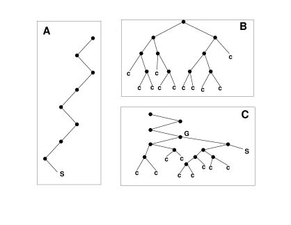
Figure 1: Types of search trees generated by the DPLL solving procedure for variables taking $v=2$ values at most. Nodes (black dots) stand for the choices of variables made by the heuristic, and edges between nodes denote the elimination of unitary clauses. A. simple branch: the algorithm finds easily a solution without ever backtracking. B. dense tree: in the absence of solution, the algorithm builds a “bushy” tree, with many branches of various lengths, before stopping. C. mixed case, branch + tree: if many contradictions arise before reaching a solution, the resulting search tree can be decomposed in a single branch followed by a dense tree. The junction G is the highest backtracking node reached back by DPLL.

A computer independent measure of computational complexity, that is, the amount of operations necessary to solve the instance, is given by the size $Q$ of the search tree i.e. the number of nodes it contains. Performances can be improved by designing sophisticated heuristic rules for choosing variables (point 1). The resolution time (or complexity) is a stochastic variable depending on the instance under consideration and on the choices done by the variable assignment procedure. Its average value, $\bar{Q}$, is a function of the input distribution parameters $\pi$ e.g. the ratio $\alpha$ of clauses per variable for SAT, or the average degree $c$ for the VC of random graphs, which can be measured experimentally and that we want to calculate theoretically. More precisely, our aim is to determine the values of the input parameters for which the complexity is linear, $\bar{Q}=\gamma\,N$ or exponential, $\bar{Q}=2^{N\,\omega}$, in the size $N$ of the instance and to calculate the coefficients $\gamma,\omega$ as functions of $\pi$.

The DPLL algorithm gives rise to a dynamical process. Indeed, the initial instance is modified during the search through the assignment of some variables and the simplification of the constraints that contain these variables. Therefore, the parameters of the input distribution are modified as the algorithm runs. This dynamical process has been rigorously studied and understood in the case of a search tree reducing to one branch (tree A in Figure 1)fra2 ; Fra ; Achl ; Fri ; Kir ; kir2 . Study of trees with massive backtracking e.g. trees B and C in Fig. 1 is much more difficult. Backtracking introduces strong correlations between nodes visited by DPLL at very different times, but close in the tree. In addition, the process is non Markovian since instances attached to each node are memorized to allow the search to resume after a backtracking step.

The study of the operation of DPLL is based on the following, elementary observation. Since instances are modified when treated by DPLL, description of their statistical properties generally requires additional parameters with respects to the defining parameters $\pi$ of the input distribution. Our task therefore consists in

1. identifying these extra parameters $\pi^{\prime}$kir2 ;

2. deriving the phase diagram of this new, extended distribution $\pi,\pi^{\prime}$ to identify, in the $\pi,\pi^{\prime}$ space, the critical surface separating instances having solution with high probability (satisfiable phase) from instances having generally no solution (unsatisfiable phase), see Fig. 2.

3. tracking the evolution of an instance under resolution with time $t$ (number of steps of the algorithm), that is, the trajectory of its characteristic parameters $\pi(t),\pi^{\prime}(t)$ in the phase diagram.

Whether this trajectory remains confined to one of the two phases or crosses the boundary inbetween has dramatic consequences on the resolution complexity. We find three average behaviours, schematized on Fig. 2:

• if the initial instance has a solution and the trajectory remains in the sat phase, resolution is typically linear, and almost no backtracking is present (Fig. 1A). The coordinates of the trajectory $\pi(t),\pi^{\prime}(t)$ of the instance in the course of the resolution obey a set of coupled ordinary differential equations accounting for the changes in the distribution parameters done by DPLL.

• if the initial instance has no solution, solving the instance, that is, finding a proof of unsatisfiability, takes exponentially large time and makes use of massive backtracking (Fig. 1B). Analysis of the search tree is much more complicated than in the linear regime, and requires a partial differential equation that gives information on the population of branches with parameters $\pi,\pi^{\prime}$ throughout the growth of the search tree.

• in some intermediary regime, instances have solutions but finding one requires an exponentially large time (Fig. 1C). This may be related to the crossing of the boundary between sat and unsat phases of the instance trajectory. We have therefore a mixed behaviour which can be understood through combination of the two above cases.

We now explain how to apply concretly this approach to the cases of random SAT and VC.

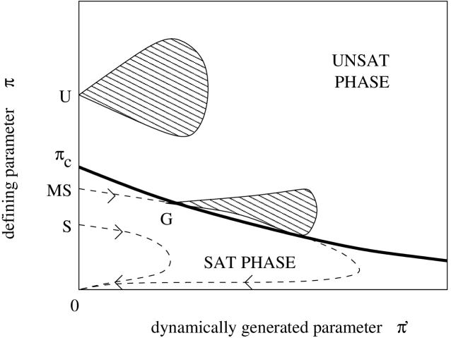
Figure 2: Schematic representation of the resolution trajectories in the sat (branch trajectories symbolized by dashed lines) and unsat (tree trajectories represented by hatched regions) phases. For simplicity we have considered the case where both $\pi$ and $\pi^{\prime}$ are scalar and not vectorial parameters. Vertical axis is the instance distribution defining parameter $\pi$. Instances are almost always satisfiable if $\pi<\pi_{c}$, unsatisfiable if $\pi>\pi_{c}$. Under the action of DPLL, the distribution of instances is modified and requires another parameter $\pi^{\prime}$ to be characterized (horizontal axis), equal to, say, zero prior to any action of DPLL. For non zero values of $\pi^{\prime}$, the critical value of the defining parameter $\pi$ obviously changes; the line $\pi_{c}(\pi^{\prime})$ defines a boundary separating typically sat from unsat instances (bold line). When the instance is unsat (point U), DPLL takes an exponential time to go through the tree trajectory. For satisfiable and easy instances, DPLL goes along a branch trajectory in a linear time (point S). The mixed case of hard sat instances (point MS) correspond to the branch trajectory crossing the boundary separating the two phases (bold line), which leads to the exploration of unsat subtrees before a solution is finally found.

II.2 Average analysis of the Random SAT problem

Figure 3: Example of 3–SAT instance and Davis-Putnam- Loveland-Logemann resolution. Step 0. The instance consists of $M=5$ clauses involving $N=4$ variables $x,y,w,z$, which can be assigned to true (T) or false (F). $\bar{w}$ means (NOT $w$) and $\vee$ denotes the logical OR. The search tree is empty. 1. DPLL randomly selects a clause among the shortest ones, and assigns a variable in the clause to satisfy it, e.g. $w=$T (splitting with the Generalized Unit Clause –GUC– heuristic fra2 ). A node and an edge symbolizing respectively the variable chosen ($w$) and its value (T) are added to the tree. 2. The logical implications of the last choice are extracted: clauses containing $w$ are satisfied and eliminated, clauses including $\bar{w}$ are simplified and the remaining ones are left unchanged. If no unitary clause (i.e. with a single variable) is present, a new choice of variable has to be made. 3. Splitting takes over. Another node and another edge are added to the tree. 4. Same as step 2 but now unitary clauses are present. The variables they contain have to be fixed accordingly. 5. The propagation of the unitary clauses results in a contradiction. The current branch dies out and gets marked with C. 6. DPLL backtracks to the last split variable ($x$), inverts it (F) and creates a new edge. 7. Same as step 4. 8. The propagation of the unitary clauses eliminates all the clauses. A solution S is found and the instance is satisfiable. For an unsatisfiable instance, unsatisfiability is proven when backtracking (see step 6) is not possible anymore since all split variables have already been inverted. In this case, all the nodes in the final search tree have two descendent edges and all branches terminate by a contradiction C.

Figure 4: Phase diagram of 2+p-SAT and resolution trajectories under DPLL action. The threshold line $\alpha_{C}(p)$ (bold full line) separates sat (lower part of the plane) from unsat (upper part) phases. Departure points for DPLL trajectories are located on the 3-SAT vertical axis. Arrows indicate the direction of ”motion” along trajectories (dashed curves) parameterized by the fraction $t$ of variables set by DPLL. For small ratios $\alpha<\alpha_{L}$ ($\simeq 3.003$ for the GUC heuristic), branch trajectories remain confined to the sat phase, end in $S$ of coordinates $(1,0)$, where a solution is found (with a search process reported on Fig. 1A). For $\alpha>\alpha_{C}\simeq 4.3$, proofs of unsatisfiability are given by complete search trees with all leaves carrying contradictions (Fig. 1B). The corresponding tree trajectories are represented by bold dashed lines (full arrows), which end up on the halting (dot-dashed) line, see text. For ratios $\alpha_{L}<\alpha<\alpha_{C}$, the branch trajectory intersects the threshold line at some point $G$. A contradiction a.s. arises, and extensive backtracking up to $G$ permits to find a solution (Fig. 1C). With exponentially small probability, the search tree looks like Fig. 1A instead: the trajectory (dashed curve) crosses the ”dangerous” region where contradictions are likely to occur, then exits from this region and ends up with a solution (lowest dashed trajectory). Inset: Resolution time of 3-SAT instances as a function of the ratio of clauses per variable $\alpha$ and for three different sizes. Data correspond to the median resolution time of 10,000 instances by DPLL; the average time may be somewhat larger due to the presence of rare, exceptionally hard instances, cf. Sec. II.4. The computational complexity is linear for $\alpha<\alpha_{L}\simeq 3.003$, exponential above.

The input distribution of 3-SAT is characterized by a single parameter $\pi$, the ratio $\alpha$ of clauses per variable. The action of DPLL on an instance of 3-SAT, illustrated in Fig. 3, causes the changes of the overall numbers of variables and clauses, and thus of $\alpha$. Furthermore, DPLL reduces some 3-clauses to 2-clauses. We use a mixed 2+p-SAT distributionSta , where $p(=\pi^{\prime})$ is the fraction of 3-clauses, to model what remains of the input instance at a node of the search tree. Using experiments and methods from statistical mechanicsSta and rigorous calculationsAchl1 , the threshold line $\alpha_{C}(p)$, separating sat from unsat phases, may be estimated with the results shown in Fig. 4. For $p\leq p_{0}=2/5$, i.e. left to point T, the threshold line is given by $\alpha_{C}(p)=1/(1-p)$, and saturates the upper bound for the satisfaction of 2-clauses. Above $p_{0}$, no exact value for $\alpha_{C}(p)$ is known. The phase diagram of 2+p-SAT is the natural space in which the DPLL dynamics takes place. An input 3-SAT instance with ratio $\alpha$ shows up on the right vertical boundary of Fig. 4 as a point of coordinates $(p=1,\alpha)$. Under the action of DPLL, the representative point moves aside from the 3-SAT axis and follows a trajectory in the $(p,\alpha)$ plane.

In this section, we show that the location of this trajectory in the phase diagram allows a precise understanding of the search tree structure and of complexity as a function of the ratio $\alpha$ of the instance to be solved (Inset of Fig. 4). In addition, we shall present an approximate calculation of trajectories accounting for the case of massive backtracking, that is for unsat instances, and slightly below the threshold in the sat phase. Our approach is based on a non rigorous extension of works by Chao and Franco who first studied the action of DPLL (without backtracking) on easy, sat instancesfra2 ; Fra as a way to obtain lower bounds to the threshold $\alpha_{C}$, see Achl for a recent review.

Let us emphasize that the idea of trajectory is made possible thanks to an important statistical property of the heuristics of split we consider fra2 ; Fra ,

• Unit-Clause (UC) heuristic: pick up randomly a literal among a unit clause if any, or any unset variable otherwise.

• Generalized Unit-Clause (GUC) heuristic: pick up randomly a literal among the shortest avalaible clauses.

• Short Clause With Majority (SC₁) heuristic: pick up randomly a literal among unit clauses if any, or pick up randomly an unset variable $v$, count the numbers of occurences $\ell,\bar{\ell}$ of $v$, $\bar{v}$ in 3-clauses, and choose $v$ (respectively $\bar{v}$) if $\ell>\bar{\ell}$ (resp. $\ell<\bar{\ell}$). When $\ell=\bar{\ell}$, $v$ and $\bar{v}$ are equally likely to be chosen.

These heuristics do not induce any bias nor correlation in the instances distributionfra2 ; kir2 . Such a statistical “invariance” is required to ensure that the dynamical evolution generated by DPLL remains confined to the phase diagram of Fig. 4. In the following, the initial ratio of clauses per variable of the instance to be solved will be denoted by $\alpha_{0}$.

II.2.1 Lower sat phase and branch trajectories.

Let us consider the first descent of the algorithm, that is the action of DPLL in the absence of backtracking. The search tree is a single branch (Fig. 1A). The numbers of 2 and 3-clauses are initially equal to $C_{2}=0,C_{3}=\alpha_{0}\,N$ respectively. Under the action of DPLL, $C_{2}$ and $C_{3}$ follow a Markovian stochastic evolution process, as the depth $T$ along the branch (number of assigned variables) increases. Both $C_{2}$ and $C_{3}$ are concentrated around their average values, the densities $c_{j}(t)=E[C_{j}(tN)/N]$ ($j=2,3$) of which obey a set of coupled ordinary differential equations (ODE)fra2 ; Fra ; Achl ,

$$\frac{dc_{3}}{dt}=-\frac{3\,c_{3}}{1-t}\qquad,\qquad\frac{dc_{2}}{dt}=\frac{3\,c_{3}}{2(1-t)}-\frac{2\,c_{2}}{1-t}-\rho_{1}(t)\;h(t)\qquad,$$ (1)

where $\rho_{1}(t)=1-c_{2}(t)/(1-t)$ is the probability that DPLL fixes a variable at depth $t$ through unit-propagation. Function $h$ depends upon the heuristic: $h_{UC}(t)=0$, $h_{GUC}(t)=1$ (if $\alpha_{0}>2/3$), $h_{SC_{1}}(t)=a\,e^{-a}\,(I_{0}(a)+I_{1}(a))/2$ with $a\equiv 3\,c_{3}(t)/(1-t)$ and $I_{\ell}$ denotes the $\ell^{th}$ modified Bessel function. To obtain the single branch trajectory in the phase diagram of Fig. 4, we solve the ODEs (1) with initial conditions $c_{2}(0)=0,c_{3}(0)=\alpha_{0}$, and perform the change of variables

$$p(t)=\frac{c_{3}(t)}{c_{2}(t)+c_{3}(t)}\qquad,\qquad\alpha(t)=\frac{c_{2}(t)+c_{3}(t)}{1-t}\qquad.$$ (2)

Results are shown for the GUC heuristics and starting ratios $\alpha_{0}=2$ and 2.8 in Fig. 4. Trajectories, indicated by light dashed lines, first head to the left and then reverse to the right until reaching a point on the 3-SAT axis at a small ratio. Further action of DPLL leads to a rapid elimination of the remaining clauses and the trajectory ends up at the right lower corner S, where a solution is found.

Frieze and Suen Fri have shown that, for ratios $\alpha_{0}<\alpha_{L}\simeq 3.003$ (for the GUC heuristics), the full search tree essentially reduces to a single branch, and is thus entirely described by the ODEs (1). The number of backtrackings necessary to reach a solution is bounded from above by a power of $\log N$. The average size $\bar{Q}$ of the branch then scales linearly with $N$ with a multiplicative factor $\gamma(\alpha_{0})=Q/N$ that can be analytically computed Coc .

The boundary $\alpha_{L}$ of this easy sat region can be defined as the largest initial ratio $\alpha_{0}$ such that the branch trajectory $p(t),\alpha(t)$ issued from $\alpha_{0}$ never leaves the sat phase in the course of DPLL resolution.

II.2.2 Unsat phase and tree trajectories.

For ratios above threshold ($\alpha_{0}>\alpha_{C}\simeq 4.3$), instances almost never have a solution but a considerable amount of backtracking is necessary before proving that clauses are incompatible. As shown in Fig. 1B, a generic unsat tree includes many branches. The number of branches (leaves), $B$, or the number of nodes, $Q=B-1$, grow exponentially with $N$Chv . It is convenient to define its logarithm $\omega$ through $B=2^{N\omega}$. Contrary to the previous section, the sequence of points $(p,\alpha)$ characterizing the evolution of the 2+p-SAT instance solved by DPLL does not define a line any longer, but rather a patch, or cloud of points with a finite extension in the phase diagram of Fig. 2.

We have analytically computed the logarithm $\omega$ of the size of these patches, as a function of $\alpha_{0}$, extending to the unsat region the probabilistic analysis of DPLL. This is, a priori, a very difficult task since the search tree of Fig. 1B is the output of a complex, sequential process: nodes and edges are added by DPLL through successive descents and backtrackings. We have imagined a different building up, that results in the same complete tree but can be mathematically analyzed: the tree grows in parallel, layer after layer (Fig. 5).

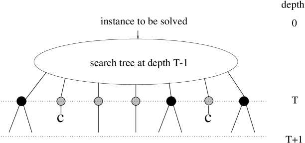
Figure 5: Imaginary, parallel growth process of an unsat search tree used in the theoretical analysis of the computational complexity. Variables are fixed through unit-propagation, or the splitting heuristics as in the DPLL procedure, but branches evolve in parallel. $T$ denotes the depth in the tree, that is the number of variables assigned by DPLL along each (living) branch. At depth $T$, one literal is chosen on each branch among 1-clauses (unit-propagation, grey circles not represented on Figure 1), or 2,3-clauses (split, black circles as in Figure 1). If a contradiction occurs as a result of unit-propagation, the branch gets marked with C and dies out. The growth of the tree proceeds until all branches carry C leaves. The resulting tree is identical to the one built through the usual, sequential operation of DPLL.

A new layer is added by assigning, according to DPLL heuristic, one more variable along each living branch. As a result, a branch may split (case 1), keep growing (case 2) or carry a contradiction and die out (case 3). Cases 1,2 and 3 are stochastic events, the probabilities of which depend on the characteristic parameters $c_{2},c_{3},t$ defining the 2+p-SAT instance carried by the branch, and on the depth (fraction of assigned variables) $t$ in the tree. We have taken into account the correlations between the parameters $c_{2},c_{3}$ on each of the two branches issued from splitting (case 1), but have neglected any further correlation which appear between different branches at different levels in the treeCoc . This Markovian approximation permits to write an evolution equation for the logarithm $\omega(c_{2},c_{3},t)$ of the average number of branches with parameters $c_{2},c_{3}$ as the depth $t$ increases,

$$\frac{\partial\omega}{\partial t}(c_{2},c_{3},t)={H}\left[c_{2},c_{3},\frac{\partial\omega}{\partial c_{2}},\frac{\partial\omega}{\partial c_{3}},t\right]\qquad.$$ (3)

${H}$ incorporates the details of the splitting heuristics. In terms of the partial derivatives $y_{2}=\partial\omega/\partial c_{2}$, $y_{3}=\partial\omega/\partial c_{3}$, we have for the UC and GUC heuristics

$${H}_{UC} = 1+\frac{1}{\ln 2}\left[\frac{3\,c_{3}}{1-t}\;\left(e^{y_{3}}\frac{1+e^{-y_{2}}}{2}-1\right)+\frac{c_{2}}{1-t}\;\left(\frac{3}{2}e^{-y_{2}}-2\right)\right]$$

$${H}_{GUC} = \log_{2}\nu(y_{2})+\frac{1}{\ln 2}\left[\frac{3\,c_{3}}{1-t}\;\left(e^{y_{3}}\frac{1+e^{-y_{2}}}{2}-1\right)+\frac{c_{2}}{1-t}\;\left(\nu(y_{2})-2\right)\right]$$

where $$\nu(y_{2})=\frac{1}{2}\;e^{y_{2}}\left(1+\sqrt{1+4e^{-y_{2}}}\right)\qquad.$$ (4)

Partial differential equation (PDE) (3) is analogous to growth processes encountered in statistical physics Gro . The surface $\omega$, growing with “time” $t$ above the plane $(c_{2},c_{3})$, or equivalently from (2), above the plane $(p,\alpha)$ (Fig. 6), describes the whole distribution of branches. The average number of branches at depth $t$ in the tree equals $B(t)=\int dp\;d\alpha\;2^{N\,\omega(p,\alpha,t)}\simeq 2^{N\,\omega^{*}(t)}$, where $\omega^{*}(t)$ is the maximum over $p,\alpha$ of $\omega(p,\alpha,t)$ reached in $p^{*}(t),\alpha^{*}(t)$. In other words, the exponentially dominant contribution to $B(t)$ comes from branches carrying 2+p-SAT instances with parameters $p^{*}(t),\alpha^{*}(t)$, which define the tree trajectories on Fig. 4.

The hyperbolic line in Fig. 4 indicates the halt points, where contradictions prevent dominant branches from further growing. Each time DPLL assigns a variable through unit-propagation, an average number $u(p,\alpha)$ of new 1-clauses is produced, resulting in a net rate of $u-1$ additional 1-clauses. As long as $u<1$, 1-clauses are quickly eliminated and do not accumulate. Conversely, if $u>1$, 1-clauses tend to accumulate. Opposite 1-clauses $x$ and $\bar{x}$ are likely to appear, leading to a contradiction Fra ; Fri . The halt line is defined through $u(p,\alpha)=1$. As far as dominant branches are concerned, the equation of the halt line reads

$$\alpha=\left(\frac{3+\sqrt{5}}{2}\right)\ln\left[\frac{1+\sqrt{5}}{2}\right]\;\frac{1}{1-p}\simeq\frac{1.256}{1-p}\qquad.$$ (5)

Along the tree trajectory, $\omega^{*}(t)$ grows from 0, on the right vertical axis, up to some final positive value, $\hat{\omega}$, on the halt line. $\hat{\omega}$ is our theoretical prediction for the logarithm of the complexity (divided by $N$). Values of $\hat{\omega}$ obtained for $4.3<\alpha_{0}<20$ by solving equation (3) compare very well with numerical results Coc .

Figure 6: Snapshots of the surface $\omega(p,\alpha)$ for $\alpha_{0}=10$ at three different depths, $t=0.01$, 0.05 and 0.09 (from left to right). The height $\omega^{*}(t)$ of the top of the surface, with coordinates $p^{*}(t),\alpha^{*}(t)$, is the logarithm (divided by $N$) of the number of branches. The halt line is hit at $t_{h}\simeq 0.094$.

We have plotted the surface $\omega$ above the $(p,\alpha)$ plane, with the results shown in Fig. 6. It must be stressed that, though our calculation is not rigorous, it provides a very good quantitative estimate of the complexity. Furthermore, complexity is found to scale asymptotically as

$$\hat{\omega}(\alpha_{0})\sim\frac{3+\sqrt{5}}{(6\,\ln 2)\;\alpha_{0}}\;\left[\ln\left(\frac{1+\sqrt{5}}{2}\right)\right]^{2}\simeq\frac{0.292}{\alpha_{0}}\qquad(\alpha_{0}\gg\alpha_{C}).$$ (6)

This result exhibits the expected scalingBea , and could indeed be exact. As $\alpha_{0}$ increases, search trees become smaller and smaller, and correlations between branches, weaker and weaker.

II.2.3 Upper sat phase and mixed branch–tree trajectories.

The interest of the trajectory approach proposed in this paper is best seen in the upper sat phase, that is ratios $\alpha_{0}$ ranging from $\alpha_{L}$ to $\alpha_{C}$. This intermediate region juxtaposes branch and tree behaviors, see Fig. 1C. The branch trajectory starts from the point $(p=1,\alpha_{0})$ corresponding to the initial 3-SAT instance and hits the critical line $\alpha_{c}(p)$ at some point G with coordinates ($p_{G},\alpha_{G}$) after $N\;t_{G}$ variables have been assigned by DPLL (Fig. 4). The algorithm then enters the unsat phase and generates 2+p-SAT instances with no solution. A dense subtree, that DPLL has to go through entirely, forms beyond G till the halt line (Fig. 4). The size of this subtree, $2^{N\,(1-t_{G})\,\hat{\omega}_{G}}$, can be analytically predicted from our theory. G is the highest backtracking node in the tree (Fig. 1C) reached back by DPLL, since nodes above G are located in the sat phase and carry 2+p-SAT instances with solutions. DPLL will eventually reach a solution. The corresponding branch (rightmost path in Fig. 1C) is highly non typical and does not contribute to the complexity, since almost all branches in the search tree are described by the tree trajectory issued from G (Fig. 4). We have checked experimentally this scenario for $\alpha_{0}=3.5$. The coordinates of the average highest backtracking node, $(p_{G}\simeq 0.78,\alpha_{G}\simeq 3.02$), coincide with the analytically computed intersection of the single branch trajectory and the critical line $\alpha_{c}(p)$Coc . As for complexity, experimental measures of $\omega$ from 3-SAT instances at $\alpha_{0}=3.5$, and of $\omega_{G}$ from 2+0.78-SAT instances at $\alpha_{G}=3.02$, obey the expected identity $\omega=\omega_{G}\;(1-t_{G})$ and are in very good agreement with theoryCoc . Therefore, the structure of search trees for 3-SAT reflects the existence of a critical line for 2+p-SAT instances.

II.3 Average analysis of the vertex cover of random graphs

We now consider the VC problem, where inputs are random graphs drawn from the $G(N,p=c/N)$ ensembleBollo . In other words, graphs have $N$ vertices and the probability that a pair of vertices are linked through an edge is $c/N$, independently of other edges. When the number $X=xN$ of covering marks is lowered, the model undergoes a COV/UNCOV transition at some critical density of covers $x_{\rm c}(c)$ for $N\to\infty$. For $x>x_{\rm c}(c)$, vertex covers of size $Nx$ exist with probability one, for $x<x_{\rm c}(c)$ the available covering marks are not sufficient. The statistical mechanics analysis of Ref. WeHa1 gave the result

$$x_{\rm c}(c)=1-\frac{2W(c)+W(c)^{2}}{2c}\,,\;\;\;\;\;\;\;\;\mbox{for}\;\;c<e\,,$$ (7)

where $W(c)$ solves the equation $We^{W}=c$. This result is compatible with the bounds of Refs. Ga_VC ; Fr_VC , and was later shown to be exact Bauer . For $c>e$, Eq. (7) only gives an approximate estimate of $x_{\rm c}(c)$. More sophisticated calculations can be found in Ref. WeHaLong .

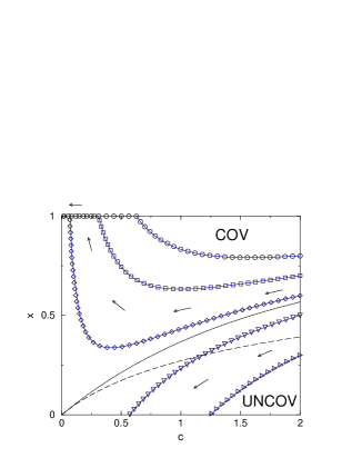
Figure 7: Phase diagram of VC. The low-$x$, high-$c$ UNCOV phase is separated by the dashed line, cf. Eq. (7), from the high-$x$, low-$c$ COV phase. The symbols (numerics) and continuous lines (analytical prediction, cf. Eq. (8)) refer to the simple search algorithm described in the text. The dotted line is the separatrix between two types of trajectories.

Let us consider a simple implementation of the DPLL procedure for the present problem. During the computation, vertices can be covered, uncovered or just free, meaning that the algorithm has not yet assigned any value to that vertex. At the beginning all the vertices are set free. At each step the algorithm chooses a vertex $i$ at random among those which are free. If $i$ has neighboring vertices which are either free or uncovered, then the vertex $i$ is declared covered first. In case $i$ has only covered neighbors, the vertex is declared uncovered. The process continues unless the number of covered vertices exceeds $X$. In this case the algorithm backtracks and the opposite choice is taken for the vertex $i$ unless this corresponds to declaring uncovered a vertex that has one or more uncovered neighbors. The algorithm halts if it finds a solution (and declares the graph to be COV) or after exploring all the search tree (in this case it declares the graph to be UNCOV).

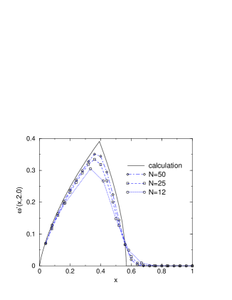
Figure 8: Number of operations required to solve (or to show that no solution exists to) the VC decision problem with the search algorithm described in the text. The logarithm of the number of nodes of the backtracking tree divided by the size $N$, is plotted versus the number of covering marks. Here we consider random instances with average connectivity $c=2$. The phase transition is at $x_{\rm c}(c=2)\approx 0.3919$ and corresponds to the peak in computational complexity.

Of course one can improve over this algorithm by using smarter heuristics WeHeur . One remarkable example is the “leaf-removal” algorithm defined in Ref. Bauer . Instead of picking any vertex randomly, one chooses a connectivity-one vertex, declare it uncovered, and declare covered its neighbor. This procedure is repeated iteratively on the subgraph of free nodes, until no connectivity-one nodes are left. In the low-connectivity, COV region $\{c<e,x>x_{\rm c}(c)\}$, it stops only when the graph is completely covered. As a consequence, this algorithm can solve VC in linear time with high probability in all this region. No equally good heuristics exists for higher connectivity, $c>e$.

II.3.1 Branch trajectories

Under the action of one of the above algorithms, the instance is progressively modified and the number of variables is reduced. In fact, at each step a vertex is selected and can be eliminated from the graph regardless whether it is declared covered or uncovered. The analysis of the first algorithm is greatly simplified by the remark that, as long as backtracking has not begun, the new vertex is selected randomly. This implies that the modified instance produced by the algorithm is still a random graph. Its evolution can be effectively described by a trajectory in the $(c,x)$ space. If one starts from the parameters $c_{0}$, $x_{0}$, after $Nt$ steps of the algorithm, he will end up with a new instance of size $N(1-t)$ and parameters WeHa2

$$c(t)=c_{0}(1-t)\,,\;\;\;\;\;x(t)=\frac{x_{0}-t}{1-t}+\frac{e^{-c_{0}(1-t)}-e^{-c_{0}}}{c_{0}(1-t)}\,.$$ (8)

Some examples of the two types of trajectories (the ones leading to a solution and the ones which eventually enter the UNCOV region) are shown in Fig. 7. The separatrix is given by

$$x_{\rm s}(c)=1-\frac{1-e^{-c}}{c}\,,$$ (9)

and corresponds to the dotted line in Fig. 7. Above this line the algorithm solves the problem in linear time.

For more general heuristics the analysis becomes less straightforward because the graph produced by the algorithm does not belong to the standard random-graph ensemble. It may be necessary to augment the number of parameters which describe the evolution of the instance. As an example, the leaf-removal algorithm mentioned in the previous Section is conveniently described by keeping track of three numbers which parametrize the degree profile (i.e. the fraction of vertices $p_{d}(t)$ having a given degree $d$) of the graph WeHeur .

II.3.2 Tree trajectories

Below the critical line $x_{\rm c}(c)$, cf. Eq. (7), no solution exists to the typical random instance of VC. Our algorithm must explore a large backtracking tree to prove it and this takes an exponential time. The size of the backtracking tree could be computed along the lines of Sec. II.B.2. However a good result can be obtained with a simple “static” calculation WeHa1 .

As explained in Sec. II.B.2, we imagine the evolution of the backtracking tree as proceeding “in parallel”. At the level $M$ of the tree a set of $M$ vertices has been visited. Call ${\cal G}_{M}$ the subgraph induced by these vertices. Since we always put a covering mark on a vertex which is surrounded by vertices declared uncovered, each node of the backtracking tree will carry a vertex cover of the associated subgraph ${\cal G}_{M}$ . Therefore the number of backtracking nodes is given by

$$Q=\sum_{M=1}^{N}{\cal N}_{\rm VC}({\cal G}_{M};X)\,,$$ (10)

where ${\cal N}_{\rm VC}({\cal G}_{M};X)$ is the number of VC’s of ${\cal G}_{M}$ using at most $X$ marks. A very crude estimate of the right-hand side of the above equation is:

$$Q\leq\sum_{M=1}^{N}\sum_{X^{\prime}=0}^{{\rm min}(X,M)}\left(\begin{array}[]{c}M\\ X^{\prime}\end{array}\right)\,,$$ (13)

where we bounded the number of VC’s of size $X^{\prime}$ on ${\cal G}_{M}$ with the number of ways of placing $X^{\prime}$ marks on $M$ vertices. The authors of WeHa2 provided a refined estimate based on the annealed approximation of statistical mechanics. The results of this calculation are compared in Fig. 8 with the numerics.

II.3.3 Mixed trajectories

If the parameters which characterize an instance of VC lie in the region between $x_{\rm c}(c)$, cf. Eq. (7), and $x_{\rm s}(c)$, cf. Eq. (9), the problem is still soluble but our algorithm takes an exponential time to solve it. In practice, after a certain number of vertices has been visited and declared either covered or uncovered, the remaining subgraph ${\cal G}_{free}$ cannot be any longer covered with the leftover marks. This happens typically when the first descent trajectory (8) crosses the critical line (7).

It takes some time for the algorithm to realize this fact. More precisely, it takes exactly the time necessary to prove that ${\cal G}_{free}$ is uncoverable. This time dominates the computational complexity in this region and can be calculated along the lines sketched in the previous Section. The result is, once again, reported in Fig. 8, which clearly shows a computational peak at the phase boundary.

Finally, let us notice that this mixed behavior disappears in the entire $c<e$ region if the leaf-removal heuristics is adopted for the first descent.

II.4 Distribution of resolution times

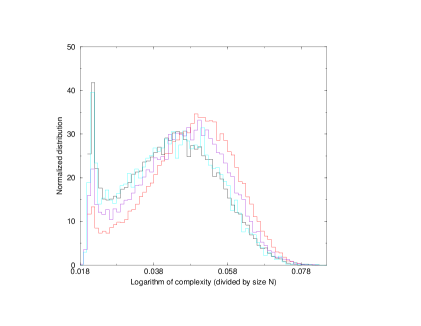
Figure 9: Probability distributions of the logarithm $\omega$ of the resolution complexity from 20,000 runs of DPLL on random 3-SAT instances with ratio $\alpha=3.5$. Each distribution corresponds to one randomly drawn instance of size $N=300$.

Figure 10: Resolution of random 3-SAT instances in the upper sat phase: logarithm of complexity with DPLL ($\omega$ – simulations: circles, theory: dotted line) and restarts ($\zeta$ – simulations: squares, theory: full line) as a function of ratio $\alpha$. Inset: Minus log. of the cumulative probability $P_{lin}$ of complexities $Q\leq N$ as a function of the size for $100\leq N\leq 400$ (full line); log. of the number of restarts $N_{rest}$ necessary to find a solution for $100\leq N\leq 1000$ (dotted line) for $\alpha=3.5$. Slopes are $\zeta=0.0011$ and $\bar{\zeta}=0.00115$ respectively.

Up to now we have studied the typical resolution complexity. The study of fluctuations of resolution times is interesting too, particularly in the upper sat phase where solutions exist but are found at a price of a large computational effort. We may expect that there exist lucky but rare resolutions able to find a solution in a time much smaller than the typical one. Due to the stochastic character of DPLL complexity indeed fluctuates from run to run of the algorithm on the same instance. In Fig. 9 we show this run-to-run distribution of the logarithm $\omega$ of the resolution complexity for four instances of random 3-SAT with the same ratio $\alpha=3.5$. The run to run distribution are qualitatively independent of the particular instances, and exhibit two bumps. The wide right one, located in $\omega\simeq 0.035$, correspond to the major part of resolutions. It acquires more and more weight as $N$ increases and corresponds to the typical behavior analysed in Section II.B.3. The left peak corresponds to much faster resolutions, taking place in linear time. The weight of this peak (fraction of runs with complexities falling in the peak) decreases exponentially fast with $N$, and can be numerically estimated to $W_{lin}=2^{-N\zeta}$ with $\zeta\simeq 0.011$. Therefore, instances at $\alpha=3.5$ are typically solved in exponential time but a tiny (exponentially small) fraction of runs are able to find a solution in linear time only.

A systematic stop-and-restart procedure may be introduced to take advantage of this fluctuation phenomenon and speed up resolution. If a solution is not found before $N$ splits, DPLL is stopped and rerun after some random permutations of the variables and clauses. The expected number $N_{rest}$ of restarts necessary to find a solution being equal to the inverse probability $1/W_{lin}$ of linear resolutions, the resulting complexity scales as $N\;W_{lin}^{-1}\sim 2^{N\,\zeta}$.

To calculate $\zeta$ we have analyzed, along the lines of the study of the growth of the search tree in the unsat phase, the whole distribution of the complexity for a given ratio $\alpha$ in the upper sat phase. Calculations can be found in Cocrs . Linear resolutions are found to correspond to branch trajectories that cross the unsat phase without being hit by a contradiction, see Fig. 4. Results are reported in Fig. 10 and compare very well with the experimentally measured number $N_{rest}$ of restarts necessary to find a solution. In the whole upper sat phase, the use of restarts offers an exponential gain with respect to usual DPLL resolution (see Fig. 10 for comparison between $\zeta$ and $\omega$), but the completeness of DPLL is lost.

Figure 11: The computational complexity of the search algorithm for VC, with restarts after $\exp(N\omega^{\prime}_{R})$ backtracking steps. The complexity is defined as the logarithm of the total number of visited nodes, divided by the size $N$ of the graph. Symbols refer to $N=30$ (circles), $60$ (triangles), and $120$ (diamonds). The stars are the result of an $N\to\infty$ extrapolation. The continuous (dashed) line reproduces the theoretical prediction with (without) taking into account fluctuations of the first descent trajectory.

A slightly more general restart strategy consists in stopping the backtracking procedure after a fixed number of nodes $Q_{R}=e^{N\omega^{\prime}_{R}}$ has been visited. A new (and statistically independent) DPLL procedure is then started from the beginning. In this case one exploits lucky, but still exponential, stochastic runs. The tradeoff between the exponential gain of time and the exponential number of restarts, can be optimized by tuning the parameter $\omega^{\prime}_{R}$. This approach has been analyzed in Ref. VCRestart taking VC as a working example. In Fig. 11 we show the computatonal complexity of such a strategy as a function of the restart parameter $\omega^{\prime}_{R}$. We compare the numerics with an approximate calculation VCRestart . The instances were random graphs with average connectivity $c=3.2$, and $x=0.6$ covering marks per vertex. The optimal choice of the parameter seems to be (in this case) $\omega^{\prime}_{R}\approx 0$, corresponding to polynomial runs.

Figure 12: Restart experiments for VC with initial condition at $c_{0}=3.2$, $x_{0}=0.6$ (empty circle). The long-dashed line is the critical line (7). The rightmost dotted line is the typical trajectory. The leftmost one is the rare trajectory followed by the last (successful) restart of the algorithm when $\omega^{\prime}_{R}=0.1$. The symbols are numerical results for the $(c,x)$ coordinates of the root of the backtrack tree generated by the algorithm since the last restart. Triangles, squares and stars correspond, respectively, to $N=30$, $60$, $120$ (in each case we considered several values for $\omega^{\prime}_{R}$, each one corresponding to a symbol). The continuous line is an approximate analytical prediction for the same quantity.

The analytical prediction reported in Fig. 11 requires, as for 3-SAT, an estimate of the execution-time fluctuations of the DPLL procedure (without restart). It turns out that one major source of fluctuations is, in the present case, the location in the $(c,x)$ plane of the highest node in the backtracking tree. In the typical run this coincides with the intersection $(c_{G},x_{G})$ between the first descent trajectory (8) and the critical line (7). One can estimate the probability $P(c,x)\sim\exp\{-N\psi(c,x)\}$ for this node to have coordinates $(c,x)$ (obviously $\psi(c_{G},x_{G})=0$).

When an upper bound $\omega^{\prime}_{R}$ on the backtracking time is fixed, the problem is solved in those lucky runs which are characterized by an atypical highest backtracking node. Roughly speaking, this means that the algorithm has made some very good (random) choices in its first steps. In Fig. 12 we plot the position of the highest backtracking point in the (last) successful runs for several values of $\omega^{\prime}_{R}$. Once again the numerics compare favourably with an approximate calculation.

III Analysis of local search algorithms

We now turn to the description and study of algorithms of another type, namely local search algorithms. As a common feature, these algorithms start from a configuration (assignment) of the variables, and then make successive improvements by changing at each step few of the variables in the configuration (local move). For instance, in the SAT problem, one variable is flipped from being true to false, or vice versa, at each step. Whereas complete algorithms of the DPLL type give a definitive answer to any instance of a decision problem, exhibiting either a solution or a proof of unsatisfiability, local search algorithms give a sure answer when a solution is found but cannot prove unsatisfiability. However, these algorithms can sometimes be turned into one-sided probabilistic algorithms, with an upper bound on the probability that a solution exists and has not been found after $T$ steps of the algorithm, decreasing to zero when $T\to\infty$rando .

III.1 Landscape and search dynamics

Local search algorithms perform repeated changes of a configuration $C$ of variables (values of the Boolean variables for SAT, status –marked or unmarked– of vertices for VC) according to some criterion, usually based on the comparison of the cost function $F$ (number of unsatisfied clauses for SAT, of uncovered edges for VC) evaluated at $C$ and over its neighborhood. It is therefore clear that the shape of the multidimensional surface $C\to F(C)$, called cost function landscape, is of high importance. On intuitive grounds, if this landscape is relatively smooth with a unique minimum, local procedures as gradient descent should be very efficient, while the presence of many local minima could hinder the search process (Fig. 13). The fundamental underlying question is whether the performances of the dynamical process (ability to find the global minimum, time needed to reach it) can be understood in terms of an analysis of the cost function landscape only.

This question was intensively studied and answered for a limited class of cost functions, called mean field spin glass models, some years agoleti . The characterization of landscapes is indeed of huge importance in physical systems. There, the cost function is simply the physical energy, and local dynamics are usually low or zero temperature Monte Carlo dynamics, essentially equivalent to gradient descent. Depending on the parameters of the input distribution, the minima of the cost functions may undergo structural changes, a phenomenon called clustering in physics.

Clustering has been rigorously shown to take place in the random 3-XORSAT problemCrei ; xorsat1 ; xorsat2 , and is likely to exist in many other random combinatorial problems as 3-SATvaria ; cavi . Instances of the 3-XORSAT problem with $M=\alpha\,N$ clauses and $N$ variables have almost surely solutions as long as $\alpha<\alpha_{c}\simeq 0.918$xorsat1 ; xorsat2 . The clustering phase transition takes place at $\alpha_{s}\simeq 0.818$ and is related to a change in the geometric structure of the space of solutions, see Fig. 13:

• when $\alpha<\alpha_{s}$, the space of solutions is connected. Given a pair of solutions $C,C^{\prime}$, i.e. two assignments of the $N$ Boolean variables that satisfy the clauses, there almost surely exists a sequence of solutions, $C_{j},j=0,1,2,\ldots,J$, with $C_{0}\equiv C$, $C_{J}\equiv C^{\prime}$, $J=O(N)$, connecting the two solutions such that the Hamming distance (number of different variables) between $C_{j}$ and $C_{j+1}$ is bounded from above by some finite constant when $N\to\infty$.

• when $\alpha_{s}<\alpha<\alpha_{c}$, the space of solutions is not connected any longer. It is made of an exponential (in $N$) number of connected components, called clusters, each containing an exponentially large number of solutions. Clusters are separated by large voids: the Hamming distance between two clusters, that is, the smallest Hammming distance between pairs of solutions belonging to these clusters, is of the order of $N$.

From intuitive grounds, changes of the statistical properties of the cost function landscape e.g. of the structure of the solutions space may potentially affect the search dynamics. This connection between dynamics and static properties was established in numerous works in the context of mean field models of spin glasses leti , and subsequently also put forward in some studies of local search algorithms in combinatorial optimization problemsvaria ; suedois ; cavi . So far, there is no satisfying explanation to when and why features of a priori algorithm dependent dynamical phenomena should be related to, or predictable from some statistical properties of the cost function landscape. We shall see some examples in the following where such a connection indeed exist (Sec. III.B) and other ones where its presence is far less obvious (Sec. IIIC,D).

Figure 13: Landscapes corresponding to three different cost functions. Horizontal axis represent the space of configurations $C$, while vertical axis is the associated cost $F(C)$. Left: smooth cost function, with a single minimum easily reachable with local search procedures e.g. gradient descent. Middle: rough cost function with a lot of local minima whose presence may damage the performances of local search algorithms. The various global minima are spread out homogeneously over the configuration space. Right: rough cost function with global minima clustered in some portions of the configuration space only.

III.2 Algorithms for error correcting codes

Figure 14: Tanner graph of a regular linear code. A left-hand node is associated to each variable, and a right hand node to each parity check. A link is drawn between two nodes whenever the variable associated to the left-hand one enters in the parity check corresponding to the right-hand one.

Coding theory is a rich source of computational problems (and algorithms) for which the average case analysis is relevant Barg ; Spielman . Let us focus, for sake of concreteness, on the decoding problem. Codewords are sequences of symbols with some built-in redundancy. If we consider the case of linear codes on a binary alphabet, this redundancy can be implemented as a set of linear constraints. In practice, a codeword is a vector $\underline{{\tt x}}\in\{0,1\}^{N}$ (with $N\gg 1$) which satisfies the equation

$${\mathbb{H}}\,\underline{{\tt x}}=\underline{{\tt 0}}\;\;\;\;({\rm mod}\;\;\;2)\,,$$ (14)

where ${\mathbb{H}}$ is an $M\times N$ binary matrix (parity check matrix). Each one of the $M$ linear equations involved in Eq. (14) is called a parity check. This set of equation can be represented graphically by a Tanner graph, cf. Fig. 14. This is a bipartite graph highlighting the relations between the variables ${\tt x}_{i}$ and the constraints (parity checks) acting on them. The decoding problem consists in finding, among the solutions of Eq. (14), the “closest” one $\underline{{\tt x}}_{\rm d}$ to the output $\underline{{\tt x}}_{\rm out}$ of some communication channel. This problem is, in general, NP-hard Berlekamp .

The precise meaning of “closest” depends upon the nature of the communication channel. Let us make two examples:

• The binary symmetric channel (BSC). In this case the output of the communication channel $\underline{{\tt x}}_{\rm out}$ is a codeword, i.e. a solution of (14), in which a fraction $p$ of the entries has been flipped. “Closest” has to be understood in the Hamming-distance sense. $\underline{{\tt x}}_{\rm d}$ is the solution of Eq. (14) which minimizes the Hamming distance from $\underline{{\tt x}}_{\rm out}$.

• The binary erasure channel (BEC). The output $\underline{{\tt x}}_{\rm out}$ is a codeword in which a fraction $p$ of the entries has been erased. One has to find a solution $\underline{{\tt x}}_{\rm d}$ of Eq. (14) which is compatible with the remaining entries. Such a problem has a unique solution for small enough erasure probability $p$.

There are two sources of randomness in the decoding problem: $(i)$ the matrix ${\mathbb{H}}$ which defines the code is usually drawn from some random ensemble; $(ii)$ the received message which is distributed according to some probabilistic model of the communication channel (in the two examples above, the bits to be flipped/erased were chosen randomly). Unlike many other combinatorial problems, there is therefore a “natural” probability distribution defined on the instances. Average case analysis with respect to this distribution is of great practical relevance.

Recently, amazingly good performances have been obtained by using low-density parity check (LDPC) codes Chung . LDPC codes are defined by parity check matrices ${\mathbb{H}}$ which are large and sparse. As an example we can consider Gallager regular codes GallagerThesis . In this case ${\mathbb{H}}$ is chosen with flat probability distribution within the family of matrices having $l$ ones per column, and $k$ ones per row. These are decoded using a suboptimal linear-time algorithm known as “belief-propagation” or “sum-product” algorithm GallagerThesis ; Pearl . This is an iterative algorithm which takes advantage of the locally tree-like structure of the Tanner graph, see Fig. 14, for LDPC codes. After $n$ iterations it incorporates the information conveyed by the variables up to distance $n$ from the one to be decoded. This can be done in a recursive fashion allowing for linear-time decoding.

Belief-propagation decoding shows a striking threshold phenomenon as the noise level $p$ crosses some critical (code-dependent) value $p_{d}$. While for $p<p_{d}$ the transmitted codeword is recovered with high probability, for $p>p_{d}$ decoding will fail almost always. The threshold noise $p_{d}$ is, in general, smaller than the threshold $p_{c}$ for optimal decoding (with unbounded computational resources).

The rigorous analysis of Ref. RichardsonUrbankeIntroduction allows a precise determination of the critical noise $p_{d}$ under quite general circumstances. Nevertheless some important theoretical questions remain open: Can we find some smarter linear-time algorithm whose threshold is greater than $p_{d}$? Is there any “intrinsic” (i.e. algorithm independent) characterization of the threshold phenomenon taking place at $p_{d}$? As a first step towards the answer to these questions, Ref. DynamicCodes explored the dynamics of local optimization algorithms by using statistical mechanics techniques. The interesting point is that “belief propagation” is by no means a local search algorithm.

For sake of concreteness, we shall focus on the binary erasure channel. In this case we can treat decoding as a combinatorial optimization problem within the space of bit sequences of length $Np$ (the number of erased bits, the others being fixed by the received message). The function to be minimized is the energy density

$$\epsilon(\underline{{\tt x}})=\frac{2}{N}d_{H}({\mathbb{H}}\underline{{\tt x}},\underline{{\tt 0}})\,,$$ (15)

where we denote as $d_{H}(\underline{{\tt x}}_{1},\underline{{\tt x}}_{2})$ the Hamming distance between two vectors $\underline{{\tt x}}_{1}$ and $\underline{{\tt x}}_{2}$, and we introduced the normalizing factor for future convenience. Notice that both arguments of $d_{H}(\cdot,\cdot)$ in Eq. (15) are vectors in $\{0,1\}^{M}$.

We can define the $R$-neighborhood of a given sequence $\underline{{\tt x}}$ as the set of sequences $\underline{{\tt z}}$ such that $d_{\rm H}(\underline{{\tt x}},\underline{{\tt z}})\leq R$, and we call $R$-stable states the bit sequences which are optima of the decoding problem within their $R$-neighborhood.

Figure 15: The $(6,3)$ Gallager code decoded by local search with $1$-neighborhoods. At each time step, the algorithm looks for a bit (among the ones uncorrectly received) such that flipping it decreases the cost function (15). We plot the average number of violated parity checks (multiplied by $2/N$) after the algorithm halts, as a function of the erasure probability $p$.

One can easily invent local search algorithms papadimi for the decoding problem which use the $R$-neighborhoods. The algorithm start from a random sequence and, at each step, optimize it within its $R$-neighborhood. This algorithm is clearly suboptimal and halts on $R$-stable states. Let us consider, for instance, a $(k=6,l=3)$ regular code and decode it by local search in $1$-neighborhoods. In Fig. 15 we report the resulting energy density $\epsilon$ after the local search algorithm halts, as a function of the erasure probability $p$. We averaged over 100 different realizations of the noise and of the matrix ${\mathbb{H}}$. For sake of comparison we recall that the threshold for belief-propagation decoding is $p_{d}\approx 0.429440$ RichardsonUrbankeIntroduction , while the threshold for optimal decoding is at $p_{c}\approx 0.488151$ DynamicCodes . It is evident that local search by $1$-neighborhoods performs quite poorly.

A natural question is whether (and how much), these performances are improved by increasing $R$. It is therefore quite natural to study metastable states. These are $R$-stable states for any $R=o(N)$. There exists no completely satisfying definition of such states: here we shall just suggest a possibility among others. The tricky point is that we do not know how to compare $R$-stable states for different values of $N$. This forbids us to make use of the above asymptotic statement. One possibility is to count without really defining them. This can be done, at least in principle, by counting $R$-stable states, take the $N\to\infty$ limit and, at the end, the $R\to\infty$ limitgiu . On physical grounds, we expect $R$-stable states to be exponentially numerous. In particular, if we call ${\cal N}_{R}(\epsilon)$ the number of $R$-stable states taking a value $\epsilon$ of the cost function (15), we have

$${\cal N}_{R}(\epsilon)\sim\exp\{NS_{R}(\epsilon)\}\,.$$ (16)

We can therefore define the so called (physical) complexity $\Sigma(\epsilon)$ as follows,

$$\Sigma(\epsilon)\equiv\lim_{R\to\infty}S_{R}(\epsilon)\,.$$ (17)

Roughly speaking we can say that the number of metastable states is $\exp\{N\Sigma(\epsilon)\}$. Of course there are several alternative ways of taking the limits $R\to\infty$, $N\to\infty$, and we do not yet have a proof that these procedures give the same result for $\Sigma(\epsilon)$. Nevertheless it is quite clear that the existence of an exponential number of metastable states should affect dramatically the behavior of local search algorithms.

Figure 16: The complexity $\Sigma(\epsilon)$ of a $(6,3)$ code on the BEC, for (from top to bottom) $p=0.45$ (below $p_{c}$), $p=0.5$, and $p=0.55$ (above $p_{c}$). Recall that $\Sigma(\epsilon)$ is positive only above $p_{d}\approx 0.429440$.

Statistical mechanics methods DynamicCodes allows to determine the complexity $\Sigma(\epsilon)$ Remi . In “difficult” cases (such as for error-correcting codes), the actual computation may involve some approximation, e.g. the use of a variational Ansatz. Nevertheless the outcome is usually quite accurate. In Fig. 16 we consider a $(6,3)$ regular code on the binary erasure channel. We report the resulting complexity for three different values of the erasure probability $p$. The general picture is as follows. Below $p_{d}$ there is no metastable state, except the one corresponding to the correct codeword. Between $p_{d}$ and $p_{c}$ there is an exponential number of metastable states with energy density belonging to the interval $\epsilon_{GS}<\epsilon<\epsilon_{D}$ ($\Sigma(\epsilon)$ is strictly positive in this interval). Above $p_{c}$, $\epsilon_{GS}=0$. The maximum of $\Sigma(\epsilon)$ is always at $\epsilon_{D}$.

Figure 17: The $(6,3)$ LDPC code on the BSC decoded by simulated annealing. The circles give the number of violated checks in the resulting sequence. The continuous line is the analytical result for the typical energy density of metastable states ($\epsilon_{D}$ in Fig. 16).

The above picture tell us that any local algorithm will run into difficulties above $p_{d}$. In order to confirm this picture, the authors of Ref. DynamicCodes made some numerical computations using simulated annealing as decoding algorithm for quite large codes ($N=10^{4}$ bits). For each value of $p$, we start the simulation fixing a fraction $(1-p)$ of spins to $\sigma_{i}=+1$ (this part will be kept fixed all along the run). The remaining $pN$ spins are the dynamical variables we change during the annealing in order to try to satisfy all the parity checks. The energy of the system counts the number of unsatisfied parity checks.

The cooling schedule has been chosen in the following way: $\tau$ Monte Carlo sweeps (MCS)  at each of the 1000 equidistant temperatures between $T=1$ and $T=0$. The highest temperature is such that the system very rapidly equilibrates. Typical values for $\tau$ are from 1 to $10^{3}$.

Notice that, for any fixed cooling schedule, the computational complexity of the simulated annealing method is linear in $N$. Then we expect it to be affected by metastable states of energy $\epsilon_{D}$, which are present for $p>p_{d}$: the energy relaxation should be strongly reduced around $\epsilon_{D}$ and eventually be completely blocked. Some results are plotted in Fig. 17 together with the theoretical prediction for $\epsilon_{D}$. The good agreement confirm our picture: the algorithm gets stucked in metastable states, which have, in the great majority of cases, energy density $\epsilon_{D}$.

Both “belief propagation” and local search algorithms fail to decode correctly between $p_{d}$ and $p_{c}$. This leads naturally to the following conjecture: no linear time algorithm can decode in this regime of noise. The (typical case) computational complexity changes from being linear below $p_{d}$ to superlinear above $p_{d}$. In the case of the binary erasure channel it remains polynomial between $p_{d}$ and $p_{c}$ (since optimal decoding can be realized with linear algebra methods). However it is plausible that for a general channel it becomes non-polynomial.

III.3 Gradient descent and XORSAT

In this section the local procedure we consider is gradient descent (GD). GD is defined as follows. (1) Start from an initial randomly chosen configuration of the variables. Call $E$ the number of unsatisfied clauses. (2) If $E=0$ then stop (a solution is found). Otherwise, pick randomly one variable, say $x_{i}$, and compute the number $E^{\prime}$ of unsatisfied clauses when this variable is negated; if $E^{\prime}\geq E$ then accept this change i.e. replace $x_{i}$ with $\bar{x}_{i}$ and $E$ with $E^{\prime}$; if $E^{\prime}>E$, do not do anything. Then go to step 2. The study of the performances of GD to find the minima of cost functions related to statistical physics models has recently motivated various studiesgdphys ; gdproof . Numerics indicate that GD is typically able to solve random 3-SAT instances with ratios $\alpha<3.9$ suedois ; cavi close to the onset of clustering varia ; cavi ; par . We shall rigorously show below that this is not so for 3-XORSAT.

Let us apply GD to an instance of XORSAT. The instance has a graph representation explained in Fig. 18. Vertices are in one–to–one correspondence with variables. A clause is fully represented by a plaquette joining three variables and a Boolean label equal to the number of negated variables it contains modulo 2 (not represented on Fig. 18). Once a configuration of the variables is chosen, each plaquette may be labelled by its status, S or U, whether the associated clause is respectively satisfied or unsatisfied. A fundamental property of XORSAT is that each time a variable is changed, i.e. its value is negated, the clauses it belongs to change status too.

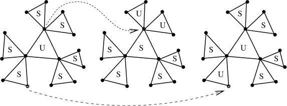
Figure 19: A blocked island (left) is an instance of 7 clauses (1 central, 6 peripherical) with variables such that the central plaquette is unsatisfied and all peripherical plaquettes are satisfied. Inversion of any variable (grey vertex) increases the number of unsatisfied clauses by 1, be it attached to the central (middle) or to a peripherical (right) plaquette.

This property makes the analysis of some properties of GD easy. Consider the hypergraph made of 15 vertices and 7 plaquettes in Fig. 19, and suppose the central plaquette is violated (U) while all other plaquettes are satisfied (S). The number of unsatisfied clauses is $E=1$. Now run GD on this special instance of XORSAT. Two cases arise, symbolized in Fig. 19, whether the vertex attached to the variable to be flipped belongs, or not, to the central plaquette. It is an easy check that, in both cases, $E^{\prime}=2$ and the change is not permitted by GD. The hypergraph of Fig. 19 will be called hereafter island. When the status of the plaquettes is U for the central one and S for the other ones, the island is called blocked. Though the instance of the XORSAT problem encoded by a blocked island is obviously satisfiable (think of negating at the same time one variable attached to a vertex $V$ of the central plaquette and one variable in each of the two peripherical plaquettes joining the central plaquette at $V$), GD will never be able to find a solution and will be blocked forever in the local minimum with height $E=1$.

The purpose of this section is to show that this situation typically happens for random instances of XORSAT. More precisely, while almost all instances of XORSAT with a ratio of clauses per variables smaller than $\alpha\simeq 0.918$ have a lot of solutions, GD is almost never able to find one. Even worse, the number of violated clauses reached by GD is bounded from below by $\Psi(\alpha)\,N$ where

$$\Psi(\alpha)=\frac{729}{1024}\,\alpha^{7}\,e^{-45\,\alpha}\qquad.$$ (18)

In other words, the number of clauses remaining unsatisfied at the end of a typical GD run is of the order of $N$. Our demonstration, inspired from gdproof , is based on the fact that, with high probability, a random instance of XORSAT contains a large number of blocked islands of the type of Fig. 19.

To make the proof easier, we shall study the following fixed clause probability ensemble. Instead of imposing the number of clauses to be equal to $M(=\alpha N)$, any triplet $\tau$ of three vertices (among $N$) is allowed to carry a plaquette with probability $\mu=\alpha N/{N\choose 3}=6\alpha/N^{2}+O(1/N^{3})$. Notice that this probability ensures that, on the average, the number of plaquettes equals $\alpha N$. Let us now draw a hypergraph with this distribution. For each triplet $\tau$ of vertices, we define $I_{\tau}=1$ if $\tau$ is the center of a island, 0 otherwise. We shall show that the total number of islands, $I=\sum_{\tau}I_{\tau}$, is highly concentrated in the large $N$ limit, and calculate its average value.

The expectation value of $I_{\tau}$ is equal to

$$E[I_{\tau}]=\frac{(N-3)\times(N-4)\times\ldots\times(N-13)\times(N-14)}{8\times 8\times 8}\times\mu^{A}\,(1-\mu)^{B}\ ,$$ (19)

where $A=7$ is the number of plaquettes in the island, and

$$B={N\choose 3}-{N-15\choose 3}-7\qquad,$$ (20)

is the number of triplets with at least one vertex among the set of 15 vertices of the island that do not carry plaquette. The significance of the terms in Eq. (19) is transparent. The central triplet $\tau$ occupying three vertices, we choose 2 vertices among $N-3$ to draw the first peripherical plaquette of the island, then other 2 vertices among $N-5$ for the other peripherical plaquette having a common vertex with the latter. The order in which these two plaquettes are built does not matter and a factor $1/2$ permits us to avoid double counting. The other four peripherical plaquettes have multiplicities calculable in the same way (with less and less available vertices). The terms in $\mu$ and $1-\mu$ correspond to the probability that such a 7 plaquettes configuration is drawn on the 15 vertices of the island, and is disconnected from the remaining $N-15$ vertices. The expectation value of the number $i=I/N$ of islands per vertex thus reads,

$$\lim_{N\to\infty}E[i]=\lim_{N\to\infty}\frac{1}{N}\,{N\choose 3}\,E[I_{\tau}]=\frac{729}{8}\,\alpha^{7}\,e^{-45\,\alpha}\quad.$$ (21)

Chebyshev’s inequality can be used to show that $i$ is concentrated around its above average value. Let us calculate the second moment of the number of islands, $E[I^{2}]=\sum_{\tau,\sigma}E[I_{\tau}I_{\sigma}]$. Clearly, $E[I_{\tau}I_{\sigma}]$ depends only on the number $\ell=0,1,2,3$ of vertices common to triplets $\tau$ and $\sigma$. It is obvious that no two triplets of vertices can be centers of islands when they have $\ell=1$ or $\ell=2$ common vertices. If $\ell=3$, $\tau=\sigma$ and $E_{\ell=0}\equiv E[I_{\tau}^{2}]=E[I_{\tau}]$ has been calculated above. For $\ell=0$, a similar calculation gives

$$E_{\ell=0} = \frac{(N-6)(N-7)...(N-29)}{2^{18}}\,\mu^{14}(1-\mu)^{B^{\prime}}$$ (22)

$$B^{\prime} = {N\choose 3}-{N-30\choose 3}-14\qquad.$$

Finally, we obtain

$$E[i^{2}]=\frac{1}{N^{2}}\left[{N\choose 3}E_{\ell=3}+{N\choose 3}{N-3\choose 3}E_{\ell=0}\right]=E[i]^{2}+O\left(\frac{1}{N}\right)\quad.$$ (23)

Therefore the variance of $i$ vanishes and $i$ is, with high probability, equal to its average value given by (21). To conclude, an island has a probability $1/2^{7}=1/128$ to be blocked by definition. Therefore the number (per vertex) of blocked islands in a random XORSAT instance with ratio $\alpha$ is almost surely equal to $\Psi(\alpha)$ given by Eq. (18). Since each blocked island has one unsatisfied clause, this is also a lower bound to the number of violated clauses per variable. Notice however that $\Psi(\alpha)$ is very small and bounded from above by $1.5\ 10^{-9}$ over the range of interest, $0<\alpha<0.918$. Therefore, one would in principle need to deal with billions of variables not to reach solutions and be in the true asymptotic regime of GD.

The proof is easily generalizable to gradient descent with more than one look ahead. To extend the notion of blocked island to the case where GD is allowed to invert $R$, and not only 1, variables at a time, it is sufficient to have $R+1$, and not 2, peripherical plaquettes attached to each vertex of the central plaquette. The calculation of the lower bound $\Psi(\alpha,R)$ to the number of violated clauses (divided by $N$) reached by GD is straightforward and not reproduced here. As a consequence, GD, even with $R$ simultaneous flips permitting to overcome local barriers, remains almost surely trapped at an extensive (in $N$) level of violated clauses for any finite $R$. Actually the lower bound $\Psi(\alpha,R)N$ tends to zero only if $R$ is of the order of $\log N$.

We stress that the statistical physics calculation of physical ‘complexity’ $\Sigma$ (see Sec. III.2) predicts there is no metastable states for $\alpha<0.818$xorsat1 , while GD is almost surely trapped by the presence of blocked islands for any $\alpha>0$. This apparent discrepancy comes from the fact that GD is sensible to the presence of configurations blocked for finite $R$, while the physical ‘complexity’ considers states metastable in the limit $R\to\infty$ onlygiu .

Figure 18: Graphical representation of the XORSAT instance with two clauses involving variables $x_{1},x_{2},x_{3}$ and $x_{2},x_{4},x_{5}$. Each clause or equation is represented by a plaquette whose vertices are the attached variables. When the variables are assigned some values, the clauses can be satisfied (S) or unsatisfied (U).

III.4 The WalkSAT procedure

The Pure Random WalkSAT (PRWSAT) algorithm for solving $K$-SAT is defined by the following rulespapa2 .

1. Choose randomly a configuration of the Boolean variables.

2. If all clauses are satisfied, output “Satisfiable”.

3. If not, choose randomly one of the unsatisfied clauses, and one among the $K$ variables of this clause. Flip (invert) the chosen variable. Notice that the selected clause is now satisfied, but the flip operation may have violated other clauses which were previously satisfied.

4. Go to step 2, until a limit on the number of flips fixed beforehand has been reached. Then Output “Don’t know”.

What is the output of the algorithm? Either “Satisfiable” and a solution is exhibited, or “Don’t know” and no certainty on the status of the formula is achieved. Papadimitriou introduced this procedure for $K=2$, and showed that it solves with high probability any satisfiable 2-SAT instance in a number of steps (flips) of the order of $N^{2}$papa2 . Recently Schöning was able to prove the following very interesting result for 3-SATscho . Call ‘trial’ a run of PRWSAT consisting of the random choice of an initial configuration followed by $3\times N$ steps of the procedure. If none of $T$ successive trials on a given instance has been successful (has provided a solution), then the probability that this instance is satisfiable is lower than $\exp(-T\times(3/4)^{N})$. In other words, after $T\gg(4/3)^{N}$ trials of PRWSAT, most of the configuration space has been ‘probed’: if there were a solution, it would have been found. Though this local search algorithm is not complete, the uncertainty on its output can be made as small as desired and it can be used to prove unsatisfiability (in a probabilistic sense).

Schöning’s bound is true for any instance. Restriction to special input distributions allows to strengthen this result. Alekhnovich and Ben-Sasson showed that instances drawn from the random 3-Satisfiability ensemble described above are solved in polynomial time with high probability when $\alpha$ is smaller than $1.63$ben .

III.4.1 Behaviour of the algorithm

In this section, we briefly sketch the behaviour of PRWSAT, as seen from numerical experiments Parkes and the analysis of notrewsat ; leurwsat . A dynamical threshold $\alpha_{d}$ ($\simeq 2.7$ for 3-SAT) is found, which separates two regimes:

• for $\alpha<\alpha_{d}$, the algorithm finds a solution very quickly, namely with a number of flips growing linearly with the number of variables $N$. Figure 20A shows the plot of the fraction $\varphi_{0}$ of unsatisfied clauses as a function of time $t$ (number of flips divided by $M$) for one instance with ratio $\alpha=2$ and $N=500$ variables. The curve shows a fast decrease from the initial value ($\varphi_{0}(t=0)=1/8$ in the large $N$ limit independently of $\alpha$) down to zero on a time scale $t_{res}=O(1)$. Fluctuations are smaller and smaller as $N$ grows. $t_{res}$ is an increasing function of $\alpha$. This relaxation regime corresponds to the one studied by Alekhnovich and Ben-Sasson, and $\alpha_{d}>1.63$ as expectedben .

• for instances in the $\alpha_{d}<\alpha<\alpha_{c}$ range, the initial relaxation phase taking place on $t=O(1)$ time scale is not sufficient to reach a solution (Fig. 20B). The fraction $\varphi_{0}$ of unsat clauses then fluctuates around some plateau value for a very long time. On the plateau, the system is trapped in a metastable state. The life time of this metastable state (trapping time) is so huge that it is possible to define a (quasi) equilibrium probability distribution $p_{N}(\varphi_{0})$ for the fraction $\varphi_{0}$ of unsat clauses. (Inset of Fig. 20B). The distribution of fractions is well peaked around some average value (height of the plateau), with left and right tails decreasing exponentially fast with $N$, $p_{N}(\varphi_{0})\sim\exp(N\bar{\zeta}(\varphi_{0}))$ with $\bar{\zeta}\leq 0$. Eventually a large negative fluctuation will bring the system to a solution ($\varphi_{0}=0$). Assuming that these fluctuations are independant random events occuring with probability $p_{N}(0)$ on an interval of time of order $1$, the resolution time is a stochastic variable with exponential distribution. Its average is, to leading exponential order, the inverse of the probability of resolution on the $O(1)$ time scale: $[t_{res}]\sim\exp(N\zeta)$ with $\zeta=-\bar{\zeta}(0)$. Escape from the metastable state therefore takes place on exponentially large–in–$N$ time scales, as confirmed by numerical simulations for different sizes. Schöning’s resultscho can be interpreted as a lower bound to the probability $\bar{\zeta}(0)>\ln(3/4)$, true for any instance.

The plateau energy, that is, the fraction of unsatisfied clauses reached by PRWSAT on the linear time scale is plotted on Fig. 21. Notice that the “dynamic” critical value $\alpha_{d}$ above which the plateau energy is positive (PRWSAT stops finding a solution in linear time) is strictly smaller than the “static” ratio $\alpha_{c}$, where formulas go from satisfiable with high probability to unsatisfiable with high probability. In the intermediate range $\alpha_{d}<\alpha<\alpha_{c}$, instances are almost surely satisfiable but PRWSAT needs an exponentially large time to prove so. Interestingly, $\alpha_{d}$ and $\alpha_{c}$ coincides for 2-SAT in agreement with Papadimitriou’s resultpapa2 . Furthermore, the dynamical transition is apparently not related to the onset of clustering taking place at $\alpha_{s}\simeq 3.9$.

A          B

Figure 20: Fraction $\varphi_{0}$ of unsatisfied clauses as a function of time $t$ (number of flips over $M$) during the action of PRWSAT on two randomly drawn instances of 3-SAT with ratios $\alpha=2$ (A) and $\alpha=3$ (B) with $N=500$ variables. Note the difference of time scales between the two figures. Insets of figure B: left: blow up of the initial relaxation of $\varphi_{0}$, taking place on the $O(1)$ time scale as in (A); right: histogram $p_{500}(\varphi_{0})$ of the fluctuations of $\varphi_{0}$ on the plateau $1\leq t\leq 130$.

Figure 21: Fraction $\varphi_{0}$ of unsatisfied clauses on the metastable plateau of PRWSAT on 3-SAT as a function of the ratio $\alpha$ of clauses per variable. Diamonds are the output of numerical experiments, and have been obtained through average of data from simulations at a given size $N$ (nb. of variables) over 1,000 samples of 3-SAT, and extrapolation to infinite sizes (dotted line serves as a guide to the eye). The ratio at which $\varphi_{0}$ begins being positive, $\alpha_{d}\simeq 2.7$, is smaller than the thresholds $\alpha_{s}\simeq 3.9$ and $\alpha_{c}\simeq 4.3$ above which solutions gather into distinct clusters and instances have almost surely no solution respectively. The full line is the prediction of the Markovian approximation of Section III.4.3.

III.4.2 Results for the linear phase $\alpha<\alpha_{d}$

When PRWSAT finds easily a solution, the number of steps it requires is of the order of $N$, or equivalently, $M$. Let us call $t_{res}(\alpha,K)$ the average of this number divided by the number of clauses $M$. By definition of the dynamic threshold, $t_{res}$ diverges when $\alpha\to\alpha_{d}^{-}$. Assuming that $t_{res}(\alpha,K)$ can be expressed as a series of powers of $\alpha$, we find the following expansionnotrewsat

$$t_{res}(\alpha,K)=\frac{1}{2^{K}}+\frac{K(K+1)}{K-1}\frac{1}{2^{2K+1}}\,\alpha+\frac{4K^{6}+K^{5}+6K^{3}-10K^{2}+2K}{3(K-1)(2K-1)(K^{2}-2)}\frac{1}{2^{3K+1}}\,\alpha^{2}+O(\alpha^{3})\quad.$$ (24)

around $\alpha=0$. As only a finite number of terms in this expansion have been computed, we do not control its radius of convergence, yet as shown in Fig. 22 the numerical experiments provide convincing evidence in favour of its validity.

The above calculation is based on two facts. First, for $\alpha<1/(K(K-1))$ the instance under consideration splits into independent subinstances (involving no common variable) that contains a number of variables of the order of $\log N$ at most. Moreover, the number of the connected components containing $m$ clauses, computed with probabilistic arguments very similar to those of Section III.3, contribute to a power expansion in $\alpha$ only at order $\alpha^{m}$. Secondly, the number of steps the algorithm needs to solve the instance is simply equal to the sum of the numbers of steps needed for each of its independent subinstances. This additivity remains true when one averages over the initial configuration and the choices done by the algorithm.

One is then left with the enumeration of the different subinstances with a given size and the calculation of the average number of steps for their resolution. A detailed presentation of this method has been given in a general case in clusters , and applied more specifically to this problem in notrewsat ; the reader is referred to these previous works for more details. Equation (24) is the output of the enumeration of subinstances with up to three clauses.

Figure 22: Average resolution time $t_{res}(\alpha,3)$ for PRWSAT on 3-SAT. Symbols: numerical simulations, averaged over $1,000$ runs for $N=10,000$. Solid line: prediction from the cluster expansion (24).

III.4.3 Results for the exponential phase $\alpha>\alpha_{d}$

The above small $\alpha$ expansion does not allow us to investigate the $\alpha>\alpha_{d}$ regime. We turn now to an approximate method more adapted to this situation.

Let us denote by $C$ an assignment of the boolean variables. PRWSAT defines a Markov process on the space of the configurations $C$, a discrete set of cardinality $2^{N}$. It is a formidable task to follow the probabilities of all these configurations as a function of the number of steps $T$ of the algorithm so one can look for a simpler description of the state of the system during the evolution of the algorithm. The simplest, and crucial, quantity to follow is the number of clauses unsatisfied by the current assignment of the boolean variables, $M_{0}(C)$. Indeed, as soon as this value vanishes, the algorithm has found a solution and stops.

A crude approximation consists in assuming that, at each time step $T$, all configurations with a given number of unsatisfied clauses are equiprobable, whereas the Hamming distance between two configurations visited at step $T$ and $T+k$ of the algorithm is at most $k$. However, the results obtained are much more sensible that one could fear. Within this simplification, a Markovian evolution equation for the probability that $M_{0}$ clauses are unsatisfied after $T$ steps can be written. Using methods similar to the ones in Section II.2, we obtain (see notrewsat for more details and leurwsat for an alternative way of presenting the approximation):

• the average fraction of unsatisfied clauses, $\varphi_{0}(t)$, after $T=t\,M$ steps of the algorithm. For ratios $\alpha>\alpha_{d}(K)=(2^{K}-1)/K$, $\varphi_{0}$ remains positive at large times, which means that typically a large formula will not be solved by PRWSAT, and that the fraction of unsat clauses on the plateau is $\varphi_{0}(t\to\infty)$. The predicted value for $K=3$, $\alpha_{d}=7/3$, is in good but not perfect agreement with the estimates from numerical simulations, around $2.7$. The plateau height, $2^{-K}(1-\alpha_{d}(K)/\alpha)$, is compared to numerics in Fig. 21.

• the probability $p_{N}(\varphi_{0})\sim\exp(N\bar{\zeta}(\varphi_{0}))$ that the fraction of unsatisfied clauses is $\varphi_{0}$. It has been argued above that the distribution of resolution times in the $\alpha>\alpha_{d}$ phase is expected to be, at leading order, an exponential distribution of average $e^{N\zeta}$, with $\zeta=-\bar{\zeta}(0)$. Predictions for $\bar{\zeta}(0)$ are plotted and compared to experimental measures of $\zeta$ in Fig. 23. Despite the roughness of our Markovian approximation, theoretical predictions are in qualitative agreement with numerical experiments.

A similar study of the behaviour of PRWSAT on XORSAT problems has been also performed in notrewsat ; leurwsat , with qualitatively similar conclusions: there exists a dynamic threshold $\alpha_{d}$ for the algorithm, smaller both than the satisfiability and clustering thresholds (known exactly in this case xorsat2 ). For low values of $\alpha$, the resolution time is linear in the size of the formula; between $\alpha_{d}$ and $\alpha_{c}$ resolution occurs on exponentially large time scales, through fluctuations around a plateau value for the number of unsatisfied clauses. In the XORSAT case, the agreement between numerical experiments and this approximate study (which predicts $\alpha_{d}=1/K$) is quantitatively better and seems to improve with growing $K$.

Figure 23: Large deviations for the action of PRWSAT on 3-SAT. The logarithm $\bar{\zeta}$ of the probability of successful resolution (over the linear in $N$ time scale) is plotted as a function of the ratio $\alpha$ of clauses per variables. Prediction for $\bar{\zeta}(\alpha,3)$ has been obtained within the approximations of Section III.4.3. Diamonds corresponds to (minus) the logarithm $\zeta$ of the average resolution times (averaged over 2,000 to 10,000 samples depending on the values of $\alpha,N$, divided by $N$ and extrapolated to $N\to\infty$) obtained from numerical simulations. Error bars are of the order of the size of the diamond symbol. Schöning’s bound is $\bar{\zeta}\geq\ln(3/4)\simeq-0.288$.

IV Conclusion and perspectives

In this article, we have tried to give an overview of the studies that physicists have devoted to the analysis of algorithms. This presentation is certainly not exhaustive. Let us mention that use of statistical physics ideas have permitted to obtain very interesting results on related issues as number partitioningmertens , binary search trees majum , learning in neural networks nn , extremal optimization boe …

It may be objected that algorithms are mathematical and well defined objects and, as so, should be analysed with rigorous techniques only. Though this point of view should ultimately prevail, the current state of available probabilistic or combinatorics techniques compared to the sophisticated nature of algorithms used in computer science make this goal unrealistic nowadays. We hope the reader is now convinced that statistical physics ideas, techniques, … may be of help to acquire a quantitative intuition or even formulate conjectures on the average performances of search algorithms. A wealth of concepts and methods familiar to physicists e.g. phase transitions and diagrams, dynamical renormalization flow, out-of-equilibrium growth phenomena, metastability, perturbative approaches… are found to be useful to understand the behaviour of algorithms. It is a simple bet that this list will get longer in next future and that more and more powerful techniques and ideas issued from modern theoretical physics will find their place in the field.

Open questions are numerous. Variants of DPLL with complex splitting heuristics, random backtrackingsmarq or applied to combinatorial problems with internal symmetriesliat would be worth being studied. As for local search algorithms, it would be very interesting to study refined versions of the Pure WalkSAT procedure that alternate random and greedy steps defwsat ; selmantuning ; HoosStutz to understand the observed existence and properties of optimal strategies. One of the main open questions in this context is to what extent performances are related to intrinsic features of the combinatorial problems and not to the details of the search algorithmlancas . This raises the question of how the structure of the cost function landscape may induce some trapping or slowing down of search algorithmspar . Last of all, the input distributions of instances we have focused on here are far from being realistic. Real instances have a lot of structure which will strongly reflect on the performances of algorithms. Going towards more realistic distributions or, even better, obtaining results true for any instance would be of great interest.

Acknowledgments. This work was partly funded by the ACI Jeunes Chercheurs “Algorithmes d’optimisation et systèmes désordonnés quantiques” from the French Ministry of Research.

References

- (1) C.H. Papadimitriou, K. Steiglitz, Combinatorial Optimization: Algorithms and Complexity, Prentice-Hall, Englewood Cliffs, NJ (1982).
- (2) T. Hogg, B.A. Huberman, C. Williams, C. (eds), Frontiers in problem solving: phase transitions and complexity. Artificial Intelligence 81 I & II (1996).
- (3) E. Friedgut, Sharp thresholds of graph properties, and the k-sat problem, Journal of the A.M.S. 12, 1017 (1999).
- (4) D. Mitchell, B. Selman, H. Levesque, Hard and Easy Distributions of SAT Problems, Proc. of the Tenth Natl. Conf. on Artificial Intelligence (AAAI-92), 440-446, The AAAI Press / MIT Press, Cambridge, MA (1992).
- (5) I. Gent , H. van Maaren, T. Walsh (eds), SAT2000: Highlights of Satisfiability Research in the Year 2000, Frontiers in Artificial Intelligence and Applications, vol. 63, IOS Press, Amsterdam (2000).
- (6) N. Creignou, H. Daudé, Satisfiability threshold for random XOR CNF formulae, Discrete Applied Mathematics 96-97, 41 (1999).
- (7) M. Davis, G. Logemann, D. Loveland, A machine program for theorem proving. Communications of the ACM 5, 394-397 (1962).
- (8) J. Gu, P.W. Purdom, J. Franco, B.W. Wah, Algorithms for satisfiability (SAT) problem: a survey. DIMACS Series on Discrete Mathematics and Theoretical Computer Science 35, 19-151, American Mathematical Society (1997).
- (9) M.T. Chao, J. Franco, Probabilistic analysis of two heuristics for the 3-satisfiability problem, SIAM Journal on Computing 15, 1106-1118 (1986).
- (10) M.T. Chao, J. Franco, Probabilistic analysis of a generalization of the unit-clause literal selection heuristics for the k-satisfiability problem, Information Science 51, 289–314 (1990).
-
(11)
for a review on the analysis of search heuristics in the absence of
backtracking, see:
D. Achlioptas, Lower bounds for random 3-SAT via differential equations, Theor. Comput. Sci. 265, 159-186 (2001). - (12) A.C. Kaporis, L.M. Kirousis, E.G. Lalas, The probabilistic analysis of a greedy satisfiability algorithm, Proceedings of SAT 2002, pp 362–376 (2002), available at http://gauss.ececs.uc.edu/Conferences/SAT2002/Abstracts/kaporis.ps
- (13) A.C. Kaporis, L.M. Kirousis, Y.C. Stamatiou, How to prove conditional randomness using the principle of deferred decisions, technical report, Computer technology Institute, Greece (2002), available at http://www.ceid.upatras.fr/faculty/kirousis/kks-pdd02.ps
- (14) A. Frieze, S. Suen, Analysis of two simple heuristics on a random instance of k-SAT, Journal of Algorithms 20, 312–335 (1996).
- (15) R. Monasson, R. Zecchina, S. Kirkpatrick, B. Selman, L. Troyansky, 2+p-SAT: Relation of Typical-Case Complexity to the Nature of the Phase Transition, Random Structure and Algorithms 15, 414 (1999).
- (16) D. Achlioptas, L. Kirousis, E. Kranakis, D. Krizanc, Rigorous results for random (2+p)-SAT, Theor. Comput. Sci. 265, 109–130 (2001).
- (17) S. Cocco, R. Monasson, Trajectories in phase diagrams, growth processes and computational complexity: how search algorithms solve the 3-Satisfiability problem, Phys. Rev. Lett. 86, 1654 (2001); Analysis of the computational complexity of solving random satisfiability problems using branch and bound search algorithms, Eur. Phys. J. B 22, 505 (2001).
- (18) V. Chvàtal, E. Szmeredi, Many hard examples for resolution, Journal of the ACM 35, 759–768 (1988).
- (19) A. McKane, M. Droz, J. Vannimenus, D. Wolf (eds), Scale invariance, interfaces, and non–equilibrium dynamics, Nato Asi Series B: Physics, vol. 344, Plenum Press, New-York (1995).
- (20) P. Beame, R. Karp, T. Pitassi, M. Saks, ACM Symp. on Theory of Computing (STOC98), 561–571 Assoc. Comput. Mach., New York (1998).
- (21) B. Bollobas, Random Graphs, 2nd edition, (Cambridge University Press, Cambridge, 2001).
- (22) M. Weigt and A. K. Hartmann, The number of guards needed by a museum: A phase transition in vertex covering of random graphs, Phys. Rev. Lett. 84, 6118 (2000)
- (23) P. G. Gazmuri, Independent sets in random sparse graphs, Networks 14, 367 (1984);
- (24) A. M. Frieze, On the independence number of random graphs, Discr. Math. 81, 171 (1990)
- (25) M. Bauer and O. Golinelli, Core percolation in random graphs: a critical phenomena analysis, Eur. Phys. J. B 24, 339 (2001)
- (26) M. Weigt, A.K. Hartmann, Minimal vertex covers on finite-connectivity random graphs - a hard-sphere lattice-gas picture, Phys. Rev. E 63, 056127 (2001).
- (27) M. Weigt, Dynamics of heuristic optimization algorithms on random graphs, Eur. Phys. J. B 28, 369 (2002)
- (28) M. Weigt and A. K. Hartmann, Typical solution time for a vertex-covering algorithm on finite-connectivity random graphs, Phys. Rev. Lett. 86, 1658 (2001)
- (29) S. Cocco, R. Monasson, Exponentially hard problems are sometimes polynomial, a large deviation analysis of search algorithms for the random Satisfiability problem, and its application to stop-and-restart resolutions, Phys. Rev. E 66, 037101 (2002); Restart method and exponential acceleration of random 3-SAT instances resolutions: a large deviation analysis of the Davis–Putnam–Loveland–Logemann algorithm, to appear in AMAI (2003).
- (30) A. Montanari and R. Zecchina, Optimizing Searches via Rare Events Phys. Rev. Lett. 88, 178701 (2002)
- (31) R. Motwani, P. Raghavan, Randomized Algorithms (Cambridge University Press, Cambridge, 2000).
- (32) L.F. Cugliandolo, Dynamics of glassy systems, Lecture notes, Les Houches, preprint cond-mat/0210312 (2002).
- (33) F. Ricci-Tersinghi, M. Weigt, R. Zecchina, Simplest random K-satisfiability problem, Phys. Rev. E 63, 026702 (1999). S. Franz et al., Exact Solutions for Diluted Spin Glasses and Optimization Problems, Phys. Rev. Lett. 87, 127209 (2001).
- (34) O. Dubois, J. Mandler, The 3-XORSAT threshold, Proc. of the 43rd annual IEEE symposium on Foundations of Computer Science, Vancouver, 769–778 (2002). S. Cocco, O. Dubois, J. Mandler, R. Monasson, Rigorous decimation-based construction of ground pure states for spin glass models on random lattices, Phys. Rev. Lett. 90, 047205 (2003). M. Mézard, F. Ricci-Tersenghi, R. Zecchina, Alternative solutions to diluted p-spin models and XORSAT problems, cond-mat/0207140 (2002), to appear in J. Stat. Phys. (2003).
- (35) G. Biroli, R. Monasson, M. Weigt,A variational description of the ground state structure in random satisfiability problems, Eur. Phys. J. B 14, 551 (2000).
- (36) M. Mézard, R. Zecchina, Random K-satisfiability problem: From an analytic solution to an efficient algorithm, Phys. Rev. E 66, 056126 (2002).
- (37) P. Svenson, M.G. Nordhal, Relaxation in graph coloring and satisfiability problems, Phys. Rev. E 59, 3983 (1999).
- (38) A. Barg, Complexity Issues in Coding Theory, in Handbook of Coding Theory, edited by V. S. Pless and W. C. Huffman, (Elsevier Science, Amsterdam, 1998).
- (39) D. A. Spielman, The Complexity of Error-Correcting Codes, in Lecture Notes in Computer Science 1279, pp. 67-84 (1997).
- (40) E. R. Berlekamp, R. J. McEliece, and H. C. A. van Tilborg, On the Inherent Intractability of Certain Coding Problems, IEEE Trans. Inform. Theory, 24, 384 (1978)
- (41) S.-Y. Chung, G. D. Forney, Jr., T. J. Richardson and R. Urbanke, On the design of low-density parity-check codes within 0.0045 dB of the Shannon limit, IEEE Comm. Letters, 5, 58 (2001).
- (42) R. G. Gallager, Low Density Parity-Check Codes (MIT Press, Cambridge, MA, 1963)
- (43) J. Pearl, Probabilistic reasoning in intelligent systems: network of plausible inference (Morgan Kaufmann, San Francisco,1988).
- (44) T. Richardson and R. Urbanke, An introduction to the analysis of iterative coding systems, in Codes, Systems, and Graphical Models, edited by B. Marcus and J. Rosenthal (Springer, New York, 2001).
- (45) S. Franz, M. Leone, A. Montanari, and F. Ricci-Tersenghi, The dynamic phase transition for decoding algorithms, Phys. Rev. E 66, 046120 (2002)
- (46) G. Biroli, R. Monasson, From inherent structures to pure states: some simple remarks and examples, Eur. Phys. Lett. 50, 155 (2000).
- (47) R. Monasson, Structural Glass Transition and the Entropy of the Metastable States, Phys. Rev. Lett. 75, 2847 (1995)
- (48) R. Melin, J.C. Angles d’Auriac, P. Chandra, B. Douçot, Glassy behaviour in the ferromagnetic Ising model on a Cayley tree, J. Phys. A 29, 5773 (1996). D.S. Dean, Metastable states of spin glasses on random thin graphs, Eur. Phys. J. B 15, 493 (2000). P. Svenson, Freezing in random graph ferromagnets, Phys. Rev. E 64, 036122 (2001). V. Spirin, P.L. Krapivsky, S. Redner, Freezing in Ising ferromagnets, Phys. Rev. E 65, 016119 (2001).
- (49) O. Häggström, Zero-temperature dynamics for the ferromagnetic Ising model on random graph, Physica A 310, 275 (2002).
- (50) G. Parisi, Some remarks on the survey decimation algorithm for K-satisfiability, preprint cs.CC/0301015 (2003).
- (51) C.H. Papadimitriou, On Selecting a Satisfying Truth Assignment, Proceedings of the 32nd Annual IEEE Symposium on Foundations of Computer Science, 163-169 (1991).
- (52) U. Schöning, A Probabilistic algorithm for k-SAT based on limited local search and restart, Algorithmica 32, 615-623 (2002).
- (53) M. Alekhnovich, E. Ben-Sasson, Analysis of the Random Walk Algorithm on Random 3-CNFs, preprint (2002).
- (54) A.J. Parkes, Scaling Properties of Pure Random Walk on Random 3-SAT, Lecture Notes in Computer Science 2470, 708 (2002).
- (55) G. Semerjian and R. Monasson, Relaxation and Metastability in the Random WalkSAT search procedure, cond-mat/0301272, preprint (2003).
- (56) W. Barthel, A. Hartmann, M. Weigt, Solving satisfiability problems by fluctuations: An approximate description of the dynamics of stochastic local search algorithms, cond-mat/0301271, preprint (2003).
- (57) G. Semerjian, L.F. Cugliandolo, Cluster expansions in dilute systems: applications to satisfiability problems and spin glasses, Phys. Rev. E 64, 036115 (2001).
- (58) S. Mertens, Phase Transition in the Number Partitioning Problem, Phys. Rev. Lett. 81, 4281 (1998); Random Costs in Combinatorial Optimization Phys. Rev. Lett. 84, 1347 (2000).
- (59) S.N. Majumdar, P.L. Krapivsky, Extreme value statistics and traveling fronts: Application to computer science, Phys. Rev. E 65, 036127 (2002).
- (60) A. Engel, C. van den Broeck, Statistical mechanics of learning (Cambridge University Press, Cambridge, 2001).
-
(61)
S. Boettcher, M. Grigni,
Jamming Model for the Extremal Optimization Heuristic,
J. Phys. A 35, 1109-1123 (2002).
S. Boettcher, A.G. Percus, Extremal Optimization: an Evolutionary Local-Search Algorithm, in Computational Modeling and Problem Solving in the Networked World, eds. H. M. Bhargava and N. Ye (Kluver, Boston, 2003). - (62) L. Baptista, J.P. Marques-Silva, using randomization and learning to solve hard real-world instances of satisfiability, in International Conference of Principles and Practice of Contsraint Programming, 489–491 (2000).
- (63) L. Ein-Dor, R. Monasson, The dynamics of proving uncolorability of random graphs, in preparation (2003).
- (64) B. Selman, H. Kautz and B. Cohen, Noise Strategies for Improving Local Search, Proc. AAAI-94, Seattle, WA, 337-343 (1994).
- (65) D. McAllester, B. Selman and H. Kautz, Evidence for Invariants in Local Search, Proc. AAAI-97, Providence, RI, 1997.
- (66) H. H. Hoos and T. Stützle, Local Search Algorithms for SAT: An Empirical Evaluation, J. Automated reasoning 24, 421 (2000).
- (67) D. Lancaster, Some statistical mechanical models based on permutations, in preparation (2003).