Optimizing GoTools’ Search Heuristics using Genetic Algorithms

Abstract

GoTools is a program which solves life & death problems in the game of Go. This paper describes experiments using a Genetic Algorithm to optimize heuristic weights used by GoTools’ tree-search. The complete set of heuristic weights is composed of different subgroups, each of which can be optimized with a suitable fitness function. As a useful side product, an MPI interface for FreePascal was implemented to allow the use of a parallelized fitness function running on a Beowulf cluster. The aim of this exercise is to optimize the current version of GoTools, and to make tools available in preparation of an extension of GoTools for solving open boundary life & death problems, which will introduce more heuristic parameters to be fine tuned.

1 Introduction

The game of Go is difficult from any computer science point of view. It allows too many moves in each position in order to be solved by brute force search. At the same time, currently known techniques in Artificial Intelligence (AI) are not intelligent enough to cope with recognizing and trading qualitatively different assets quickly and accurately while reasoning on different levels of abstraction. The situation is further complicated by the length of the game, which allows a good player to evaluate whether his opponent understands what is going on, or whether the opponent’s play only follows schematic rules.

GoTools is a specialized program that currently focuses on solving closed-boundary life & death problems in Go, which is more attainable using existing techniques. Specifically, a tree-search is employed to solve a given life & death problem and find its status, including statements about the type of Ko encountered, if that occurs. However, even with a closed problem, the size of this tree can easily become quite large and time consuming to solve.

Future plans for GoTools include extending the program’s capability to open-boundary problems. In this future extension of the software, a much improved heuristic will be essential as the number of potentially useful moves becomes larger. Such an improved heuristic will have more parameters subject to fine tuning than the current version. For that purpose, genetic learning will be employed. The work described in this paper is meant to provide the genetic learning tool to enable this future work, as well as to gather implementation experience and improve the current version of GoTools.

In order to improve the current version, we look at optimizing the heuristics used in the tree-search. A tree-search is clearly faster if winning moves are tried first at each board position, instead of trying a losing move first and having to learn the correct move from a sub-tree-search. The heuristic in GoTools that ranks different moves before they are executed in a depth-first search is based on parameters which we want to fine tune to improve the search speed. The accuracy of the search is not influenced by these parameters.

Other heuristic weights which govern the pruning of the search are able to speed up the program by sacrificing accuracy. In this case, we may not always solve the problem correctly, but aim to find a set of heuristic weights which have a large improvement in speed with only a minimal effect on solution accuracy.

Section 2 gives an overview over the different heuristic weights, different fitness functions and the complete environment to be used. Section 3 reports the results.

2 Overview

GoTools has a set of rules that enable it to quickly solve a wide variety of closed-boundary life & death problems. Some of these rules are hard-coded into the program, and are always used when evaluating a given problem. However, some of these rules are governed by heuristic weights - numerical parameters which can emphasize (or de-emphasize) the effect of that rule in solving the problem. Hence, we refer to this subset of rules as heuristic rules. We wish to optimize their heuristic weights in order to speed up the solving of problems.

In order to perform these optimizations, a large number of problems must be available to learn from. The problems available from the GoTools distribution are randomly generated on a computer. This is important as we expect the generated problems to be free of bias. As such, a variety of Go positions will be considered during training. This leads to a more balanced problem solver, making GoTools more flexible and competitive.

2.1 Genetic Algorithms

In order to optimize the heuristic weights, and hence the usefulness of our heuristic rules, a Genetic Algorithm (GA) was implemented to search for the best set of heuristic weights (while we do introduce some of the relevant GA terminology for clarity, the reader unfamiliar with the design and terminology of Genetic Algorithms is directed to [1]). As we have many heuristic rules available, we also have many heuristic weights to consider. A set of these heuristic weights is referred to as a chromosome. Thus, each chromosome is a candidate solution, containing a set of heuristic weights (whose individual values are referred to as allele’s) which we must optimize. A Genetic Algorithm is a search technique modelled on biological systems. It works by having a population of chromosomes, creating new chromosomes that are in some way descendants of existing fit chromosomes from the previous population, and removing old chromosomes which have a low fitness. Each occurrence of selecting fit chromosomes, creating new child chromosomes and removing low-fitness chromosomes constitutes one generation of the GA. By allowing the GA to run for many successive generations, the chromosomes gradually adapt to the needs of the fitness function, and better solutions are found. Depending on how useful these heuristic weights (encoded in a given chromosome) are in solving live & death problems, the chromosome is allocated a fitness value, or simply a fitness. The function computing these values is called a fitness function. Other factors relevant to the design of a GA is the initial number of chromosomes known as the population size, the number of new chromosomes, or children, created in each generation, the total number of generations that the GA will run for, and the function that decides which chromosomes to keep (or discard) after each generation, the selection function. The aim of the search is to find an optimized chromosome with a fitness value as high as possible in the hope that running GoTools with these heuristic weights will solve arbitrary closed boundary life & death problems as fast as possible.

2.2 Different sets of heuristic weights

Apart from hard-coded heuristic rules (see [5]), there are additional rules governed by 72 parameters. These parameters are mainly weights that assign how trustworthy the different rules are.

These values can be grouped into three subsets: a static set (46 parameters), a dynamic set (10 parameters) and a pruning set (14 parameters). As the heuristic rules corresponding to these three sets are essentially independent of each other, their weights are optimized in separate runs of the Genetic Algorithm, using different chromosome sizes and partly different fitness functions.

The purpose of our experimentation was threefold:

• to determine how much improvement in execution speed can be realized for the current version of GoTools with an optimized set of parameters,

• to evaluate several training sets of varying size, i.e. varying the number of problems and average difficulty level of the problems,

• to check the feasibility of using the much faster static fitness function in place of the dynamic fitness function (explained below) at least for the optimization of static parameters.

The set of static weights

A subset of 46 parameters exclusively features the board position that is under investigation. Examples are the bonuses to be given for a move:

• if it falls on a potential eye-point and has a distance 2 to the edge of the eye (i.e. if the move is useful to split the eye into two when played by the side that wants to live or to prevent splitting the eye if it is played by the killer side),

• if it completes one or more eyes,

• if it splits 2 weak chains,

• if it falls on a 1-2 point,

• and others, see [5].

These heuristics are still relatively straight forward and only a few are conditionally linked. As these parameters relate only to the current board position, they are called static parameters or weights henceforth. To train the genetic learning of static parameters, the evaluation function can be simple and perform only the heuristic procedure itself. For a given set of static parameters (i.e. a given chromosome), a set of life & death problems is evaluated. For each problem the possible first moves are ranked by the heuristic procedure. Dependent on the place of the unique winning move of the problem in this ranking, the chromosome obtains a higher or lower fitness value. We call this fitness function static. It is described in more detail further below.

A second possible fitness function solves a set of problems for each chromosome, and is therefore called dynamic in this paper. This is similar to the method used for dynamic parameter optimization, which is described below.

The set of dynamic weights

The second group of parameters contains 10 heuristic weights which govern the dynamic learning capabilities of GoTools. Examples are:

• a bonus for moves that were frequently found earlier to be winning moves,

• a penalty for a move that in this situation is useless or forbidden for the other side,

• bonuses for what were favored moves for the other side in the previous position.

Because parameters in this group weight the relevance of information gathered during the tree-search performed so far, we will call them dynamic parameters or weights. The evaluation function used in the genetic learning of dynamic parameters cannot simply perform a static heuristic for the original position of the life & death problem, these problems have to be solved. Depending on the difficulty of the life & death problems, it can be 100 - 100,000 times more expensive to solve them than to perform an initial heuristic. In order to meet the increased computation time requirements, a Beowulf [4] cluster is used where different chromosomes are evaluated on different slave nodes in parallel, each chromosome being used to solve a training set of problems. Because GoTools and its infrastructure are written in Pascal using the FreePascal (http://www.freepascal.org) compiler, a Pascal interface to the Message Passing Interface (MPI) library was written. It is available freely under http://lie.math.brocku.ca/twolf/htdocs/MPI. The Genetic Algorithm was adapted accordingly to make use of it.

Initial testing regarded the optimization of the GA itself. We chose 22 children per generation as our Beowulf cluster has 24 nodes - one is used as a master node and we wanted an even number of children. For the crossover rate, we chose a value of $C_{0}=6.5\%$, while the probability for a chromosome to undergo mutation was $M_{0}=50\%$.

To measure the progress in optimizing the dynamic parameters, we compare the optimized set of values with the ones currently used in GoTools and also with a set of values identically zero where any dynamic rules are effectively disabled. Also, for this evaluation, a problem set called the test set is used, which is different from the training set.

Pruning parameters

Although we are not going to optimize the following set of parameters in this paper, we will still describe it for completeness. The version of GoTools as it is currently (2002) operating under http://lie.math.brocku.ca/GoTools/applet.html allows 5 speed levels: from the exact and slowest mode 1 to the fastest mode 5, each mode providing a speed up of a factor of roughly 2. The pruning of the search tree is decided by rules (see [5]), where each of them can be used more or less aggressively, depending on the so-called pruning parameters.

Figure 1: Error rates of the current version of GoTools as a function of its speed as characterized by the total number of leaves of all problems in the high difficulty test set (lv3-14).

It is desirable to have different sets of pruning parameters which cover a wide range of speed up levels and each set of pruning parameters being error-minimized for its level of speed up.

In Figure 1, the dependence of the error rate on the number of terminal leaves is shown for the 5 accuracy levels and two difficulty levels. Error rates are relatively high, as a problem was already considered to be wrongly solved if the type of ko was not correctly determined.

We suggest to use these curves to construct a fitness function. The quality of a set of pruning parameters could be judged by comparing its error rate with the error rate in Figure 1 given its speed, i.e. number of leaves. The genetic learning of optimal pruning parameters will be the object of future work.

2.3 Measuring Performance

In optimizing the execution speed of GoTools, there are primarily 2 ways we can measure our progress: by counting the tree-search’s terminal leaves, or by measuring the wall clock time required to solve problems. Our preference is to measure terminal leaves for many reasons. First, this measurement is consistent across different CPU’s or even across different nodes in our cluster of identical machines. Second, this is a more natural measurement for which the evaluation function of our Genetic Algorithm is based on. Finally, it is also more relevant to see a reduction in a problem’s search tree size as a measure of heuristic functionality than a more abstract measurement such as wall clock time. However, is it valid to claim that smaller solution trees also execute faster? In the current version of GoTools, this is indeed the case as all the heuristic rules are of similar algorithmic order. However, we can make a simple test to convince us that this is the case.

We ran a high difficulty level test set with approximately 250 problems using 2 heuristics (the current GoTools heuristic, and our newly optimized heuristic - see Section 3). We collected the execution times and solution leave counts over $n_{o}=n_{n}=n=10$ runs for each heuristic. That is, we have $L_{orig}$ leaves from our current heuristic, $L_{new}$ leaves from our new heuristic and 2 arrays of execution times, $(T_{o}^{1},T_{o}^{2},...,T_{o}^{10})$ and $(T_{n}^{1},T_{n}^{2},...,T_{n}^{10})$ for our original and new heuristics respectively. With the following short calculation we want to show that the mean execution time per leave is equal. For that, we compare the time per leave $\tau_{o}^{i}=T_{o}^{i}/L_{o}$ for the original heuristic with the time per leave $\tau_{n}^{i}=T_{n}^{i}/L_{n}$ for the new heuristic and will find that the averages are equal. We denote the averages with a bar, e.g. $\overline{\tau_{o}}=\frac{1}{n}\sum_{i=1}^{n}(\frac{T_{o}^{i}}{L_{o}})$. Analysis of our collected normalized execution times $\tau_{o},\tau_{n}$ indicates that these values are normal independently distributed with equal variances, so we can perform a difference of means test as follows [6]:

$$(\overline{\tau_{o}}-\overline{\tau_{n}})-t_{\mbox{\scriptsize student}}<\mu_{\tau_{o}}-\mu_{\tau_{n}}<(\overline{\tau_{o}}-\overline{\tau_{n}})+t_{\mbox{\scriptsize student}}$$

where

$$t_{\mbox{\scriptsize student}} = t_{\frac{\alpha}{2},n_{o}+n_{n}-2}S_{p}\sqrt{\frac{1}{n_{o}}+\frac{1}{n_{n}}}$$

$$\mu_{\tau_{o}}-\mu_{\tau_{n}} = \tau_{o},\tau_{n}$$ difference of the true averages of

$$S_{p} = \sqrt{\frac{(n_{o}-1)s_{o}^{2}+(n_{n}-1)s_{n}^{2}}{n_{o}+n_{n}-2}}$$

$$s_{o}^{2} = \frac{\sum_{i}^{n}(\tau_{o}^{i}-\overline{\tau_{o}})^{2}}{n_{o}-1}\ \ \ (\mbox{variance of $\tau_{o}$})$$

$$s_{n}^{2} = \frac{\sum_{i}^{n}(\tau_{n}^{i}-\overline{\tau_{n}})^{2}}{n_{n}-1}\ \ \ (\mbox{variance of $\tau_{n}$})$$

$$t_{\frac{\alpha}{2},n_{o}+n_{n}-2} = t(n_{o}+n_{n}-2)\ \ \ (\mbox{Student t distribution with}$$

$$\ \ \ \ \ \ \ \ \ \ \ \ \ \ \ \ \ \ \ \ \ \ \ \mbox{$n_{o}+n_{n}-2$ degrees of freedom})$$

Analysis conducted at the 95% confidence level ($\alpha=0.05$) resulted in the following confidence interval for the difference of means:

$$(-8.5428*10^{-7},1.747*10^{-5}).$$

Since the point $0$ is included within our confidence interval, we can conclude that there is no significant difference between execution times per terminal leave for different heuristics at the $\alpha=0.05$ level of significance, and that the counting of terminal leaves is therefore a valid performance measurement.

2.4 Experimental Procedure

Experimentation with the Genetic Algorithm was done using the following general framework:

1. Run the Genetic Algorithm on a training set of problems.

2. Save the optimal chromosome that has been found, i.e. the set of optimal heuristic weights.

3. Run a test program with optimized heuristic weights by solving a test set of problems which are different from the training set. Use test sets of easy, medium and high difficult problems.

4. Record solution leaves reported in these runs.

5. Repeat the whole procedure with a training set of a different size and later with a training set of different difficulty level.

Both heuristic sets (static and dynamic) are optimized independently using for the other currently not optimized set the original values. The heuristic-test program allows the tester to quickly run any new heuristic weights on a problem set to find the resulting speed-up in execution. Training and testing can be done on a large set of data, as the current GoTools library consists of 6 volumes of problems, each volume being sub-divided into 14 levels of difficulty with roughly 280 problems each. These problems are stored in files named lvA-B, where ’A’ represents the volume number from 1 through 6, and ’B’ represents the difficulty level, enumerated from 1 through 14 in increasing difficulty. Problems for the training set were taken from the files lv3-6, lv3-10 and lv3-14, and test set problems came from lv4-6, lv4-10 and lv4-14, all contained in the GoTools distribution.

2.5 Genetic Algorithm Implementation

Genetic Algorithms are well adapted to performing large searches and attaining near-optimum results when designed well in accordance with the problem. The heuristic weights governing the tree-search are the primary values we wish to optimize with the Genetic Algorithm. The GA utilized was implemented to support two different fitness functions, one static and one dynamic, as explained in Section 2.1. In order to speed-up the dynamic fitness function which solves the problems given the training set, it was executed in parallel on a Beowulf cluster using the Message Passing Interface (MPI).

2.5.1 “Static” Fitness Function

The static fitness function executes very fast as it only computes a heuristic ranking of the possible moves in the original problem position without performing a tree-search. The fitness value depends on where in this ranking the unique winning move appears. The unique winning move is read together with the problem from a training set of problems. The pseudo code for the static GA is:

Initialize GA
     while
          Select parents for reproduction
          Create children through crossover and mutation operators
          Apply fitness function to evaluate children
          Select parents to be replaced by new generation
     until stopping condition

Tuning the GA for good performance typically involves selecting a good crossover rate, mutation rate and above all, a good fitness function. Initial testing indicated that good GA performance was best realized with a reasonably high mutation rate and a fairly low crossover rate. This is indicative of the integer-valued heuristics that have a wide range of possible values, but also a fairly low degree of correlation between individual heuristics. Each weight was allowed to vary in the interval [0,1000].

Figure 2: Top 5 static chromosomes with allele values trained using a static fitness function.

Figure 2 shows that some optimal allele values have to be low, others have to be high and again others vary noticeable. We selected a crossover rate of $C_{0}=6.5\%$ and a mutation rate of $M_{0}=50\%$ for all subsequent testing. As such, for each generation of the GA, there is a 6.5% chance of the crossover operator being applied to a chromosome, and a 50% chance of the mutation operator being applied to the chromosome.

Varying the fitness function of the static GA is fairly simple as it only involves changing the five bonus weights present, i.e. the bonus given if the unique best move comes $1^{\mbox{\scriptsize st}},2^{\mbox{\scriptsize nd}},3^{\mbox{\scriptsize rd}},4^{\mbox{\scriptsize th}}$ or $5^{\mbox{\scriptsize th}}$ in the ranking of moves of the heuristic. A few different tuples were evaluated, with linearly, polynomially and exponentially falling values; in the end, a rather arbitrary tuple $\langle 20,13,7,3,1\rangle$ which exhibited good performance was selected.

The selection of population size and number of children proved to be very important with the static GA. For the easiest problems, lv3-6, a population size of 100 with 80 children per generation achieved good results, higher values having diminishing returns. However, as the difficulty increased, the resulting heuristics worsen considerably unless the population size and number of children per generation are incremented accordingly. This reduces the training-time speed-up that the static GA was hoped to allow.

2.5.2 “Dynamic” Fitness Function

Optimizing the dynamic heuristic values is difficult as the execution time to run the GA is quite long, and increases rapidly as the difficulty level of the problems is increased. Consider optimizing the dynamic heuristics with a training problem set containing 200 problems, a GA population and children size of 20 chromosomes with only 30 GA generations. This means that 120,000 problems must be fully solved by GoTools in this case. As the difficulty level increases, the time to perform this search quickly exceeds the capability of a single workstation to solve these problems in a reasonable time frame. To help reduce this effect, the GA was parallelized using the Message Passing Interface (MPI) (see [2] and [3]).

A serial version of the GA would typically take many hours to execute for simple problems, to many days for difficult problems. Conversely, the parallel version is able to run in the range of tens of minutes to many hours for the same difficulty range. For instance, if we now run the above example across 20 CPU’s, each CPU is now only responsible for solving 6,000 problems which equates a 95% reduction in GA execution time, in the best case. This speed-up was crucial in enabling the tuning of GA parameters and in searching and testing different heuristic sets within a reasonable amount of time. It also serves as a first-run implementation of a pipelining architecture that can handle large population sizes on a given, small number of available computation nodes, which may prove important in future work on GoTools.

The pseudo code for the dynamic GA is shown below.
     Master Node:
     Initialize GA
     while
          Select parents for reproduction
          Create children through crossover and mutation operators
          Send children to slave nodes
          Evaluate children (in parallel on slave nodes)
          Receive evaluations from slaves
          Select parents to be replaced by new generation
     until stopping condition
     Slave Nodes:
     while
          Receive child from master node
          Apply fitness function to evaluate child
          Send Evaluation to Master
     until stopping condition

Tuning the GA for good performance typically involves selecting a good crossover rate, mutation rate and above all, a good fitness function. The former proved relatively easy, while the latter proved to be more difficult. Similar to the static GA, a reasonably high mutation rate and a fairly low crossover rate were selected. We selected a crossover rate of $C_{0}=6.5\%$ and a mutation rate of $M_{0}=50\%$. Heuristic weights were randomly initialized in the range of [0,10000] and the resulting top 5 chromosomes are shown in Figure 3.

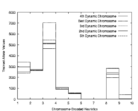
Figure 3: Top 5 dynamic chromosomes with allele values trained using dynamic fitness function.

A striking feature is the high variation of a single heuristic weight across different top chromosomes. The possible reasons for this observation include:

• strong correlation with a large variation in another optimal allele value,

• our training set is too small,

• a heuristic rule is used only rarely, and if it is applied, then it should dominate other rules, although by how much is not relevant.

Which of these explanations is appropriate would have to be studied for each of the alleles individually, but at least this diagram gives us some useful information as to which heuristic rules show high variation weights.

We also notice that some optimal heuristic weights have a large value while others have very small values (such as heuristic 6). This indicates that some heuristic rules appear to provide little additional information. Whether this is truly the case is an area for future study.

For each problem solved in the training set, GoTools returns the number of terminal leaves from that problem’s tree-search. How should these numbers be combined to calculate a fitness for all the problems in the training set? There are two ways in which we may construct a total fitness value:

1. all problems are given equal weight.

2. hard problems are favored over easy problems.

GoTools is already fast at solving easy problems, so it is natural to emphasize our optimization on the harder problems so we may solve them quicker in practice. Therefore, the performance of hard problems should have a greater influence on the fitness value. The measurements available, from which we must construct this fitness function, are the number of terminal leaves ($tl_{new}$) of the current chromosome, and the number of terminal leaves ($tl_{old}$) of a reference chromosome containing the pre-optimization heuristic weights. Several fitness functions were investigated, the four main ones are shown below:

• $$\mbox{fitness}=\sum_{\mbox{\scriptsize\ training problems}}\frac{(\mbox{tl}_{\mbox{\scriptsize\ old}})^{2}}{\mbox{tl}_{\mbox{\scriptsize\ new}}}$$ (1)

• $$\mbox{fitness}=\sum_{\mbox{\scriptsize\ training problems}}\frac{\mbox{tl}_{\mbox{\scriptsize\ old}}}{\mbox{\mbox{tl}}_{\mbox{\scriptsize\ new}}}$$ (2)

• $$\mbox{fitness}=\sum_{\mbox{\scriptsize\ training problems}}-\mbox{tl}_{\mbox{\scriptsize\ new}}$$ (3)

• $$\mbox{fitness}=\sum_{\mbox{\scriptsize\ training problems}}\frac{1}{\mbox{\mbox{tl}}_{\mbox{\scriptsize\ new}}}$$ (4)

After calculating the raw fitness values for each chromosome based on all problems in the training set, the fitness values of all chromosomes are shifted and linearly scaled to fit in the interval [0,1] so that the values are normalized for the GA’s selection function. With fitness functions (1), (2) and (3), the performance in solving harder problems has a higher impact in the fitness value. This behavior is desired as GoTools is already well optimized for small problems. Function (4) was included in our evaluation for reference purposes, as it does not favor hard problems. Comparisons between the four fitness functions showed that function (3) provides a good balance between larger and smaller problems. All results reported below were obtained using this fitness function. In principal, there is a danger of overemphasizing hard problems because their search tree is exponentially larger than the one of a simple problem. By counting the leaves of the search tree (i.e. measuring its surface) instead of counting all nodes (i.e. the volume of the search tree), we reduce this tendency of much larger values for slightly harder problems.

Finally, one must select the population size and number of children of each generation. Increasing the population size did not provide additional improvement as the heuristics are weakly linked and there are only ten dynamic heuristics to consider. Further, it was found that the best results were obtained with the number of children ideally matching the population size. Tests showed that population sizes and number of children on the order of 20 were most appropriate; since 24 nodes are available on our Beowulf cluster, we settled for 22 chromosomes forming the population size and number of children per generation (our parallel GA always requires an even number of children , plus the root node, thereby fully using our 24 node cluster). Our GA program is easily adjustable to support various population sizes, number of problems in the training set and the number of processors available to perform computations.

3 Results

Optimization of both the static heuristic weights and the dynamic heuristic weights provided improvements in search performance.

The static heuristic weights trained with the static fitness function did not provide any tangible improvement, and the results obtained indicate that a GA using this fitness function is only good at improving fitness weights, but not in solving other test sets of problems. However, static heuristic weights trained with the dynamic fitness function performed much better, giving an improvement of around 12% from the baseline (un-trained weights).

With a trained dynamic heuristic, an improvement of around 18% from the baseline (untrained weights) was achieved over many different types of problems. The optimized dynamic heuristic provides an 8% reduced terminal leaf count compared with that of the original heuristic weights. When combined with our trained static heuristic weights, the overall improvement is around 20%. These results are discussed in more detail in the following subsection.

The relatively moderate improvement achieved by optimizing heuristic weights is interpreted as follows. The strength of GoTools comes mainly from an early life and death detection, the use of a hash database to learn intermediate search results and other hard-wired learning mechanisms. The collection of heuristic rules is comparatively underdeveloped. Hence an improvement of weights can only have a limited value. The work to be done on improving the heuristic rules themselves will be much simplified with the genetic learning tools at hand which not only can fine-tune parameters but can also be used to judge the quality of the heuristic rules through a comparison of the achieved efficiency.

3.1 Static GA

Optimizing the static heuristics using only a static fitness function proved to be difficult, as the complexity of solving life & death problems is largely hidden from this function. Furthermore, as problem difficulty increases, the performance of the static heuristic deteriorates. The reason seems to be that difficult problems with many possible moves are not easily solved using simple heuristic rules and are therefore also not useful as training sets to learn the weights of simple heuristic rules. Therefore, to realize at least average results with the static heuristic, the training time becomes increasingly large as the population size must be increased accordingly. This indicates that the static heuristic function is not adequate to learn the solving of arbitrary test sets well.

Figure 4: Typical learning curve when training static weights with a static fitness function

Figure 4 shows a typical learning curve for the static heuristic function. The GA was run with a population size of 100 and a children size of 80, along with other parameters tuned as described in Section 2.5.1. Table 1 shows three runs using the static fitness function to optimize static weights with problems from the easy training set (lv3-6) tested on an easy test set (lv4-6) with three different training set sizes. The outcome that a training set size of 128 is slightly better than 200 is only a coincidence, but even if a training set size of 200 would have been slightly better, it would not have justified using a training set nearly twice as large. Based on this outcome, we used a training set size of 128 problems for the computation show in Figure 5.

In this Figure, the performance of three static heuristic sets, each trained with training sets of varying difficulty (lv3-6, lv3-10, lv3-14), is shown when tested with test sets of varying difficulty (lv4-6, lv4-10, lv4-14). The dominating feature of this diagram is the bad quality of weights trained with the difficult training set. Even if a larger GA population, more generations and a larger training set size might improve the performance, it is unlikely to reach the quality obtained with the dynamic fitness function.

Number of problems in training set:	64	128	200
Solution Leaves:	370,115	233,037	234,131

Table 1: Solution leaves of static weights trained with a static fitness function using the training set lv3-6 and the test set lv4-6 with varying training set sizes.

Figure 5: Solution leaves of static weights when trained with a static fitness function using a training set of 128 problems from lv3-6, lv3-10 and lv3-14 with varying test set (lv4-6, lv4-10, lv4-14) difficulty level.

As we suspected that the static fitness function was likely limiting the optimization of the static weights, the same static parameters were also optimized by completely solving the problems, that is, using the same fitness function as utilized in optimizing the dynamic parameters (see 2.5.2). We utilized a training set of 128 problems at various difficulty levels with a population size of 22 chromosomes and 22 children per generation. The GA was run for only 15 generations, and all other GA parameters remain the same as discussed earlier. This approach confirmed our suspicions, as shown in Figure 6.

Figure 6: Solution leaves of static weights when trained with a dynamic fitness function using a training set of 128 problems from lv3-6 and lv3-14 with varying test set (lv4-6, lv4-10, lv4-14) difficulty level.

The results shown in 6 indicate that, with a proper fitness function, the optimized static weights now perform clearly better. Furthermore, there is another useful trend evident in this diagram. We can see that the performance obtained when trained with easy problems (lv3-6) or hard problems (lv3-14) is very similar much in contrast to training with the static fitness function. Results obtained with a medium difficulty training set (lv3-10) also followed this trend, but are left out for graphical clarity. In fact, we can see that the heuristic weights trained with the easy problem set actually out-perform those trained with a hard problem set by a small margin.

Figure 7: Top 5 static chromosomes with allele values trained with dynamic fitness function.

Looking at the trained heuristic weights as shown in Figure 7, we can clearly see the difference to Figure 2 where the variance of allele values over the top five chromosomes is clearly higher. Although training with a dynamic fitness function which solves problems is much slower than using a static fitness function, this disadvantage is partially compensated by the fact that solving easy training sets, like lv3-6, is much faster than using a difficult training set. While not as fast as using a static fitness function, solving easy training set problems is still relatively quick on our Beowulf cluster, and much faster than training with a high difficulty training set as is required for the optimization of dynamic parameters, which is discussed below.

3.2 Dynamic GA

Obtaining a good dynamic heuristic can potentially bring a noticeable improvement to the already well-optimized GoTools tree-search. However, optimizing the dynamic heuristics involves solving the problem, which can quickly make such work very time consuming. A typical learning curve for the Dynamic GA is shown in Figure 8.

Figure 8: Typical learning curve when training dynamic weights with a dynamic fitness function.

We can see that for the training set used in Figure 8 that training with a dynamic fitness function is able to quickly converge. A training set of higher difficulty does tend to converge more slowly, but in general, 30 to 40 generations were sufficient. Figure 2 shows how the performance of the dynamic GA varies with training set size, as shown by the results obtained in training with 64, 128 and 200 problems taken from the full lv3-6 set.

Number of problems in training set:	64	128	200
Solution Leaves:	186,005	171,495	170,633

Table 2: Solution leaves vs. training set size when optimizing dynamic weights using the dynamic fitness function with lv3-6.

The table shows the solution leaves as reported when running a test set. There is a reasonable improvement of 8% achieved by increasing the size from 64 to 128 problems, while only a minor further improvement of 0.5% when increasing the size from 128 to 200 problems. When moving to more difficult problems, the improvement between a training set size of 128 and 200 problems does increase, however, overall a training set size of 128 problems is favorable in terms of results and the required computation time for training. Subsequently, we use a training set size of 128 problems for our main result, shown in Figure 9.

Figure 9: Solution leaves for zero dynamic parameters (baseline curve) and optimized dynamic parameters using lv3-6, lv3-10 and lv3-14 as test sets.

When optimizing static weights, it was advantageous to use easy problems for the dynamic fitness function. Conversely, here a high-difficulty training set is sufficient to perform well with an easy test set and necessary to perform well with a difficult test set. Therefore, we have trained with the lv3-14 training set with 128 problems, as shown in Figure 9. The baseline values are obtained by using un-trained dynamic parameters. The results shown indicate a 14%, 18% and 23% improvement in solution leaves at testing set difficulty levels of 6, 10 and 14 respectively. These results are consistent across many problem difficulty levels. The only requirement is to train with high difficulty training sets. Hence, the dynamic fitness function is preferred over the static fitness function as while training does take longer, it is only required once and can be well applied to a variety of problems with good results.

3.3 Profiling

Although the efficiency of the original heuristic weights were improved through the genetic learning of new weights, the improvement was not overwhelming. We now wish to analyze in greater detail the limiting behavior of our current heuristic rules. To this aim, we generated Figures 10 thru 14, which we refer to as profile plots.

Figure 10: Profile plot with baseline heuristic relative to original heuristic for easy, medium and hard difficulty level problems.

Figure 11: Profile plot with static heuristic (trained with static evaluation function) relative to original heuristic for easy, medium and hard difficulty level problems.

Figure 12: Profile plot with static heuristic (trained with dynamic evaluation function) relative to original heuristic for easy, medium and hard difficulty level problems.

Figure 13: Profile plot with dynamic heuristic relative to original heuristic for easy, medium and hard difficulty level problems.

Figure 14: Profile plot with best overall (combined) heuristic relative to original heuristic for easy, medium and hard difficulty level problems.

To create the profile plots shown in Figures 10 to 14, we ran five heuristics (our baseline, static weights optimized with the static evaluation function, static weights optimized with the dynamic evaluation function, dynamic weights and the new optimal (combined) heuristic) relative to GoTools’ existing (i.e. previously-optimal) heuristic on our library of $24,000$ problems. The x-axis measures the new leaf count compared with old leaf count = 100%. This means that problems measuring less than 100% improved (i.e. a reduction in leaf count), problems measuring greater than 100% became worse (i.e. an increase in leaf count) while problems close to 100% showed no performance change. The y-axis measures the number of problems counted at a given performance level, normalized to the range $[0,1]$. Our graphs are all plotted in the $x$-range $[0,300]$ once in the y-range $[0,1]$ and then again in the y-range $[0,0.1]$ only for better graphical clarity. Finally, we also selected our low, medium and high problem difficulty levels for the curves shown in each graph.

All of the profile plots shown indicate that very little change occurs for low difficulty problems. That is, there is no further optimization possible for solving low difficulty problems faster given the current heuristic rules implemented in GoTools. The single spike in the plots also indicates that the heuristic rules are adequate for these problems. As the difficulty level is increased, the behavior of these five heuristics changes noticeably. In Figure 10, we can see how much worse GoTools behaves without its heuristic rules as almost all of the profiled problems took longer to solve. By contrast, viewing Figure 11 confirms that using the static evaluation function to optimize the static weights resulted in an unstable profile with some problems being solved faster while most took longer to solve. Figure 12 shows improved results when the static heuristic was trained with the dynamic evaluation function. In this case, there is a higher concentration around the 100% mark which indicates this heuristic had a higher consistency across problems than the static heuristic trained with the static evaluation function. However, the results are still somewhat noisy, which is an indication of the limitation of the static heuristic rules.

The optimized dynamic heuristic shown in Figure 13 demonstrates the best behavior. There is some performance gained as the area below the curves is greater below the 100% level than the area above the 100% level. Furthermore, the results indicate a more consistent improvement across many problems when compared to the variable results seen with the static heuristics. The overall optimal heuristic shown in Figure 14 demonstrates a somewhat combined behavior which one may expect given that it is formed from the best dynamic and static heuristic weights learned. While it does have a lower consistency than the dynamic heuristics’ profile, the overall improvement still manages to give the best performance of all these evaluated heuristics.

Looking at the curves for higher difficulty problems the question arises why the optimized heuristics solve them so inconsistently. One reason is surely that solving life & death problems is intrinsically hard and there is no way to have simple heuristics which are good enough to solve hard problems without tree-search. On the other hand it must be said that the heuristic module of GoTools is one of the weak points of the program. The heuristic rules which currently are mainly based on superficial issues must be improved to show more understanding of what the situation is. Only then predictions for good moves will be valid for longer sequences of moves and therefore have value for more difficult problems.

To develop a better heuristic the profiling can be of good use. By setting all but one heuristic weight to zero and profiling the comparison with a run where all weights are zero allows one to filter out positions where a rule is counterproductive. By filtering out problems which are solved much slower when solved with one set of heuristic weights versus another set of weights, one obtains good examples where either individual rules or combinations of them become counterproductive.

A lesson learned so far is that dynamic rules are more generally applicable than static rules which seem to loose their predictive power for difficult problems, at least the rules implemented in GoTools currently.

4 Conclusion

The work described in this paper was meant to improve the current version of GoTools, as well as laying the groundwork for future development as the functionality of GoTools is widened to support the solving of open problems. The developed tools are:

• an MPI interface for Pascal (more specifically an MPICH implementation of it), run by us under FreePascal (http://www.freepascal.org) allowing the use of a Beowulf cluster for genetic learning or any other parallel computation (GoTools + infrastructure are written in Pascal.),

• a GA program that can use a static fitness function which computes heuristics, as well as dynamic fitness functions that solve problem training sets together with large sets of life & death problems of varying difficulty.

In terms of using these tools to improve the current version of GoTools, we worked on optimizing 2 sets of weights of heuristic rules.

Weights for static rules:

Because these rules take as input only the current board position we were able to use two different fitness functions. One fitness function, called static fitness, computes a heuristic ranking of all possible moves in a life & death problem and gives a bonus according to the place of the unique best move in this ranking. The other fitness function, called dynamic fitness, solves life & death problems and takes as fitness measure the negative of the number of terminal leaves of the search tree. Both fitness functions operate on a whole training set of problems for each single chromosome (i.e. set of heuristic weights). Our findings:

Using the static fitness function did not result in a good training of the static heuristic weights.

With the static fitness function, performance on the test set deteriorated as the problem difficulty was increased.

Using the dynamic fitness function, we found that training with an easy problem set was sufficient to obtain good performance on both easy and difficult test problems.

An improvement of 12% was realized when using the dynamic fitness function for our trained static heuristic weights as compared to zero weight values.

Weights for dynamic rules:

During the execution of GoTools different forms of learning take place. One is the filling of a hash data base with the status of intermediate positions, one is the rule that when backtracking then to try the other sides winning move first. These forms of learning are always performed. In addition there are other forms of learning (how often was a move a winning move in an intermediate position, negative bonus if a move is forbidden for the enemy,…). The value of these extra learning heuristics is not so clear cut and therefore heuristic weights are introduced for them. To optimize these weights the fitness function has to solve life & death problems. We found that

A high difficulty training set was sufficient to achieve good performance on easy test sets, and necessary to achieve good performance on difficult test sets.

An improvement of 18% was realized with our trained dynamic heuristic weights as compared to zero weight values, and an 8% improvement over the original dynamic parameter set was achieved with higher difficulty problems.

An overall improvement of 20% was realized when our trained static heuristic weights are combined with our trained dynamic heuristic weights.

5 Future Work

The emphasis of the computations done so far was to gather experience in using Genetic Algorithms to optimize heuristic weights in tsume go. One can push our results further by using more resources: larger population sizes, running the GA for more generations and using larger training sets. This will definitely be done once the heuristic module has been overhauled.

In our effort to genetically improve pruning parameters we still have to gather experience, especially in generating chromosomes evenly spread over a larger interval of speed-up levels. However, pruning parameters depend strongly on the quality of the static and dynamic heuristics and will become more important in the future when a new static heuristic module will be completed and be more effective for difficult open problems.

A more immediate task that emerged from our results is to critically analyze the different variance values of the optimized individual heuristic weights, and to check what can be learned about improving the heuristic rules themselves.

References

- [1] Koza, John R. (1992). Genetic Programming : On the Programming of Computers by Means of Natural Selection, MIT Press, Cambridge, Mass.
- [2] http://www-unix.mcs.anl.gov/mpi/mpich/
- [3] Pacheco, Peter S. (1998) A User’s Guide to MPI, Department of Mathematics, University of San Francisco.
- [4] http://www.beowulf.org/
- [5] Wolf, T. (2000). Forward pruning and other heuristic search techniques in tsume go, Information Sciences 122, no 1, 55–76.
- [6] Freund, John E. (2001). Mathematical Statistics, Fifth Edition, Prentice-Hall, Inc., New Jersey.