Searching for Plannable Domains can Speed up Reinforcement Learning

Abstract.

Reinforcement learning (RL) involves sequential decision making in uncertain environments. The aim of the decision-making agent is to maximize the benefit of acting in its environment over an extended period of time. Finding an optimal policy in RL may be very slow. To speed up learning, one often used solution is the integration of planning, for example, Sutton’s Dyna algorithm, or various other methods using macro-actions.

Here we suggest to separate plannable, i.e., close to deterministic parts of the world, and focus planning efforts in this domain. A novel reinforcement learning method called plannable RL (pRL) is proposed here. pRL builds a simple model, which is used to search for macro actions. The simplicity of the model makes planning computationally inexpensive. It is shown that pRL finds an optimal policy, and that plannable macro actions found by pRL are near-optimal. In turn, it is unnecessary to try large numbers of macro actions, which enables fast learning. The utility of pRL is demonstrated by computer simulations.

1. Introduction

1.1. Reinforcement Learning

Reinforcement learning involves sequential decision making in uncertain environments. The sequential aspect of the decision problem reflects the fact that the immediate cost or benefit of any state of the environment may play only a small part in determining the true value of any state. The aim of the decision-making agent is to develop a policy, which maximizes the benefit of acting in its environment over an extended period of time.

An often used and efficient framework, which describes stochastic, sequential decision problems, is the Markov decision process (MDP) (for a review, see [Puterman, 1994]). When a problem description satisfies the requirements of the MDP framework, well-known algorithms can be used to determine an optimal policy, such as various forms of the dynamic programming [Bellman, 1957, Bertsekas, 1987, Sutton, 1991], Q-learning [Watkins, 1989], or SARSA [Singh and Sutton, 1996] methods.

These algorithms proceed by maintaining a value function, updating it according to the experiences and propagating the values of states. Under appropriate conditions, RL algorithms are shown to develop an optimal policy [Bertsekas, 1987, Singh et al., 2000]. However, the basic forms of these algorithms propagate the values step-by-step, therefore convergence may be very slow. Various methods have been developed to overcome this difficulty, such as prioritized sweeping [Moore and Atkeson, 1993], eligibility traces [Sutton, 1988, Singh and Sutton, 1996] and also planning methods to be described below.

1.2. Planning

Besides RL, another successful and well-studied approach to solving decision problems is planning. As a central problem of classical AI research, effective algorithms have been developed to solve planning problems. However, classical decision-theoretic methods usually assume that the world is deterministic. This is an appropriate approximation in some cases, but not always. There may be certain parts of the world, that are highly stochastic, making classical planning unreliable, or even useless. It is a plausible idea to integrate planning and reinforcement learning to gain more general and robust methods.

Sutton and colleagues as well as others [Sutton, 1991, Sutton, 1990, Peng and Williams, 1993, Forbes and Andre, 2000] have integrated planning and learning in the Dyna architecture: Planning is treated as being virtually identical to reinforcement learning. Learning updates the appropriate value function estimates according to experience as it actually occurs, whereas planning updates the same value function estimates for simulated transitions chosen from the world model.

Other researchers [Sacerdoti, 1977, Korf, 1985] used planning to develop macro actions (i.e., fixed sequences of actions) that could speed-up value propagation and learning. A macro action could be a complete sub-policy (such as ‘go to the door’, ‘search a wall’, etc.) [Hauskrecht et al., 1998, Precup et al., 1998, McGovern and Sutton, 1998]. The main difficulty with macro actions is how to construct them: they must be either handcrafted (see, e.g., [Kaelbling, 1993, Kalmár et al., 1998]) or one must try to generate them automatically (see, e.g., [Dietterich, 2000]). In this latter case a great number of useless macros might be generated, which might even deteriorate learning [McGovern and Sutton, 1998, Kalmár and Szepesvári, 1999].

1.3. Thesis of the Paper

We propose a method called plannable RL (pRL), that has similarities with both planning methods mentioned: we make focused value updates based on hypothetical experiences gained from a model. This is similar to the Dyna architecture. On the other hand, we maintain two separate (but interacting) value functions, one for learning and one for planning. We use a simple model to evaluate the value function for planning: values are updated when transitions are considered plannable (i.e., when those are close to deterministic). This planning-value function is then used to compute macro actions. We show that these macro actions are near-optimal. This means that we do not need to generate large numbers of (possibly bad) macro actions, and fast learning is still possible.

1.4. Structure of the Paper

First, the basis of RL methods are reviewed (Section 2. The pRL algorithm is described and a pseudo-code of the algorithm is provided in Section 3. The near optimality of the algorithm is proven in Section 4. Computational demonstration are provided in the next section, i.e., in Section 5. The paper is finished by a discussion (Section 6).

2. Preliminaries

2.1. Reinforcement Learning (RL) and the MDP framework

Let us recall the definition of a Markov decision process (MDP) [Puterman, 1994]. A (finite) MDP is defined by the tuple $\langle X,A,R,P\rangle$, where $X$ and $A$ denotes the finite set of states and actions, respectively. $P:X\times A\times X\rightarrow[0,1]$ is called the transition function; $P(x,a,y)$ gives the probability of arriving at state $y$ after executing action $a$ in state $x$. Finally, $R:X\times A\rightarrow\mathbb{R}$ is the reward function, $R(x,a)$ gives the immediate reward for choosing action $a$ in state $x$.

At each sequence of discrete time steps, $t=0,1,\ldots$, the problem-solving agent observes its world to be in state $s_{t}\in S$ and executes an action $a_{t}\in A$. After this action, the agent receives reward $r_{t+1}\in\mathbb{R}$ from the world and observes the next state, $s_{t+1}$ according to the functions $R$ and $P$.

The agent’s objective is to choose each action $a_{t}$ so as to maximize the expected discounted return, $\mathcal{R}_{t}$, i.e., $E\left(\mathcal{R}_{t}=r_{t+1}+\gamma r_{t+2}+\gamma^{2}r_{t+3}+\ldots\right)$, where $0\leq\gamma<1$ is the discount factor and $E(.)$ denotes the expected value of the argument.

A Markovian policy $\pi$ is a $S\times A\to[0,1]$ mapping, where $\pi(x,a)$ is the probability that in state $x$ the agent selects action $a$. The value of a state $x$ under policy $\pi$ is the expected value of the total discounted reward of starting from $x$ and then following policy $\pi$. Formally, $V^{\pi}(x)=E_{P,\pi}(\sum_{t=0}^{\infty}\gamma^{t}r_{t}|s_{0}=x)$ (i.e., the expected value depends on the transition probabilities and the policy applied). These values satisfy the recursive equations

$$V^{\pi}(x)=\sum_{a\in A}\pi(x,a)\left(R(x,a)+\gamma\sum_{y\in S}P(x,a,y)V^{\pi}(y)\right)\text{ for all }x.$$

A policy $\pi^{*}$ is optimal, if for all policies $\pi$, $V^{\pi^{*}}(x)\geq V^{\pi}(x)$ for all $x\in S$ (it is easy to show that such a policy exists). The corresponding value function satisfies

(2.1) $$V^{*}(x)=\max_{a\in A}\left(R(x,a)+\gamma\sum_{y\in S}P(x,a,y)V^{*}(y)\right).$$

A standard way to find an optimal policy is to compute the optimal value function $V^{*}:X\rightarrow\mathbb{R}$, which gives the value (i.e., the expected accumulated discounted reward) for each starting state. From $V^{*}$, the optimal policy can be derived: the ‘greedy’ policy with respect to the optimal value function is an optimal policy (see, e.g., [Sutton and Barto, 1998] and references therein). This is the well-known value iteration approach [Bellman, 1957]. Functions $V^{\pi}$, $V^{*}$ are called value functions, which are associated with a fixed policy $\pi$ and with the optimal policy, respectively.

We can also define the action value function $Q^{\pi}(x,a)$ as the expected value of the total discounted reward of starting from state $x$, choosing action $a$ and then following policy $\pi$. This value function is often more useful, because it provides the values of individual actions. It is easy to see that

$$Q^{\pi}(x,a)=R(x,a)+\gamma\sum_{y\in S}P(x,a,y)V^{\pi}(y),$$

$$V^{\pi}(x)=\sum_{a\in A}\pi(x,a)Q^{\pi}(x,a)$$

and thus

$$Q^{\pi}(x,a)=R(x,a)+\gamma\sum_{y\in S}P(x,a,y)\sum_{a^{\prime}\in A}\pi(y,a^{\prime})Q^{\pi}(y,a^{\prime}).$$

The optimal action-value function $Q^{*}$ satisfies an equation analogous to $V^{*}$:

$$Q^{*}(x,a)=R(x,a)+\gamma\sum_{y\in S}P(x,a,y)\max_{a^{\prime}\in A}Q^{*}(y,a^{\prime}).$$

2.2. Dynamic Programming and Two Basic RL Algorithms

Equation 2.1 can be used as an iteration:

(2.2) $$V_{t+1}(x)=\max_{a\in A}\left(R(x,a)+\gamma\sum_{y\in S}P(x,a,y)V_{t}(y)\right)$$

for every state $x$, and for an arbitrary $V_{0}$. The iteration is known to converge to $V^{*}$. The method is called value iteration.

If the model of the environment (i.e. $R$ and $P$) is not known, or the state space is too large for solving Eq. (2.2), then sampling methods can be used. One such algorithm is called Q-learning [Watkins, 1989]. Q-learning uses the following iteration:

(2.3) $$Q_{t+1}(s_{t},a_{t})=(1-\alpha_{t})Q_{t}(s_{t},a_{t})+\alpha_{t}\left(r_{t}+\gamma\max_{a\in A}Q_{t}(s_{t+1},a)\right),$$

where $s_{t}$, $a_{t}$ and $r_{t}$ are the state of the system, the selected action, and the immediate reward at time step $t$, respectively, $Q_{0}$ is arbitrary, and $0\leq\alpha_{t}\leq 1$ is the learning rate.

It has been shown that if $\alpha_{t}$ converges to 0 properly ($\sum_{t}\alpha_{t}$ is divergent, but $\sum_{t}\alpha_{t}^{2}$ is convergent), and if every $(x,a)$ pair is updated infinitely often, then $Q_{t}$ converges to $Q^{*}$ with probability 1. The proof can be found, e.g., in [Singh et al., 2000].

Another RL method is SARSA, which takes sampling to the extreme. It has an update rule similar to (2.3):

(2.4) $$Q_{t+1}(s_{t},a_{t})=(1-\alpha_{t})Q_{t}(s_{t},a_{t})+\alpha_{t}\left(r_{t}+\gamma Q_{t}(s_{t+1},a_{t+1})\right),$$

where $Q$-values of the iteration are action value estimates of two state-action pairs, the one which just occurred and its predecessor. SARSA is convergent under the same assumptions as Q-learning [Singh et al., 2000]. A comprehensive overview of various reinforcement learning methods can be found in [Sutton and Barto, 1998] and in the references therein.

2.3. Planning with Dyna

Reinforcement learning often requires a large number of experiences (i.e. $(s_{t},a_{t},r_{t},s_{t+1})$ tuples) to develop an appropriate policy. This is efficient when experience can be collected quickly, provided that one can afford the cost of explorations. Dyna offers a solution to improve the exploitation of previous experiences by integrating planning into the learning process.

Informally, planning is a process of computing a (near-)optimal policy for the existing (possibly inaccurate) model of the environment. Planning is an off-line method, it improves the policy without invoking additional interactions with the environment. DP, for example, executed on the available model, is a planning algorithm. Limitation arises if the model is not given: experience is needed to build a model. Another problem appears when DP is computationally intensive: performing a single and complete DP iteration requires $O(|S|^{2})$ computation steps. Efforts have been made to overcome this drawback, yielding solutions like prioritized sweeping [Moore and Atkeson, 1993], or real-time dynamic programming [Barto et al., 1995].

Another successful approach is to combine reinforcement learning and dynamic programming in a single algorithm. This approach was first suggested by Sutton, who called the algorithm Dyna. The basic idea is that one DP update on one single state can be interpreted as a reinforcement learning step. In the Dyna architecture the agent repeats the following steps: (1) obtain experience from the environment, (2) use this to update the value function, (3) use the experience to improve the model of the environment (e.g. to approximate the transition probabilities), (4) obtain hypothetical experience from the updated model, and (5) use the hypothetical experience to update the value function. Note that Dyna focuses DP iterations on previously visited (and thus presumably important) regions of the state space, and therefore it might reduce the computational demand of DP significantly.

Dyna allows the adjustment of planning relative to collecting experiences: if there is no time for planning, steps (4) and (5) can be omitted. Conversely, if real experience is slow or costly, then multiple planning steps may be accomplished.

2.4. Planning with Macro Actions

Another possibility for utilizing additional computational capacity is to compile compound actions (macro actions) from basic ones. In its simplest form, macros are fixed sequences of actions (e.g. ‘go forward, turn right, go forward’). Many works have dealt with different versions of the macro concept. In particular, one might consider policies of sub-problems (e.g., policy for ‘finding a wall’ or policy for ‘going to the door’) as macros. In this case separate value functions on separate parts of the state-space will arise.

In order to integrate macros into reinforcement learning, two additional steps must be implemented: (6) the generation of macro actions and (7) the evaluation of macro actions. The latter one can be accomplished, e.g., by computing $Q(x,a_{\textrm{macro}})$ in all necessary states. Generating appropriate macro actions is a more difficult problem. One commonly used approach is to pre-wire them by hand [Kaelbling, 1993]. This is a straightforward way to encode prior knowledge into the learning problem if such prior knowledge is available and if the environment is steady. Efforts have been made also to generate macro actions in an automated fashion. The general approach is to use some heuristics to compile a number of macros from basic actions, evaluate the macros, and then keep the ones which are the most useful.

A useful set of macro actions can substantially speed up learning, because the agent can make larger steps toward its goal. On the other hand, evaluating bad macros can deteriorate performance (because trying a bad macro takes a large step in a wrong direction).

3. The pRL algorithm

In this section a novel algorithm is proposed, which combines DP and macros. First, a model is built for model-based value-function updates, just like in Dyna. These updates are used directly to find useful macro actions and to calculate their utility. A parallel approximate value function is maintained, which encodes the macros and their values according to the model. Greedy policy with respect to this approximate value function is applied. The resulting policy is then used to choose a macro action.

An important question is the choice of the model. One might attempt to learn an approximation of the $P(x,a,y)$ transition probabilities and the corresponding rewards. However, estimating and maintaining a table of size $|S|^{2}\cdot|A|$ may not be feasible. Finally, we think that planning is more effective in near-deterministic domains of the state space, and is less advantageous when little is known about the outcome of an action. Such problems frequently arise in real life. For example,

• when one has to pass a city, one might choose going through the city directly or taking the ring around the city. The first option could be less expensive in many cases, but large durations on travel time may arise if a traffic jam occurs in the inner areas. The second option may allow for more accurate planning and may have a competitive cost on the average.

• Requests can be distributed for mobile agents in many different ways. Planning becomes crucial when part of the system may be(come) unreliable.

Our planning algorithm (the planner) stores only those transitions that are almost deterministic, which we shall call plannable transitions. The algorithm will be called plannable-RL, or pRL, for short.

3.1. Basic Definitions, the Value Functions and their Update Rules

In the following we specify the pRL algorithm. First of all, we define plannable transitions formally:

Definition 3.1.

A transition $(x,y)$ is called plannable with accuracy $\kappa$, if it can be realized with probability $\kappa$, i.e. there exists an action $a(x,y)$ such that $P(x,a(x,y),y)\geq\kappa$.

Let us denote the set of states that are plannable from state $x$ by $T(x)$, i.e.

$$T(x):=\{y:(x,y)\ \textrm{is $\kappa$-plannable}\}=\{y\mid\exists a(x,y):P(x,a(x,y),y)\geq\kappa\}$$

We assume that we are given an inverse dynamics $\phi:X\times X\to A$ such that $\phi(x,y)=a(x,y)$, if $(x,y)$ is plannable, and it is arbitrary otherwise. This is a reasonable assumption; either the inverse dynamics is known in advance, or, the ‘learning by doing’ method can be sufficient to approximate the inverse dynamics for the plannable domains.

To compute $T(.)$, we approximate $P(x,\phi(x,y),y)$ with $\hat{P}_{t}(x,y)$ using the following approximation scheme:

(3.1) $$\hat{P}_{t+1}(x,y)=\begin{cases}(1-\alpha_{t})\hat{P}_{t}(x,y)+\alpha_{t}\cdot 1&\text{if $s_{t}=x$, $a_{t}=\phi(x,y)$ and $s_{t+1}=y$},\\ (1-\alpha_{t})\hat{P}_{t}(x,y)+\alpha_{t}\cdot 0&\text{if $s_{t}=x$, $a_{t}=\phi(x,y)$ and $s_{t+1}\neq y$},\\ \hat{P}_{t}(x,y)&\text{otherwise},\end{cases}$$

$$\hat{P}_{0}\equiv 1.$$

Note that this iteration approximates the exact transition probabilities. A transition $(x,y)$ is considered plannable, iff $\hat{P}_{t}(x,y)\geq\kappa$. These almost-sure transitions will be considered as sure by our planning algorithm. The approximation simplifies the required computations, and – as we shall show later – provides near-optimal solutions.

Definition 3.2.

Connected components of plannable transitions are called plannable domains.

Note that plannable domains are disjoint. In turn, the number of plannable domains is smaller than the number of states.

The immediate rewards of plannable transitions are similarly approximated by $\hat{R}(x,y)$.

In our algorithm, two value functions are maintained: a standard (basic) action-value function $Q(x,a)$, $a\in A$, which is updated by real experiences, and another value function called the planning value function. The planning value function will make use of a Dyna-like algorithm above the simplified model described in Eq. (3.1). Both functions suggest – possibly different – policies. In every time step, pRL can switch between these policies by examining which one seems better.

3.2. Updating the basic value function

For updating the basic value function, any traditional RL update rule can be applied. For example, one may use DP, Q-learning, SARSA, etc. We use SARSA because of its simplicity:

$$Q_{t+1}(s_{t},a_{t})=(1-\alpha_{t})Q_{t}(s_{t},a_{t})+\alpha_{t}\left(r_{t}+\gamma Q_{t}(s_{t+1},a_{t+1})\right),$$

where $s_{t}$, $a_{t}$ and $r_{t}$ are the state of the system, the selected action and the reward at time step $t$, respectively. $Q_{0}$ is arbitrary, and $0\leq\alpha_{t}\leq 1$ denotes the learning rate. Note that the basic value of state $x$ at time $t$ is given by $V_{t}(x)=\max_{a}Q_{t}(x,a)$.

3.3. Updating the planning value function

Several update rules could be used for the planning value function. However, there is an important difference: an (approximate) model and an inverse dynamics is known for this case. Therefore We do not need to maintain an action-value table, instead a simple state value function can be used. This function will be denoted by $\hat{V}(x)$. The corresponding policy can be determined, e.g., by the inverse dynamics. Note that this policy may differ from the policy suggested by the basic value function.

We chose the value iteration update rule in the following form:

$$\hat{V}_{t+1}(x)=\max_{a}\sum_{y}(P(x,a,y)(R(x,a,y)+\gamma^{\prime}\hat{V}_{t}(y))).$$

The number of non-vanishing terms of this update may be considerably smaller than the number of all possible terms, because in our approximate model all transition probabilities are either 0 or 1. Transitions with low probability are omitted, whereas transitions with high probability (determined by $\kappa$) are considered as sure transitions. Note that this simplification could mislead action selection. The error depends on the degree of the simplification, which is determined by $\kappa$: lower $\kappa$ results in a coarser model. Assuming that immediate reward $R$ is approximated by $\hat{R}_{t}$, the update rule can be rewritten as

(3.2) $$\hat{V}_{t+1}(x)=\max\left\{\max_{y\in T(x)}(\hat{R}_{t}(x,y)+\gamma^{\prime}\hat{V}_{t}(y)),V_{t}(x)\right\}.$$

Here we took into consideration that sometimes it is better to select actions according to the basic value function $V_{t}(x)$ (i.e. continue sampling or quit planning and start sampling) than to select action according to the planning value function $\hat{V}_{t}(x)$) (i.e., continue planning, or quit sampling and start planning). Note that when no plannable states are available, one has to return to the basic value function. One may think of this technique that the space of plannable actions is extended by a new pseudo-action, which could be called ‘stop planning’: The choice of this action retreats to sampling and to action selection by means of the basic value function.

The update rule is applied for the planning value action in the plannable area around the current state $x$ in every time step. This area can be determined by a limited breadth-first search on the graph of plannable transitions, starting from state $x$. The search phase and the update phase require no interactions with the real system, these are ‘off-line’ evaluations. Due the to limited search and the limited number of DP updates, they take only $\mathcal{O}(C)$ steps.

3.4. Action selection

In classical RL methods (Q-learning, SARSA, etc.), $\varepsilon$-soft or $\varepsilon$-greedy policies with respect to the actual value function can serve to support exploration and exploitation (see, e.g., [Sutton and Barto, 1998]). Now we have two different value functions which may suggest different policies. We shall make use of the $\varepsilon$-greedy policy when $Q_{t}$ is used, but if the value of planning from the actual state is higher, i.e. $\hat{V}_{t}(x)>V_{t}(x)$, then action will be generated by means of the planning value function $\hat{V}_{t}$. This decision is made by pRL in every state.

3.5. Plannable transitions as macros

Macros are not represented explicitly in pRL, only through the planning value function. This is advantageous because we do not need much space to store the macros - and we can still store the most useful macro with its value for each state.

The macro encoded by $\hat{V}$ is ”choose the greedy action according to $\hat{V}_{t}$, while $\hat{V}_{t}>V_{t}$. Stop macro, if an action leads to a state other than the planned one.”

More formally, let

$$S(x):=\arg\max_{y}(\hat{R}_{t}(x,y)+\gamma^{\prime}\hat{V}_{t}(y))$$

be the greedy selection according to $\hat{V}$, and let

$$a(x):=\phi(x,S(x)).$$

Then the macro of state $x$ is the action sequence $a(x),a(S(x)),a(S(S(x))),\ldots,a(S^{n}(x)),\ldots$, with the stopping condition ”stop at the $n$th step, if either $\hat{V}_{t}(S^{n+1}(x))<{V}_{t}(S^{n+1}(x))$, or taking action $a(S^{n}(x))$ in state $S^{n}(x)$ leads to a state other than $S^{n+1}(x)$.

Naturally, such listing of the macros can be included into the pRL algorithm, but is not necessary.

The pseudo-code of the algorithm is summarized in Fig. 1.

Figure 1. Pseudocode of the pRL algorithm. In this form, the algorithm takes at most $\mathcal{O}(N+M)$ steps for every action selection.

4. Near-optimality of pRL Macros

It is easy to see that the basic value function of pRL converges to the optimal value function. This follows from the fact that the convergence theorem for SARSA and Q-learning [Singh et al., 2000] requires (i) sufficient exploration (every $(x,a)$ pair should be visited infinitely often) and (ii) setting the learning rate properly ($\sum_{t}\alpha_{t}=\infty$, but $\sum_{t}\alpha^{2}_{t}<\infty$). Clearly, if these criteria are satisfied with standard RL algorithms, then they are also satisfied in pRL. However, convergence to the optimal policy is guaranteed only if macros are valued correctly, i.e., if $\kappa=1$. The rate of convergence can also be seriously affected by $\kappa$: $\kappa<1$ allows for a larger set of macros and may converge much faster to (possibly suboptimal) solutions. Therefore, it is an important issue how the learning and the utilization of macros will influence performance. For the analysis of this problem, an extension of the classical MDP model is necessary. For this reason, we briefly introduce $\varepsilon$-MDPs [Szita et al., 2002b], and review related theorems. The $\varepsilon$-MDP-theory will be applied to pRL to show that macros are near-optimal.

4.1. $\varepsilon$-MDPs

The RL problem can be extended so that the environment is no longer required to be an MDP, it is only required to remain ‘near’ to an MDP, i.e. the environment is allowed to change over time, even in a non-Markovian manner.

The closeness of two environments (which have the same state- and action-sets) is measured by the distance of their transition functions. We say that the distance of two transition functions $P$ and $P^{\prime}$ is $\varepsilon$-small ($\varepsilon>0$), if $\|P(x,a,.)-P^{\prime}(x,a,.)\|_{L_{1}}\leq\varepsilon$ for all $(x,a)$, i.e. $\sum_{y}|P(x,a,y)-P^{\prime}(x,a,y)|\leq\varepsilon$ for all $(x,a)$. (Note that for a given state $x$ and action $a$, $P(x,a,y)$ is a probability distribution over $y\in X$.)

A tuple $\langle X,A,\{P_{t}\},R\rangle$ is an $\varepsilon$-MDP with $\varepsilon>0$, if there exists an MDP $\langle X,A,P,R\rangle$ (called the base MDP) such that the difference of the transition functions $P$ and $P_{t}$ is $\varepsilon$-small for all $t=1,2,3,\ldots$.

As a simple example for an $\varepsilon$-MDP, consider an ordinary MDP perturbed by a small noise in each time step.

4.2. Convergence of Learning Algorithms in $\varepsilon$-MDPs

One expects that such small perturbations in the environment may not disturb the performance of the learning algorithms very much. Nevertheless, one cannot expect that any algorithm finds an optimal value function in an $\varepsilon$-MDP. (Such a solution may not even exist because of the perturbations of the environment). However, we shall guarantee that these algorithms find near-optimal value functions. Formally, the task is to show that $\lim\sup_{t\to\infty}\|V_{t}-V^{*}\|\leq\textit{const}\cdot\varepsilon$ (or $\lim\sup_{t\to\infty}\|Q_{t}-Q^{*}\|\leq\textit{const}\cdot\varepsilon$), where $V^{*}$ and $Q^{*}$ are the optimal value functions of the base MDP.

First, consider Q-learning. Recall the update:

(4.1) $$Q_{t+1}(x_{t},a_{t})=(1-\alpha_{t}(x_{t},a_{t}))Q_{t}(x_{t},a_{t})+\alpha_{t}(x_{t},a_{t})(r_{t}+\gamma\max_{a}Q_{t}(\tilde{y}_{t},a)),$$

where $\tilde{y}_{t}$ is selected by sampling, i.e., according to the probability distribution $P_{t}(x_{t},a_{t},.)$.

Theorem 4.1.

Let $Q^{*}$ be the optimal value function of the base MDP of the $\varepsilon$-MDP, and let $M=\max_{x,a}Q^{*}(x,a)-\min_{x,a}Q^{*}(x,a)$. If

1. every state-action pair $(x,a)$ is updated infinitely often,

2. the learning rates satisfy $\sum_{t=0}^{\infty}\chi(x_{t}\!=\!x,a_{t}\!=\!a)\alpha_{t}(x,a)=\infty$ and $\sum_{t=0}^{\infty}\chi(x_{t}\!=\!x,a_{t}\!=\!a)\alpha_{t}(x,a)^{2}<\infty$ uniformly w.p.1,

then $\limsup_{t\to\infty}\|Q_{t}-Q^{*}\|\leq\frac{2}{1-\gamma}\gamma M\varepsilon$ w.p.1.

The proof can be found in [Szita et al., 2002a].

The case of SARSA. The proof of the near-optimality of the SARSA update is similar to the proof of Q-learning. Here it suffices to refer to [Singh et al., 2000]: It has been proven for MDPs in [Singh et al., 2000] that if Q-learning converges to the optimal value function, then – under the same conditions – SARSA converges, too. The proof in [Singh et al., 2000] carries over directly to $\varepsilon$-MDPs [Szita et al., 2002a].

4.3. pRL in the $\varepsilon$-MDP Framework

Recall that for finding macro actions, we have applied learning methods that find optimal policies and value functions in the modified environment, where almost sure transitions (with probabilities greater than $\kappa$) are treated as sure (probability 1). It may be worth noting that according to Eq. 3.2 the value function of the model (i.e., $\hat{V}$) is inherited from the original value function. $\hat{V}(x)$ can be different from $V(x)$ iff $P(x,y)$ is modified by the model. Note that modification of $P(x,y)$ is at most $\varepsilon$. Therefore the modified environment is an $\varepsilon$-MDP of the original one, with $\varepsilon=1-\kappa$, so one can apply the $\varepsilon$-MDP-theory to prove the following:

Corollary 4.2.

The pRL algorithm that uses either DP, Q-learning or SARSA for the learning of the macro-value function, produces approximations $\hat{V}_{t}$ such that $\lim\sup_{t\to\infty}\|\hat{V}_{t}-V^{*}\|\leq\textit{const}\cdot(1-\kappa)$.

Consequently, the macro actions found by pRL are asymptotically near-optimal.

5. Experiments

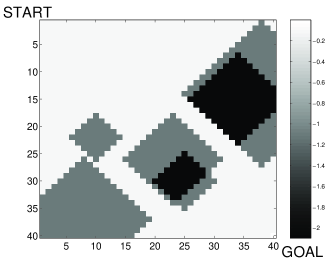
(a) Immediate rewards of the example labyrinth. The colors mark the gained immediate reward when the agent arrives in a the plotted states. Reaching the goal state means an immediate +200 reward (this one is not depicted on this picture).

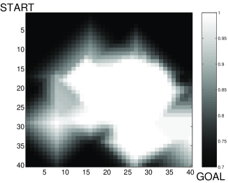
(b) Probabilities in the example labyrinth. The colors mark the probability by which an action leads to the ’good’ state from the plotted states, e.g. if selecting the action ’NORTH’ the agent in a given state, the agent really arrives in the state lying northward. If the transition is not successful in this sense, the agent arrives in a ’bad’ state chosen with equal probability from the other possible next states.

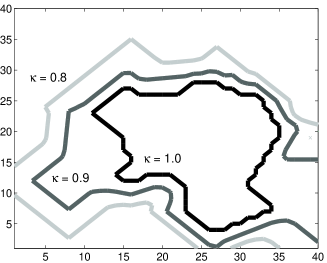
(c) Plannable areas at different $\kappa$

Figure 2.

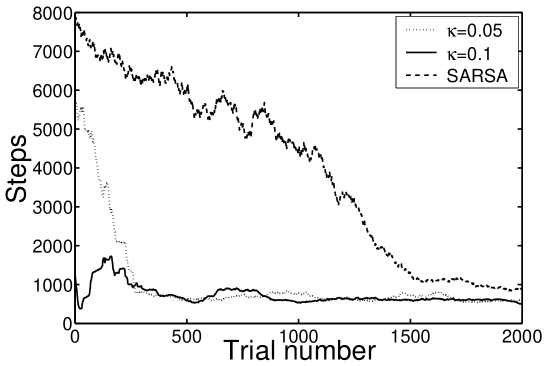
Figure 3. Convergence Speed of pRL
Learning curves for three different kappa values. Dotted line: $\kappa=0.05$, solid bold line: $\kappa=0.15$, dashed bold line (SARSA): $\kappa=1.0$. The curves represent averaged step numbers using averaging over 500 steps. Planning converges much faster then the original SARSA in the early phase. Convergence, however, continues beyond 2000 trials.

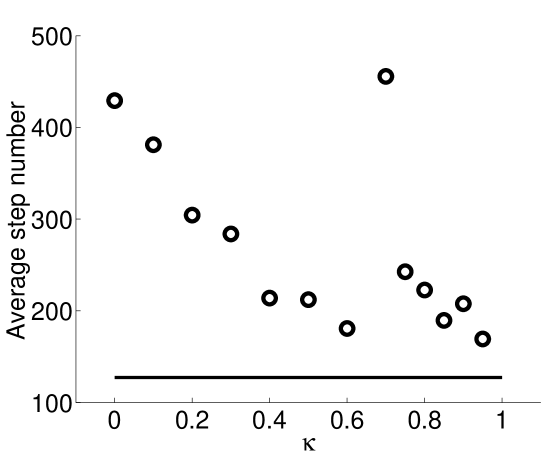
Figure 4. Optimality of pRL
Final performance of the resulting policy as a function of $\kappa$ values. Upon training has converged, the performance of the algorithm was measured by averaging the number of steps (in 10000 trials) required to finish one trial. The horizontal line depicts the optimal solution found by SARSA ($\kappa=1$).

To test pRL, a $40\times 40$ maze was generated. The agent starts in the upper left corner and its goal is in the lower right corner. In every state, the agent observes its position and can take four different actions (N(=north),S(=south),E(=east), and W(=west)). In every state $s$, an action is successful with probability $P^{succ}(s)$ if the attempted direction is successfully executed, and it fails with probability $1-P^{succ}(s)$ when the agent steps to a random, wrong direction. A lower bound for $P^{succ}(s)$ was set to 0.7. Regions with higher $P^{succ}(s)$ were generated. The probability of $P^{succ}(s)$ was gradually increased to 1 within these regions. The agent received a small $(-0.1)$ negative reward in each state, except for the goal state, where it received the reward of $+200$. In addition, some pitfall domains were generated randomly. Every domain contributed to the local reward by $-1$. In case of overlaps amongst the domains rewards were cumulated. After reaching the goal, a new episode was started. An example problem is shown in Fig. 2.

In the experiments, SARSA was utilized with $\varepsilon$-greedy action selection, with eligibility traces ([Sutton, 1988, Singh and Sutton, 1996]). The following parameters were used: learning rate was held constant at $\alpha=0.001$. The eligibility decay $\lambda$ was set to $0.95$, discount factor $\gamma$ was equal to $0.98$, the probability of random action selection was $0.1$. For pRL, the same setting was used and several $\kappa$ values were tried. The number of updates was set to 10.

5.1. Convergence speed

In theory, by setting $\kappa=1$, pRL becomes identical to SARSA, and by setting $\kappa=0$, pRL becomes equivalent to the simplest Dyna algorithm (see 3.1). By choosing an appropriate $\kappa$, pRL learns at least as quickly as the better candidate, thus it approximates the convergence rate of Dyna – which usually converges in a few trials in this case – even at low $\kappa$ values (Fig. 3). Problems may arise if it is not known whether the best solution corresponds to total planning (Dyna) or if no planning is possible at all (SARSA). By choosing an appropriate $\kappa$, (or a set of $\kappa$’s) the convergence rate of pRL can always achieve these boundaries. The method is most useful if computations for different $\kappa$’s can be afforded.

5.2. Optimality

The second experiment demonstrates the near-optimality of pRL. The performance of the resulting policy for different $\kappa$ values were computed (Fig. 4). The question is the value of the constant multiplier of Corollary 4.2; whether it is too high or not. Here, the assumption about deterministic transitions does not significantly influence the performance for high $\kappa$ values, as expected. It was also found that the resulting policies perform quite well for some fairly low $\kappa$ values; for example, $\kappa\approx 0.5$ performed still reasonably well. This suggests that better (stronger) estimations might exist for this problem. However, there is a $\kappa$ region, which exhibits poor performance. This region is around $\kappa=0.7$. The poor performance is the consequence of the special properties of our toy problem. In this $\kappa$ region, learning is compromised by the fact that most transition probabilities had a value of 0.7 (except in the plannable domains), and thus the algorithm had large uncertainties whether a particular transition is plannable or not.

6. Discussion

In this work, we introduced a new algorithm called pRL, which integrates planning into reinforcement learning in a novel way. An attractive property of our algorithm is that it can find near-optimal value function and near-optimal policy under certain conditions. Furthermore, the macros created by pRL are near-optimal. Near-optimality is controlled by the certainty of planning: our algorithm deals with $kappa$-plannable transitions, which have transition probabilities $0<\kappa\leq 1$.

Our algorithm was illustrated by computer simulations on a toy problem. It was found that SARSA is slow, but it leads to optimal solutions. On the other hand, Dyna may be fast but the resulting policies could be poor. Our algorithm incorporates both SARSA and Dyna. These are the extremes, SARSA corresponds to $\kappa=1$, whereas the original form of Dyna [Sutton, 1991] is recovered when $\kappa=0$. By tuning $\kappa$ in pRL and by using the arising computationally inexpensive model of pRL, one can quickly find almost optimal solutions. This feature is most advantageous when off-line computations are inexpensive. Comparisons amongst the different methods are provided in Table 1.

	DP is unexpensive	DP is expensive	DP is expensive
	new data is expensive	new data is unexpensive	new data is expensive
SARSA	slow, optimal	fast, optimal	slow, optimal
Dyna	fast, optimal	slow, optimal	slow, optimal
simple Dyna	fast, not optimal	slow, not optimal	slow, not optimal
pRL	fast, near-optimal	fast, near-optimal	fast, near-optimal
	(low $\kappa$)	(high $\kappa$)

Table 1. Comparison of RL methods for various problem types. ‘Cheap DP’ means that DP iterations have low computational cost, e.g., because the state space is relatively small. ‘New data is cheap’ means that the agent can easily obtain new experience by interacting with the environment. ‘Optimal’ means that the method eventually converges to an optimal policy.

pRL fits well into existing planning paradigms: it can be seen as a prioritized sweeping method where only the plannable states (i.e. states which can be reached almost deterministically from the current state) are updated. In turn, our method is a particular (extended) form of prioritized sweeping (see, e.g. [Moore and Atkeson, 1993]). One can decide to select updates according to state values [Moore and Atkeson, 1993], to select updates ordered by increasing distance from the current state or by prediction difference [Peng and Williams, 1993]. Prioritized sweeping can dramatically improve the performance of planning. Using our method, one cane also have performance bounds.

pRL can support approaches aiming to solve partially observable Markov decision processes (POMDPs). Most practical environments are inevitably POMDPs, which appear to the Markovian agent in the form of highly non-deterministic transitions. POMDPs are generally solved by extending the state representation of the agent (e.g. by estimating the hidden state variables). pRL can be used as a ‘pre-filtering’ technique. One can decide to use pRL first and to decouple the almost deterministic domains of the state space, where – as a first approximation – no further extension of the representation is necessary.

Another promising area for pRL is seen in the novel E-learning method [Lőrincz et al., 2002, Szita et al., 2002b, Szita et al., 2002a]. E-learning is a natural candidate for pRL when trajectory planning is desirable. E-learning is a modification of traditional reinforcement schemes. In E-learning, the selection of an ‘action’ is equivalent to selecting a desired next state [Lőrincz et al., 2002]. After this selection is made, the desired state is passed to an underlying controller. E-learning views the controller (the policy, or an inverse dynamics, or both) as part of the environment. pRL using E-learning develops estimations of state-state transition probabilities. In turn, the set of plannable states is directly available in E-learning. Thus pRL is greatly simplified within the framework of E-learning.

In our simulations, the discount rate for the planning ($\gamma^{\prime}$) was equal to the discount rate used in SARSA ($\gamma$). A simple but useful extension arises if one allows for different discount rates. This could be used for a number of purposes. If $\gamma^{\prime}\geq\gamma$ is our choice, then planning may cover larger domains. On the other hand, $\gamma^{\prime}\leq\gamma$ means that planned actions will achieve larger short-term rewards. Thus one can tune the interaction of planning and reinforcement learning by setting the discount rates, and determine whether to use planning or direct reinforcement learning to achieve short-term and long-term goals.

7. Acknowledgments.

This work was supported by the Hungarian National Science Foundation (Grant OTKA 32487) and by EOARD (Grant F61775-00-WE065). Any opinions, findings and conclusions or recommendations expressed in this material are those of the authors and do not necessarily reflect the views of the European Office of Aerospace Research and Development, Air Force Office of Scientific Research, Air Force Research Laboratory.

References

- [Barto et al., 1995] Barto, A. G., Bradtke, S. J., and Singh, S. P. (1995). Learning to act using real-time dynamic programming. Artificial Intelligence, 72(1-2):81–138.
- [Bellman, 1957] Bellman, R. (1957). Dynamic Programming. Princeton University Press, Princeton, New Jersey.
- [Bertsekas, 1987] Bertsekas, D. P. (1987). Dynamic programming: Deterministic and stochastic models. Prentice-Hall, Englewood Cliffs, NJ.
- [Dietterich, 2000] Dietterich, T. G. (2000). Hierarchical reinforcement learning with the MAXQ value function decomposition. Journal of Artificial Intelligence Research.
- [Forbes and Andre, 2000] Forbes, J. and Andre, D. (2000). Practical reinforcement learning in continuous domains. technical report UCB/CSD-00-1109, Computer Science Division, University of California, Berkeley.
- [Hauskrecht et al., 1998] Hauskrecht, M., Meuleau, N., Kaelbling, L. P., Dean, T., and Boutilier, C. (1998). Hierarchical solution of Markov decision processes using macro-actions. In Uncertainty in Artificial Intelligence, pages 220–229.
- [Kaelbling, 1993] Kaelbling, L. P. (1993). Hierarchical learning in stochastic domains: Preliminary results. Proceedings of the Tenth International Conference on Machine Learning, San Mateo, CA. Morgan Kaufmann.
- [Kalmár and Szepesvári, 1999] Kalmár, Z. and Szepesvári, C. (1999). An evaluation criterion for macro-learning and some results. Technical Report TR-99-01, Mindmaker Ltd., Budapest, Hungary.
- [Kalmár et al., 1998] Kalmár, Z., Szepesvári, C., and Lőrincz, A. (1998). Module-based reinforcement learning: Experiments with a real robot. Machine Learning, 31:55–85.
- [Korf, 1985] Korf, R. E. (1985). Learning to Solve Problems by Searching for Macro-Operators. Research Notes in Artificial Intelligence 5. Pitman Advanced Publishing Program, Boston.
- [Lőrincz et al., 2002] Lőrincz, A., Pólik, I., and Szita, I. (2002). Event-learning and robust policy heuristics. Cognitive Systems Research. accepted. Accessible as Technical Report at http://www.inf.elte.hu/ lorincz/Files/NIPG-ELU-15-05-2001.pdf.
- [McGovern and Sutton, 1998] McGovern, A. and Sutton, R. (1998). Macro-actions in reinforcement learning: An empirical analysis. technical report 98-70, University of Massachusetts, Department of Computer Science.
- [Moore and Atkeson, 1993] Moore, A. W. and Atkeson, C. G. (1993). Prioritized sweeping: Reinforcement learning with less data and less time. Machine Learning, 13:103–130.
- [Peng and Williams, 1993] Peng, J. and Williams, R. J. (1993). Efficient learning and planning within the dyna framework. In Proceedings of the 2nd International Conference on Simulation of Adaptive Behavior, Hawaii.
- [Precup et al., 1998] Precup, D., Sutton, R. S., and Singh, S. P. (1998). Theoretical results on reinforcement learning with temporally abstract options. In European Conference on Machine Learning, pages 382–393.
- [Puterman, 1994] Puterman, M. (1994). Markov decision processes: Discrete stochastic dynamic programming. John Wiley & Sons, New York.
- [Sacerdoti, 1977] Sacerdoti, E. D. (1977). A Structure for Plans and Behaviour. Elsevier-North Holland.
- [Singh et al., 2000] Singh, S., Jaakkola, T., Littman, M. L., and Szepesvári, C. (2000). Convergence results for single-step on-policy reinforcement-learning algorithms. Machine Learning, 38:287–303.
- [Singh and Sutton, 1996] Singh, S. P. and Sutton, R. S. (1996). Reinforcement learning with replacing eligibility traces. Machine Learning, 22(1-3):123–158.
- [Sutton and Barto, 1998] Sutton, R. and Barto, A. G. (1998). Reinforcement Learning: An Introduction. MIT Press, Cambridge.
- [Sutton, 1988] Sutton, R. S. (1988). Learning to predict by the method of temporal differences. Machine Learning, (3):9–44.
- [Sutton, 1990] Sutton, R. S. (1990). Integrated architectures for learning, planning and reacting. In Proceedings of the Seventh International Conference on Machine Learning, pages 216–224. Morgan Kaufmann.
- [Sutton, 1991] Sutton, R. S. (1991). Planning by incremental dynamic programming. In Proceedings of the Eighth International Workshop on Machine Learning, pages 353–357. Morgan Kaufmann.
- [Szita et al., 2002a] Szita, I., Takács, B., and Lőrincz, A. (2002a). Epsilon-mdps: Learning in varying environments. Journal of Machine Learning Research, 3:145–174.
- [Szita et al., 2002b] Szita, I., Takács, B., and Lőrincz, A. (2002b). Event-learning with a non-markovian controller. 15th European Conference on Artifical Intelligence, Lyon, pages 365–369.
- [Watkins, 1989] Watkins, C. J. C. H. (1989). Learning from Delayed Rewards. Ph.d. thesis, King’s College, Cambridge, UK.