*

Abstract

We develop and analyze algorithms for dispersing a swarm of primitive robots in an unknown environment, $R$. The primary objective is to minimize the makespan, that is, the time to fill the entire region. An environment is composed of pixels that form a connected subset of the integer grid. There is at most one robot per pixel and robots move horizontally or vertically at unit speed. Robots enter $R$ by means of $k\geq 1$ door pixels Robots are primitive finite automata, only having local communication, local sensors, and a constant-sized memory.

We first give algorithms for the single-door case (i.e., $k=1$), analyzing the algorithms both theoretically and experimentally We prove that our algorithms have optimal makespan $2A-1$, where $A$ is the area of $R$.

We next give an algorithm for the multi-door case ($k\geq 1$), based on a wall-following version of the leader-follower strategy. We prove that our strategy is $O(\log(k+1))$-competitive, and that this bound is tight for our strategy and other related strategies.

1 Introduction

The objective of swarm robotics is to program a huge number of simple, tiny robots to perform complex tasks collectively. A typical application scenario for a robot swarm may involve two phases: first, the robot swarm fills an environment as quickly as possible while keeping the swarm “connected” (a term made more precise later). Once the robots are distributed in the environment, the robots perform world-embedded computational tasks, such as computing distances and short paths between points in the environment, finding chokepoints, mapping the environment, and searching for intruders.

This paper develops efficient algorithms for filling an environment with a swarm of robots, thus focusing on the first phase described above. Because target applications require thousands to millions of robots and current demonstration scenarios have at most hundreds of robots, it is crucial to develop algorithms that have explicitly stated performance guarantees, thus ensuring scalability.

There has already been work on dispersion algorithms, but most dispersion algorithms rely on greedy strategies such as go-for-free space, where robots move to fill unoccupied space, or artificial physics strategies, where neighboring robots exert “forces” on each other: repulsion forces if the robots are closer than the target separation, and attraction forces if the neighboring robots are too far away. Although such robot behaviors often lead to reasonable dispersion, there are cases in which the swarm enters infinite loops, never filling the domain. Even in artificial physics strategies, which seem to disperse robots most efficiently, there are no guarantees on filling time. Furthermore, the swarm behavior under artificial-physics rules results in dispersions that are more reminiscent of molecular dynamics simulations (with large amounts of “bouncing” and “jitter”) than of the ideal coordinated behavior of cooperating teams of robots.

The dispersion algorithms in this paper represent a departure from previously studied dispersion strategies. First of all, we test our algorithms in arbitrary polygonal environments, rather than restricting ourselves to rectangles or the infinite plane. It is important to study the dispersion algorithms in complicated polygonal domains because the target domains may be bottleneck-filled indoor environments or systems of pipes or ductwork.

Our algorithms are based on follow-the-leader local rules, where the robots form chains of leaders and followers emanating from a central source of robots. (the “doors”). The emergent behavior of our main algorithm is a left-hand-on-the-wall strategy, where the entire robot swarm hugs the left wall of the domain as the filling proceeds. We provide matching lower and upper bounds on the amount of time to fill as a function of the total size of the source. The difficulty in dispersing efficiently is in sustaining a large flow of robots coming in through the doors; the “chains” of robots coming in through the doors have a tendency to “cut each other off”; see Figure 1(left). Thus, we devise a set of local rules for splitting and splicing the robot chains. Our experience with our robot simulator shows that unless the local rules are precisely implemented, the flow of robots out of the source diminishes and perhaps even grinds to a halt prematurely.

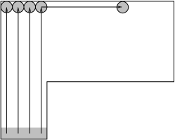
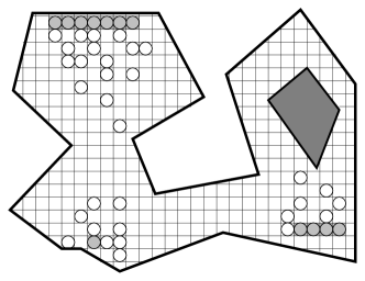
Figure 1: Left: One turn can cut off most of the flow lines leading out of the door pixels (shaded grey): The left three columns of robots are trapped. Right: A polygonal domain encloses a discrete set of possible robot locations (pixels); special door pixels are shown in grey.

1.1 Our Results

We develop and analyze algorithms for dispersing robot swarms in an unknown environment $R$. The primary objective is to minimize the makespan, that is, the time to fill the entire region. An environment is composed of squares or pixels that form a connected subset of the integer grid; such an environment is also called a maze. There is at most one robot per pixel and robots move horizontally or vertically at unit speed. There is a source of robots entering the environment through $k\geq 1$ doors. Robots are primitive finite automata, only having local communication, local sensors, and a constant-sized memory. The challenge is in proving that purely local strategies distributed over a swarm of agents can result in a predictable and provable behavior for the collective.

This paper presents the following results:

• We give filling algorithms for the single-door case (i.e., $k=1$), analyzing the algorithms both theoretically and experimentally in terms of natural performance metrics, such as makespan and total traveled distance by all robots. Our algorithms are based on leader-follower strategies that are adapted from depth-first and breadth-first search to apply to robot swarms. We prove that our algorithms have optimal makespan $2A-1$, where $A$ is the area (number of pixels) of $R$.

• We give a filling algorithm for the multi-door case ($k\geq 1$), also based on a leader-follower strategy. The emergent behavior of the swarm is a filling strategy, called laminar flow, that generalizes the “left-hand-on-wall” strategy to multiple streams of robots coming in through multiple doors. An important contribution of the algorithm is the formulation of splitting and splicing strategies that maintain a large flow of robots out of the doors. We prove that the laminar flow algorithm is $O(\log(k+1))$-competitive, that is, the ratio of the makespan of our algorithm to the optimal makespan is $O(\log(k+1))$.

• We give a matching lower bound of $\Omega(\log(k+1))$ on the competitiveness of the natural class of “simple-minded” strategies that use only strictly local information.

• We report on experiments with a Java simulator that we built for swarms in grid environments. All of the algorithms in this paper are implemented in this simulator.

While our results here are given purely in terms of robots moving synchronously on discrete grids, the results apply also to dispersing swarms of robots within an arbitrary connected planar domain, in the ideal setting in which the robots have perfect motion control and synchrony. More importantly, our results may form the foundation for theoretical work on more realistic models of swarm robotics in the continuum, with asynchronous motion, sensor errors, slippage, and hardware failures.

1.2 Prior and Related Work

There has been considerable study recently of distributed control and coordination of a set of autonomous robots. Gage [14, 15] has proposed the development of command and control tools for arbitrarily large swarms of microrobots and has proposed coverage paradigms in the context of robot dispersal in an environment. Payton et al [20, 21] propose the notion of “pheromone robotics” for world-embedded computation. Wagner et al. [9, 27, 28, 29] developed multi-robot algorithms, directly inspired by ant behaviors, for searching and covering. Principe et al [13, 22] and Suzuki et al [12, 25, 26] have studied algorithmic aspects of pattern formation in distributed autonomous robotics under various models of robots with minimal capabilities. The related flocking problem, which requires that a set of robots follow a leader while maintaining a formation, has been studied in several recent papers; see, e.g., [3, 6, 16]. Balch [2] has developed “Teambots”, a Java-based general-purpose multi-robot simulator.

There is a vast literature on algorithms for one or several robots to explore unknown environments. The environments can be modeled as graphs (directed or undirected), mazes, or geometric domains, and the robots can have a range of computing powers; see, e.g., [1, 7, 8, 10, 11]. Mitchell [19] includes a survey of many results on exploring and navigating in geometric environments.

Dispersion algorithms have been recently studied both in the context of multi-robot coverage and sensor network deployment; see [4, 5, 17, 30]. Methods include potential fields [17, 23], “artifical physics” [24], attraction-repulsion [18], and algorithms based on molecular dynamics [5]. While these studies have examined empirically the merits of heuristics, they have not addressed formally the algorithmic efficiency of the dispersion problem.

2 Preliminaries

For an arbitrary connected region ${\cal R}$ in the plane, we let $R$ denote the set of pixels that lie entirely within ${\cal R}$. A pixel is an axis-aligned unit square, $\{(x,y):i\leq x\leq i+1,j\leq y\leq j+1\}$, whose lower left corner is given by the integer grid point $(i,j)$. Two pixels are neighbors if they share a common edge; thus, pixel $(i,j)$ has four neighbors, $(i-1,j)$, $(i+1,j)$, $(i,j-1)$, and $(i,j+1)$. We refer to $R$ as the environment, and we assume that it is connected. A subset, $D\subset R$, of the pixels are doors, which serve as sources of incoming robots. See Figure 1(right).

A robot $r$ is said to occupy a pixel $p=(i,j)$ when it is located in that pixel. We assume that at most one robot can occupy any one pixel at any given time $t$. We let $p(r,t)$ denote the pixel occupied by robot $r$ at time $t$. We let $prev(r,t)=p(r,t-1)$ denote the pixel previously occupied by robot $r$.

Time is discretized into steps $t=0,1,2,3,\ldots$. The positions of the robots at time $t$ are given by the set $S(t)$, where $D\subseteq S(t)\subseteq R$. At time $0$, there is one robot in each door: $S(0)=D$.

Each pixel is in one of three states at time $t$: (1) the pixel is an obstacle if it does not lie in $R$; (2) the pixel is occupied if it is in $R$ and a robot occupies it; or (3) the pixel is unoccupied if it is in $R$ and no robot occupies it at time $t$. An unoccupied pixel at time $t$ is classified as either previously occupied, if it was occupied by some robot at some time prior to $t$, or frontier, if it has never been occupied.

Robots have sensors that detect information about the local environment. In particular, if a robot occupies pixel $(i,j)$ at time $t$, then we assume that it can detect the state of each pixel within a distance $r_{S}$ of $(i,j)$, where $r_{S}$ is the (fixed) sensor radius. Robots have no global sensor (e.g., a GPS) and no knowledge of the coordinates of the pixels they occupy.

We assume that each robot has a small finite memory that allows it to remember the sensor readings of the last $T\geq 1$ time steps; i.e., a robot knows the sensor readings it has taken at time $t-T$, $t-T+1,\ldots,t-1,t$. In particular, each robot knows which nearby pixels have been occupied recently by other robots. The algorithms in this paper have an $O(1)$-bit memory; thus, the robots have the computational power of finite automata.

We assume that robots have a limited ability to communicate with nearby robots. In particular, at any given time step a robot is able to exchange a constant-size message with any robot that lies within a prescribed communication radius, $r_{C}$, of the robot. The communication graph, ${\cal G}(t)$, of the swarm $S(t)$ at time $t$ is defined to be the undirected graph whose nodes are the robots $S(t)$ and whose edges link pairs of robots that communicate. The swarm is said to be connected at time $t$ if each connected component of ${\cal G}(t)$ contains at least one door pixel.

Robots move discretely on the grid of pixels. If at time $t$ a robot occupies pixel $(i,j)$ of $R$, and a neighboring pixel (say, $(i+1,j)\,$) of $R$ is unoccupied at time $t$, then the robot may take a step to the right, so that at time $t+1$ it occupies pixel $(i+1,j)$. Naturally, no two robots can move into the same pixel, since no pixel can be occupied by more than one robot. Thus, if two robots are occupying pixels that neighbor an empty pixel $p$ of $R$, then the robots must negotiate which one of them will have the right of way to enter $p$. A simple way to handle this negotiation is to establish a priority among the four directions, e.g., north, south, east, west. The robot occupying the pixel with the highest priority with respect to $p$ has first rights for moving to $p$.

The above rules on occupying and vacating pixels force a constant delay in the motion. Suppose that robot $r$ occupies pixel $(i,j)$ at time $t$ and vacates $(i,j)$ at time $t+1$. No other robot $r^{\prime}$ can occupy pixel $(i,j)$ during time $t+1$; the earliest possible time that the pixel can be occupied is $t+2$. In principal, we could vary these local rules. For example, we could allow robot $r^{\prime}$ to enter pixel $(i,j)$ at timestep $t+1$, if it enters in one direction while the current robot $r$ leaves in the opposite direction. However, these rules would require a much higher degree of coordination among the robots, and the movement decisions of robots would have to be less local. Specifically, whether a given robot can enter one pixel may depend on whether a different robot far away leaves another pixel. Alternatively, we could build a longer delay into the movement rules, but the resulting filling algorithms would be essentially the same. Note that the delay has an immediate impact on the necessary sensor range: If we require a delay of two time steps, robots need at least a sensor range of two, in order to be able to keep track of predecessors and successors.

A similar issue arises in the way new robots enter through the door. For simplicity, we assume that a door pixel is always occupied by a robot; as soon as the robot occupying a door pixel moves to an adjacent pixel, a new robot materializes at the door. One can consider there to be an infinite supply of robots on the “other side” of a door pixel, so that a new robot steps into the door whenever the robot that was there previously moves to another pixel of $R$. When a robot first appears at the door, we assume that the robot points north.

We say that the robots have filled the region $R$ at time $t$ if $S(t)=R$; in this case, the robots are well dispersed. A strategy is a set of rules by which robots move, basing their movement decisions solely on the constant amount of information they sense and remember. The makespan of a strategy is the minimum time, $t^{*}$, until the robots have filled the region $R$.

3 Dispersion Strategies for a Single Door

We begin with the case of a single door pixel $s$, which we call the source. We describe strategies based on the notion of “leaders” and “followers”.

A robot $r$ at time $t$ at position $p(r,t)$ is classified as moving (meaning that it is “active”) or stopped (meaning that it no longer moves). If $r$ is moving, it is classified as either a leader or a follower.

In our leader-follower strategies, each robot $r$ at time $t$ has a successor robot, $succ(r,t)$, that is following $r$ and a predecessor robot, $pred(r,t)$, that is leading $r$. If robot $r$ is at the door at time $t$ ($p(r,t)=s$), then we define $succ(r,t)$ to be NIL; if $r$ is a leader, then we define $pred(r,t)$ to be NIL.

At time $t=0$ there is a robot at the door $s$, which is designated as moving and as a leader.

3.1 Depth-First Leader-Follower

The depth-first leader-follower strategy (DFLF) is inspired by depth-first search in a graph. Specifically, at any given time $t\in\{0,1,2,3,\ldots\}$, there is exactly one leader, $r$, which is on pixel $p(r,t)$ and $r$ is looking for a frontier pixel (one that has never been occupied by a robot). (Thus, necessarily the pixel from which the robot came, $prev(r,t)$, is not frontier at time $t$.) If there are two or more frontier pixels neighboring $p(r,t)$, the leader selects any one of them as its next destination.

If the leader has no frontier pixel next to it, it stops (its state changes to “stopped”), and it tells its successor, $succ(r)$, to assume the leadership ($succ(r)$’s state changes to “leader”) at the conclusion of this time step. (The predecessor completes its move before taking over the leadership.) If the leader has no predecessor (i.e., it is a robot at the door), then the algorithm halts. (In this section, successors and (non-Nil) predecessors are invariant over time, and thus $t$ is removed from the argument.)

Any robot $r$ that is a follower (i.e., not the leader) simply follows its predecessor: at time $t$ it steps next to $prev(pred(r),t)$, the pixel previously occupied by the predecessor of $r$. Note that once a robot stops, it never moves again. Furthermore, at any point in time there is exactly one leader.

When dealing with finite automata, we have to use particular care when implementing the leader-follower strategy. As each robot has only a finite number of states, it cannot keep track of the identities of other robots, nor carry its own “ID label”. Instead, we use spatial information to pursue the immediate predecessor. Each robot $r$ has a “heading”, indicating the direction in which it is moving. The predecessor $pred(r)$ is the nearest robot in that direction. Similarly, each robot keeps track of its “tailing”, the direction from which it came. Thus, the successor is the nearest visible robot in that direction. Whenever a robot is about to change its heading, it signals this turn to its immediate successor. Heading and tailing are updated according to delay and sensor-range. This is reflected in the following lemma and corollary, which are proved by introduction on time.

Lemma 3.1.

If $r$ is not the leader at time $t$, then $prev(pred(r),t)$ is an unoccupied pixel neighboring $p(r,t)$. Furthermore, the maximum ($L_{1}$) distance between $r$ and $pred(r)$ is 2.

Corollary 3.2.

If a pixel is not occupied in two consecutive time steps $t$ and $t+1$, then it was never occupied before time $t$. (i.e., there are no “large gaps” of time in the occupation of a pixel.)

A further consequence of the above lemma and corollary is that the DFLF strategy can be implemented with a sensor radius of $r_{S}=2$ and a memory of $T=1$ (i.e., each robot recalls its previous sensor reading). Now it is not hard to derive the following result:

Theorem 3.3.

The DFLF algorithm halts when all pixels are occupied by robots. The makespan of the DFLF algorithm is $2A-1$, where $A$ is the number of pixels of the environment $R$.

Proof 3.4.

At each time step there is exactly one leader and that leader will do one of two things: (1) move to a frontier pixel, or (2) change its status to stopped and transfer leadership to its predecessor. (If the leader has no predecessor, that is, it is at the door, the algorithm halts.) Since each non-door pixel can be changed from frontier to non-frontier at most once, and each pixel can have a robot “park” itself on top of it at most once, the number of steps before the algorithm halts is at most $2A-1$. The algorithm does not stop earlier since there is always a leader and the leader must do one of the two actions ((1) or (2)) above.∎

Note that the factor 2 is a result of using a delay of 2. It is easy to see that this is best possible.

The total distance traveled by all robots in a filling using DFLF is at most $A^{2}$, since each robot steps at most $A$. We note that there are examples in which any dispersion strategy will require $\Omega(A^{2})$ total travel. One trivial example is a $1\times A$ rectangle, with the door pixel at one end. A trivial lower bound on the total travel for any given instance is the sum of the distances from each pixel of $R$ to the door.

DFLF may use substantially more total travel than an optimal (minimum makespan) strategy that minimizes total travel; consider, for example, a square with side lengths $A^{1/2}$, for which DFLF requires total travel of $A^{2}$ while an optimal strategy achieves total travel $O(A^{3/2})$.

3.2 Breadth-First Leader-Follower

We now describe an alternative dispersion algorithm, the breadth-first leader-follower (BFLF) strategy. BFLF often has advantages over the DFLF strategy in terms of other metrics of performance (total travel of the robots, maximum travel of any one robot, total relative distance, etc), while still being optimal in terms of makespan ($2A-1$).

The BFLF strategy is substantially more complex than the DFLF, as it is not trivial to implement breadth-first search with local decision rules on (finite-automata) robots; indeed, our strategy does not perform breadth-first search, but it “approximates” breadth-first search sufficiently well to have some similar properties.

As before, a robot can be in a “moving” state or a “stopped” state; however, we now introduce a third state, the waiting state, which is an interim state when a robot pauses temporarily and waits to be able to move. Once a robot is in a stopped state, it never moves again. In the BFLF strategy we can have multiple leaders, while in DFLF we have only one. As described for DFLF, we use a limited amount of spatial information to keep track of successors and predecessors. Other local rules are more complex and are described in the following.

Initially, there is one leader robot — the robot at the door, $s$. When a robot $r$ materializes at the door, it chooses to follow the previous robot that left the door. A leader always attempts to go to a neighboring frontier pixel, but makes sure it does not stray too far from its follower. If there are no neighboring frontier pixels, the leader waits for the immediate follower to catch up. As soon as the immediate follower catches up, the leader becomes stopped and passes on the leadership role to the immediate follower. If the leader $r$ at pixel $u$ has a choice among neighboring frontier pixels, it picks any one of them to be its heading. If other frontier pixels adjacent to $u$ remain unclaimed by other robots following different branches of dispersion, then the follower $r^{\prime}$ of $r$ will choose one of these pixels as its heading when it arrives at $u$; if there remains a frontier pixel adjacent to $u$, then $r^{\prime}$’s follower $r^{\prime\prime}$ chooses this pixel as its heading when it arrives at $u$. Here, $r^{\prime}$ and $r^{\prime\prime}$ are relabeled “leaders” and pixel $u$ is marked as a branching point.

A robot $r$ is only allowed to move at time $t$, if it satisfies the Movement Criterion (MC): A robot currently occupies $prev(r,t)$ (its “parent” position) or a robot is currently heading for $prev(r,t)$. If the MC is satisfied, the robot $r$ moves to its heading; otherwise, it remains at its current position, $p(r,t)$ but is still heading for its target pixel. As we will see below, a robot $r$ is never blocked by its immediate predecessor except for the time step at which $r$ first appears at the door or a time when its immediate predecessor is a leader with nowhere to go, meaning that the leadership will be passed to $r$.

The BFLF strategy tries to create as many paths as possible at all times. The visited pixels form a tree that guides the directions that robots move; thus, pixels have parents and grandparents. At branches in the tree (pixels with $\geq 2$ children), robots alternate the direction that they travel. Specifically, when a robot $r$ leaves a pixel at time $t$, it tells its immediate follower $r^{\prime}=succ(r,t)$ what $r^{\prime}$’s immediate destination should be. Branching enables robots arriving at the same pixel at different times to go in different directions, thereby balancing the flow.

Lemma 3.5.

If not all pixels are occupied, then some robot can move.

The following structural lemma shows that the BFLF algorithm is nonblocking, i.e., a robot $r$ is never “delayed” by its predecessors, only by its followers; i.e., only the MC holds a robot back, not temporary blockages downstream. Correctness follows by induction on the height of the tree.

Lemma 3.6.

If a robot is at pixel $v$ and a robot is at pixel $u$, the non-root parent of $v$, then the robot at $v$ is stopped.

Corollary 3.7.

A robot moves from the root every other time step, until all pixels are occupied. I.e., if a robot did not pop up at the root at time $t$, then one must pop up at time $t+1$, unless all pixels (including the root) are occupied.

Lemma 3.8.

The robots maintain a communication distance of $3$, meaning that the algorithm works for $r_{S}\geq 3$. The maximum $L_{1}$-distance from a robot to a follower is $3$. Furthermore, at least one of the following pixels is occupied when a robot is at pixel $u$: (1) the parent of $u$, (2) the grandparent of $u$, or (3) the uncle of $u$.

Putting all the claims together and using similar reasoning as for Theorem 3.3, we get the same kind of bound on the makespan:

Theorem 3.9.

The BFLF algorithm halts when all pixels are occupied by robots. The makespan of the BFLF algorithm is $2A-1$, where $A$ is the number of pixels of the environment $R$.

3.3 Experimental Comparison

While the DFLF and BFLF strategies both have optimal makespan, they differ with respect to other performance metrics. We have implemented in Java a simulator for testing our dispersion strategies, while measuring various performance measures, including: (1) the depth of the tree of all paths from the source (i.e., the length of the longest path of a robot); (2) the average distance traveled by a robot during the dispersion; and (3) the average of the ratios, $\rho_{i}=l_{i}/d_{i}$, of the ($L_{1}$) distance $l_{i}$ from the door to robot $i$’s final location to the total distance $d_{i}$ traveled by robot $i$ during the dispersion.

We have compared the DFLF and BFLF strategies for the case of a single door, in a variety of different environments. Our results show that the average depth of the tree grows substantially more rapidly, as a function of the number of pixels, for DFLF than it does for BFLF; e.g., for an $n$-by-$n$ square grid, BFLF tree depth grows linearly in $n$ while DFLF depth grows close to quadratically in $n$. Similarly, the average distance traveled by a robot using DFLF grows more rapidly than using BFLF. The average of the ratios $\rho_{i}=l_{i}/d_{i}$ decreases with increasing problem size for DFLF, while it increases for BFLF. Details of the experimental results are deferred to the full paper.

4 Dispersion with Multiple Doors

We now consider the case in which there are $k\geq 1$ door pixels. In order to achieve rapid filling, the objective is to maintain a flow of robots out of as many doors as possible. The difficulty is that one robot chain out of one door pixel may unnecessarily block the flow of robots out of other door pixels. (See the introduction and Figure 1(left) for examples.)

4.1 Laminar Flow Leader-Follower (LFLF) Algorithm

This section describes the Laminar Flow Leader-Follower (LFLF) algorithm. The LFLF algorithm maintains rapid flows by careful use of cutting and splicing. The emergent behavior of the swarm is a left-hand-on-wall strategy. The behavior of the algorithm is complex because bottlenecks in the environment may force the flow to divide into smaller flows that fill different regions and may merge and split.

In the LFLF algorithm there are $k$ multiple door pixels, $s_{1},s_{2},\cdots,s_{k}$. Note that LFLF matches DFLF algorithm if $k=1$. As in the $k=1$ case, our dispersion strategies are based on leaders and followers. A robot $r$ at time $t$ at position $p(r,t)$ is classified as active or inactive (stopped). If $r$ is active, it is either a leader or a follower. However, unlike for $k=1$, robots revert between leaders and followers. (In contrast, for $k=1$ a robot changes roles from follower to leader but only relinquishes the leader role by stopping and becoming inactive.) Furthermore, in DFLF once a robot stops, it becomes inactive. In contrast, in LFLF a robot may temporarily stop while still remaining active.

In LFLF (as in DFLF), robots have successors and predecessors, but in LFLF a robot’s immediate successor or predecessor may change over time. Thus, each robot $r$ at time $t$ has a predecessor robot denoted $\mbox{\em robot-pred}(r,t)$ and a successor robot denoted $\mbox{\em robot-succ}(r,t)$. If robot $r$ is at a door pixel at time $t$ ($p(r,t)=s_{i}$, for $i\in[1,k]$), then $\mbox{\em robot-succ}(r)=\mbox{NIL}$; if $r$ is a leader at time $t$, then $\mbox{\em robot-pred}(r)=\mbox{NIL}$.

Here we further refine the roles of the pixels. A pixel can be: (1) an obstacle, (2) a frontier pixel (a pixel that has never been occupied), (3) an inactive pixel, that is, an (occupied) pixel that hosts an inactive robot, (4) an active pixel, (which may be occupied or not). If a pixel is unoccupied but previously occupied, then it is always active; if a pixel is occupied, then it is active if and only if the robot it hosts is active.

Note that door pixels may be active or inactive, as described later. Active pixels play the role of transporting robots throughout the domain whereas inactive pixels are essentially obstacles. Analogous to the definition of predecessor and successor robots, each active pixel has predecessor and successor pixels. In particular, pixel $u$ at time step $t$ has successor pixel $\mbox{\em pixel-succ}(u,t)$ and predecessor pixel $\mbox{\em pixel-pred}(u,t)$. For door pixels $s_{i}$ at any time $t\geq 0$ $\mbox{\em pixel-succ}(u,t)=\mbox{NIL}$.

A leader pixel $u$ at time $t$ has $\mbox{\em pixel-pred}(u,t)=\mbox{NIL}$. As we will see, if a leader pixel contains a robot, then the robot is a leader, however the leader robot may not be on a leader pixel and the leader pixel may not contain robots. We call a chain of predecessor pixels starting from the door pixel $s_{i}$ and ending at a leader pixel, a flow line.

We now define formally the left side and right side of the flow. To do so, we first present some intermediate definitions. Consider a pixel $v$ at time $t$, and let $u=\mbox{\em pixel-succ}(v,t)$ and $w=\mbox{\em pixel-pred}(v,t)$. Let the incoming direction for $v$ at time $t$ be the vector $\overrightarrow{v\,u}$ and let the outgoing direction for $v$ at time $t$ be the vector $\overrightarrow{v\,w}$.

Consider the (vertical or horizontal) neighboring pixels, when we start from the incoming direction $\overrightarrow{v\,u}$ and rotate clockwise until reaching the outgoing direction $\overrightarrow{v\,w}$. Those neighboring pixels at intermediate (vertical or horizontal) orientations are defined to be on the left-hand side of $v$ time $t$. Thus, the left-hand side may contain $0$, $1$, or $2$ pixels. Any neighboring pixel that is not on the left-hand side, is on the right-hand side; this includes the pixels at the incoming and outgoing directions.

Note that leader pixels do not have outgoing edges, invalidating this definition. For a leader pixel, we define all neighboring pixels (except the successor pixel) to be on the left-hand side.

The left side of a flow line is the union of the left sides of the non-leader pixels in the flow line.

The essential idea the LFLF algorithm is to treat the left side of the flow line completely differently from the right side of the flow line. Specifically, we splice into the left-hand side but we cannot splice into the right.

4.2 Splicing and the LFLF Algorithm

Suppose that at time $t$ a leader robot $r_{a}$ reaches a pixel $u=p(r_{a},t)$. If $u$ has an (unoccupied) predecessor pixel $\mbox{\em pixel-pred}(u,t)$, then robot $r_{a}$ moves to this pixel. (Since $r_{a}$ is a leader robot, it will never have an occupied predecessor pixel.)

Otherwise, pixel $u=p(r_{a},t)$ is a leader pixel. If $u=p(r_{a},t)$ has no neighboring frontier pixels, then robot $r_{a}$ tries to pass on the leadership. Robot $r_{a}$ first looks for a neighboring active pixel $v$. If no such $v$ exists, then $r_{a}$ becomes inactive and passes the leadership to its successor robot $\mbox{\em robot-succ}(r_{a},t)$. When $r_{a}$ becomes inactive, pixel $u$ also becomes inactive and its successor pixel becomes the new leader pixel.

If robot $r_{a}$ looks for a neighboring active pixel $v$, and such a $v$ exists, then $r_{a}$ checks whether $u=p(r_{a},t)$ is a left-hand neighbor of $v$. If this is not the case for any possible $v$, then again $r_{a}$ becomes inactive and passes the leadership to its successor robot $\mbox{\em robot-succ}(r_{a},t)$. As before, when $r_{a}$ becomes inactive, pixel $u$ also becomes inactive and its successor pixel becomes the new leader pixel.

If there exists such a $v$, robot $r_{a}$ chooses the first such $v$ sweeping clockwise, starting from the incoming direction. We redefine the predecessor pixel $\mbox{\em pixel-pred}(u,t+1):=v$ and thus successor pixel $\mbox{\em pixel-succ}(v,t+1):=u$. Thus, the previous successor pixel of $v$ becomes a new leader pixel. (Note that this new leader pixel may or may not have a robot on it.) Now $r_{a}$ identifies its new leader; it follows predecessor pixels starting at $v$ until it finds a robot $r_{b}$ and sets $\mbox{\em robot-pred}(r_{a},t+1)=r_{b}$ and $\mbox{\em robot-succ}(r_{b},t+1)=r_{a}$. Robot $r_{a}$ then passes the leadership to $r_{c}=\mbox{\em robot-succ}(r_{b},t)$.

Figure 2: The LFLF algorithm: There are six door pixels in the lower left corner. Splicing enables the flow to turn a corner.

4.3 Correctness of LFLF

We now show that LFLF always fills an environment. During LFLF, we claim that the following invariant is maintained: The left side of a flow line consists of visited pixels and obstacles. This follows from the fact that, whenever a robot enters a pixel, it turns as far left as it can (left-hand-on-the-wall). The invariant implies the following lemma, which we use to show that the visited regions propagate out from obstacle pixels:

Lemma 4.1.

The union of boundary points separates the visited region from obstacles and the right side of flows. In other words, the unvisited region only touches a flow from its right.

Another useful property of flow lines is the following:

Lemma 4.2.

Flows do not self-intersect.

Lemma 4.3.

Leadership passing does not change the total number of leader robots. Thus, the number of leader robots at any time step $t$ is equal to the number of active doors.

Theorem 4.4.

The robots always fill environment $R$.

Proof 4.5.

When a robot becomes inactive, it is a leader and its surrounding pixels must all not be frontier, for otherwise $r$ would advance to such a pixel and still be active. Therefore, if an active pixel $u$ is next to a frontier pixel $v$, any robot advancing into $u$ will not become inactive and some flow lines can advance into the empty region so it will be filled.∎

In the next sections we analyze the makespan for this filling strategy.

4.4 Competitive Analysis for Online Strategies

For any strategy ${\cal S}$, let $n_{\cal S}(t)$ be the number of robots that enter through the doors during timestep $t$; we define $n_{\cal S}(0)=k$.

Note that the inherent delay of $2$ in robot movement means that $n_{\cal S}(t)$ is a highly erratic function, so that in one timestep $k$ robots might enter the doors, implying that in the next timestep no robots enter the doors. In LFLF additional delays are caused by splicings, and therefore we cannot even say that a robot enters an active door pixel every other timestep. To understand why, consider Figure 2. When one flow line splices into a different flow line, a robot may get delayed by one additional time step in order to obtain the required separation between robots. If many splicing are happening next to each other, this can cause an accumulated delay of up to $k$ time units, which causes a “wave” of packed robots that propagates back towards the door pixels. Thus, a door pixel might temporarily hold off ejecting robots for many units without the door pixel becoming inactive. Whenever an active door pixel does not eject a robot we say there is a door-pixel delay.

Fortunately, the following lemma bounds the number of splicings (and also the total number of door-pixel delays).

Lemma 4.6.

A pixel can only be used to initiate $O(1)$ splicings.

Theorem 4.7.

The LFLF strategy is $O(\log(k+1))$-competitive.

Proof 4.8.

Consider the times $\{t_{i}\}_{i=0}^{\lceil\log(k+1)\rceil}$, where $t_{i}$ is the latest timestep during which at least $k/2^{i}$ door pixels are active. We call times $t_{0},t_{1},t_{2},\ldots,t_{\lceil\log(k+1)\rceil}$ significant events. Consider the time interval from $t_{i}$ to $t_{i+1}$, when at least $k/2^{i+1}$ door pixels are active. Thus, the total number of robots leaving the door plus door-pixel delays during this interval is at least $(k/2^{i+1})(t_{i+1}-t_{i})$.

Now consider an optimal strategy ${\cal S}^{*}$, and consider the cut $\chi$ associated with the significant event $t_{i}$ of LFLF. Cut $\chi$ is the boundary between the occupied and frontier pixels and has size at most $k/2^{i}$. A lower bound on the makespan of any strategy is the area “behind” $\chi$ (i.e., the side of $\chi$ not containing the doors) divided by the length of $\chi$ plus the amount of time required to send the flow from the door to reach $\chi$. Thus, the makespan, opt, of ${\cal S}^{*}$ satisfies

$$\mbox{\sc opt}\geq\frac{{k}/{2^{i+1}}(t_{i+1}-t_{i})}{{k}/{2^{i}}}=(t_{i+1}-t_{i})/2.$$

Summing over all significant events we obtain that the total filling time of LFLF is $O(\mbox{\sc opt}\cdot\log(k+1))$.∎

If we disregard the issue of delays caused by pixels having to be fully vacated before being re-entered, we get a whole class called sensible strategies, defined by the following two conditions:

(1)

$n_{\cal S}(t)$ is non-increasing in $t$; and

(2)

If $n_{\cal S}(t)>n_{\cal S}(t+1)$, then at time $t$ the number of occupied pixels bordering on a frontier pixel is $n_{\cal S}(t+1)$.

The above proof also implies the following; quite clearly, this result still holds if we extend the notion of sensible strategies to allow for some delays, as long as these only add a constant factor to the filling times.

Theorem 4.9.

Any sensible strategy is $O(\log(\frac{k}{b}+1))$-competitive.

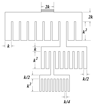
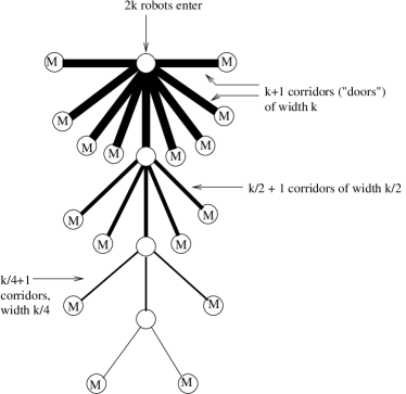
Figure 3: Left: An environment that is hard for both depth-first and breadth-first filling strategies. This example shows that LFLF and related strategies are $\Omega(\log(k+1))$ competitive. Right: A scenario in which any simple-minded strategy is $\Omega(\log(k+1))$ competitive.

4.5 Competitive Analysis of Simple-Minded Strategies

Under certain natural assumptions that limit the power of strategies, it is possible to give matching lower bounds on the competitiveness. To give some intuition, consider first the class of examples shown in Figure 3(left), which shows that the laminar flow algorithm may take as much as $\Omega(\log(k+1))$ times opt.

Theorem 4.10.

The LFLF algorithm is $\Omega(\log(k+1))$-competitive.

This lower bound can be generalized to a much larger class of strategies. We say that strategy ${\cal S}$ is simple-minded if the following condition holds: There is a constant $C$, such that we can only tell the number $A^{\prime}$ of pixels in a region $R^{\prime}\subseteq R$ when a set $R^{\prime\prime}\subseteq R$ has been visited that has all pixels in $R^{\prime}$ within $L_{1}$ distance $C$.

Considering simple-minded strategies is quite natural in the context of robot swarms: If we assume we only “know” a region $R^{\prime}$ after each pixel has been seen by one of the robots, then the constant $C$ corresponds precisely to the sensor range. The example of Figure 3(left) can be generalized as shown schematically in Figure 3(right), which forms the basis for the proof of the following theorem:

Theorem 4.11.

Any simple-minded strategy is $\Omega(\log(k+1))$-competitive.

A particular subclass of simple-minded strategies is one that arises quite naturally in exploration problems: We say that a strategy is conservative if any pixel that has been “discovered”, i.e., come within sensor range of a robot, must stay within sensor range of some robot. For a constant-size sensor range, it is easy to prove the following statement, which has been claimed for a long time in a different context:

Proposition 4.12.

All conservative strategies are simple-minded.

As the LFLF strategy is conservative by design, we conclude that the lower bound of Theorem 4.11 applies to LFLF.

Acknowledgements

We thank N. Jovanovic and M. Sztainberg for contributions to this research. This reseearch was partially supported by HRL Labs (a DARPA subcontract), Honda Fundamental Research Labs, NASA Ames Research (NAG2-1325), NSF (CCR-0098172, EIA-0112849, CCR-0208670), U.S.-Israel Binational Science Foundation, and Sandia National Labs.

References

- [1] B. Awerbuch, M. Betke, R. L. Rivest, and M. Singh. Piecemeal graph exploration by a mobile robot. In Proc. 8th Annual ACM Conference on Computational Learning Theory, pages 321–328, 1995.
- [2] T. Balch. http://www.teambots.org.
- [3] T. Balch and R. C. Arkin. Behavior-based formation control for multi-robot teams. IEEE Transactions on Robotics and Automation, 14(6):926–939, 1998.
- [4] M. A. Batalin and G. S. Sukhatme. Multi-robot dynamic coverage of a planar bounded environment. Technical report, Robotic Embedded Systems Laboratory, University of Southern California, 2002.
- [5] M. A. Batalin and G. S. Sukhatme. Spreading out: A local approach to multi-robot coverage. In H. Asama, T. Arai, T. Fukuda, and T. Hasegawa, editors, Proc. 6th International Symposium on Distributed Autonomous Robotic Systems, Fukuoka, Japan, 2002. Springer-Verlag.
- [6] O. B. Bayazit, J.-M. Lien, and N. M. Amato. Better flocking behaviors using rule-based roadmaps. In Proc. 5th International Workshop on Algorithmic Foundations of Robotics, 2002.
- [7] M. A. Bender, A. Fernández, D. Ron, A. Sahai, and S. Vadhan. The power of a pebble: Exploring and mapping directed graphs. Information and Computation, 176:1–21, 2002.
- [8] M. A. Bender and D. Slonim. The power of team exploration: Two robots can learn unlabeled directed graphs. In Proc. 35th Annual Symposium on Foundations of Computer Science, pages 75–85, 1994.
- [9] A. M. Bruckstein, C. L. Mallows, and I. A. Wagner. Probabilistic pursuits on the grid. American Mathematical Monthly, 104(4):323–343, 1997.
- [10] X. Deng and C. H. Papadimitriou. Exploring an unknown graph. In Proc. 31st Annual Symposium on Foundations of Computer Science, pages 356–361, 1990.
- [11] G. Dudek, M. Jenkin, E. Milios, and D. Wilkes. Map validation and robot self-location in a graph-like world. Robotics and Autonomous Systems, 22(2):159–178, 1997.
- [12] A. Dumitrescu, I. Suzuki, and M. Yamashita. High speed formations of reconfigurable modular robotic systems. In Proc. IEEE International Conference on Robotics and Automation (ICRA ’02), pages 123–128, 2002.
- [13] P. Flocchini, G. Prencipe, N. Santoro, and P. Widmayer. Distributed coordination of a set of autonomous mobile robots. In Proc. IEEE Intelligent Vehicle Symposium (IV 2000), pages 480–485, 2000.
-
[14]
D. Gage.
Many-robot systems.
http://www.spawar.navy.mil/robots/research/manyrobo/manyrobo.html. - [15] D. Gage. Sensor abstractions to support many-robot systems. In Proc. of SPIE Mobile Robots VII, Boston MA, 1992, Vol. 1831, pages 235–246, 1992.
- [16] V. Gervasi and G. Prencipe. Flocking by a set of autonomous mobile robots. Technical Report TR-01-24, University of Pisa, Oct. 2001.
- [17] A. Howard, M. J. Mataric, and G. S. Sukhatme. Mobile sensor network deployment using potential fields: A distributed scalable solution to the area coverage problem. In H. Asama, T. Arai, T. Fukuda, and T. Hasegawa, editors, Proc. 6th International Symposium on Distributed Autonomous Robotic Systems, Fukuoka, Japan, 2002. Springer-Verlag.
- [18] T-R. Hsiang, N. Jovanovic, and M. Sztainberg. Dispersion Protocols for Robot Swarms. Technical Report, Stony Brook University, 2002.
- [19] J. S. B. Mitchell, Geometric shortest paths and network optimization, In Handbook of Computational Geometry (J.-R. Sack and J. Urrutia, editors), pages 633–701. Elsevier Science Publishers B.V. North-Holland, Amsterdam, 2000.
- [20] D. Payton, R. Estkowski, M. Howard. Progress in Pheromone Robotics. In Proc. 7th International Conference on Intelligent Autonomous Systems, 2002.
- [21] D. Payton, M. Daily, R. Estkowski, M. Howard, C. Lee. Pheromone Robotics. Autonomous Robots, Vol. 11, No. 3, pages 319-324, 2001.
-
[22]
G. Prencipe.
Distributed Coordination of a Set of Autonomous Mobile Robots.
Ph.D. thesis Dipartimento di Informatica, Università degli Studi di Pisa, 2002.
http://www.di.unipi.it/phd/tesi/tesi_2002/PhDthesis_Prencipe.ps.gz. - [23] J. H. Reif and H. Wang. Social potential fields: A distributed behavioral control for autonomous robots. Robotics and Autonomous Systems, 27(3):171–194, 1999.
- [24] W. Spears and D. Gordon. Using artificial physics to control agents. In Proc. IEEE Internat. Conf. on Information, Intelligence, and Systems, 1999.
- [25] K. Sugihara and I. Suzuki. Distributed algorithms for formation of geometric patterns with many mobile robots. Journal of Robotic Systems, 13(3):127–139, 1996.
- [26] I. Suzuki and M. Yamashita. Distributed anonymous mobile robots: Formation of geometric patterns. SIAM Journal on Computing, 28(4):1347–1363, 1999.
- [27] I. Wagner and A. Bruckstein. Cooperative cleaners: a study in ant robotics. Technical Report CIS9512, Technion, 1995.
- [28] I. Wagner, M. Lindenbaum, and A. Bruckstein. Distributed covering by ant-robots using evaporating traces. IEEE Transactions on Robotics and Automation, 15(5):918–933, 1999.
- [29] I. A. Wagner, M. Lindenbaum, and A. M. Bruckstein. Efficiently searching a graph by a smell-oriented vertex process. Annals of Mathematics and Artificial Intelligence, 24(1-4):211–223, 1998.
- [30] A. Winfield. Distributed sensing and data collection via broken ad hoc wireless connected networks of mobile robots. In L.E. Parker, G.W. Bekey, and J. Barhen, editors, Distributed Autonomous Robotic Systems, Vol. 4, pp. 273–282, 2000. Springer-Verlag.