Approximating Incomplete Kernel Matrices by the em Algorithm

Abstract

In biological data, it is often the case that observed data are available only for a subset of samples. When a kernel matrix is derived from such data, we have to leave the entries for unavailable samples as missing. In this paper, we make use of a parametric model of kernel matrices, and estimate missing entries by fitting the model to existing entries. The parametric model is created as a set of spectral variants of a complete kernel matrix derived from another information source. For model fitting, we adopt the em algorithm based on the information geometry of positive definite matrices. We will report promising results on bacteria clustering experiments using two marker sequences: 16S and gyrB.

1 Introduction

In kernel machines such as support vector machines (SVM) (Schölkopf and Smola, 2001), objects are represented as a kernel matrix, where $n$ objects are represented as an $n\times n$ positive semidefinite matrix. Essentially the $(i,j)$ entry of the kernel matrix describes the similarity between $i$-th and $j$-th objects. Due to positive semidefiniteness, the objects can be embedded as $n$ points in an Euclidean feature space such that the inner product between two points equals to the corresponding entry of kernel matrix. This property enables us to apply diverse learning methods (for example, SVM or kernel PCA) without explicitly constructing a feature space (Schölkopf and Smola, 2001).

Biological data such as amino acid sequences, gene expression arrays and phylogenetic profiles are derived from expensive experiments (Brown, 1999). Typically initial experimental measurements are so noisy that they cannot be given to learning machines directly. Since high quality data are created by extensive work of human experts, it is often the case that good data are available only for a subset of samples. When a kernel matrix is derived from such incomplete data, we have to leave the entries for unavailable samples as missing. We call such a matrix an “incomplete matrix”. Our aim is to estimate the missing entries, but it is obviously impossible without additional information. So we make use of a parametric model of admissible matrices, and estimate missing entries by fitting the model to existing entries.

In this scheme, it is important to define a parametric model appropriately. For example, Graepel (2002) used the set of all positive definite matrices as a model. Although this model worked well when only a few entries are missing, this model is too general for our cases where whole columns and rows are missing. Thus we need another information source for constructing a parametric model. Fortunately, in biological data, it is common that one object is described by two or more representations. For example, genes are represented by gene networks and gene expression arrays at the same time (Vert and Kanehisa, 2002). Also a bacterium is represented by several marker sequences (Yamamoto et al., 2000). In this paper, we assume that a complete matrix is available from another information source, and a parametric model is created by giving perturbations to the matrix. We call the complete matrix a “base matrix”. When creating a parametic model of admissible matrices from a base matrix, one typical way is to define the parametric model as all spectral variants of the base matrix, which have the same eigenvectors but different eigenvalues (Cristianini et al., 2002). When several base matrices are available, the weighted sum of these matrices would be a good parametric model as well (Lanckriet et al., 2002).

In order to fit a parametric model, the distance between two matrices has to be determined. A common way is to define the Euclidean distance between matrices (for example, the Frobeneous norm) and make use of the Euclidean geometry. Recently Vert and Kanehisa (2002) tackled with the incomplete matrix approximation problem by means of kernel CCA. Also Cristianini et al. (2002) proposed a similarity measure called “alignment”, which is basically the cosine between two matrices. In contrast that their methods are based on the Euclidean geometry, this paper will follow an alternative way: we will define the Kullback-Leibler (KL) divergence between two kernel matrices and make use of the Riemannian information geometry (Ohara et al., 1996). The KL divergence is derived by relating a kernel matrix to a covariance matrix of Gaussian distribution. The primal advantage is that the KL divergence allows us to use the $em$ algorithm (Amari, 1995) to approximate an incomplete kernel matrix. The $e$ and $m$ steps are formulated as convex programming problems, and moreover they can be solved analytically when spectral variants are used as a parametric model.

We performed bacteria clustering experiments using two marker sequences: 16S and gyrB (Yamamoto et al., 2000). We derived the incomplete and base kernel matrices from gyrB and 16S, respectively. As a result, even when 50% of columns/rows are missing, the clustering performance of the completed matrix was better than that of the base matrix, which illustrates the effectiveness of our approach in real world problems.

This paper is organized as follows: Sec. 2 introduces the information geometry to the space of positive definite matrices. Based on geometric concepts, the em algorithm for matrix approximation is presented in Sec. 3, where detailed computations are deferred in Sec. 4. In Sec. 5, the matrix approximation problem is formulated as statistical inference and the equivalence between the em and EM algorithms (Dempster et al., 1977) is shown. Then the bacteria clustering experiment is described in Sec. 6. After seeking for possible extensions in Sec. 7, we conclude the paper in Sec. 8.

2 Information Geometry of Positive Definite Matrices

We first explain how to introduce the information geometry in the space of positive definite matrices. Only necessary parts of the theory will be presented here, so refer to (Ohara et al., 1996; Amari and Nagaoka, 2001) for details.

Let us define the set of all $d\times d$ positive definite matrices as ${\cal P}$. The first step is to relate a $d\times d$ positive definite matrix $P\in{\cal P}$ to the Gaussian distribution with mean 0 and covariance matrix $P$:

$$p({\boldsymbol{x}}|P)=\frac{1}{(2\pi)^{d/2}|P|^{1/2}}\exp(-\frac{1}{2}{\boldsymbol{x}}^{\top}P^{-1}{\boldsymbol{x}}).$$ (1)

It is well known that the Gaussian distribution belongs to the exponential family. The canonical form of an exponential family distribution is written as

$$p({\boldsymbol{x}}|{\boldsymbol{\theta}})=\exp({\boldsymbol{\theta}}^{\top}{\boldsymbol{r}}({\boldsymbol{x}})-\psi({\boldsymbol{\theta}})),$$

where ${\boldsymbol{r}}({\boldsymbol{x}})$ is the vector of sufficient statistics, ${\boldsymbol{\theta}}$ is the natural parameter and $\psi({\boldsymbol{\theta}})$ is the normalization factor. When (1) is rewritten in the canonical form, we have the sufficient statistics as

$${\boldsymbol{r}}({\boldsymbol{x}})=-\left(\frac{1}{2}x_{1}^{2},\ldots,\frac{1}{2}x_{d}^{2},x_{1}x_{2},\ldots,x_{d-1}x_{d}\right)^{\top},$$

and the natural parameter as

$${\boldsymbol{\theta}}=\left([P^{-1}]_{11},\ldots,[P^{-1}]_{dd},[P^{-1}]_{12},\ldots,[P^{-1}]_{d-1,d}\right)^{\top},$$

where $[M]_{ij}$ denotes the $(i,j)$ entry of matrix $M$. The natural parameter ${\boldsymbol{\theta}}$ provides a coordinate system to specify a positive definite matrix $P$, which is called the ${\boldsymbol{\theta}}$-coordinate system (or the $e$-coordinate system). On the other hand, there is an alternative representation for the exponential family. Let us define the mean of $r_{i}(x)$ as $\eta_{i}$: For example, when $r_{i}(x)=x_{s}x_{t}$,

$$\eta_{i}=\int x_{s}x_{t}p({\boldsymbol{x}}|{\boldsymbol{\theta}})d{\boldsymbol{x}}=P_{st}.$$

This new set of parameters $\eta_{i}$ provides another coorninate system, called ${\boldsymbol{\eta}}$-coordinate system (or the $m$-coordinate system):

$${\boldsymbol{\eta}}=\left(P_{11},\ldots,P_{dd},P_{12},\ldots,P_{d-1,d}\right)^{\top}.$$

Let us consider the following curve ${\boldsymbol{\theta}}(t)$ connecting two points ${\boldsymbol{\theta}}_{1}$ and ${\boldsymbol{\theta}}_{2}$ linearly in ${\boldsymbol{\theta}}$ coordinates:

$${\boldsymbol{\theta}}(t)=t({\boldsymbol{\theta}}_{2}-{\boldsymbol{\theta}}_{1})+{\boldsymbol{\theta}}_{1}.$$

When written is the matrix form, this reads

$$P^{-1}(t)=t(P^{-1}_{2}-P^{-1}_{1})+P^{-1}_{1}.$$

This curve is regarded as a straight line from the exponential viewpoint and is called an exponential geodesic or $e$-geodesic. In particular, each coordinate curve $\theta_{i}=t$, $\theta_{j}=c_{j}~{}~{}(j\neq i)$ is an $e$-geodesic. When the $e$-geodesic between any two points in a manifold ${\cal S}\subseteq{\cal P}$ is included in ${\cal S}$, the manifold ${\cal S}$ is said to be $e$-flat. On the other hand, the mixture geodesic or $m$-geodesic is defined as

$${\boldsymbol{\eta}}(t)=t({\boldsymbol{\eta}}_{2}-{\boldsymbol{\eta}}_{1})+{\boldsymbol{\eta}}_{1}.$$

In the matrix form, this reads

$$P(t)=t(P_{2}-P_{1})+P_{1}.$$

When the $m$-geodesic between any two points in ${\cal S}$ is included in ${\cal S}$, the manifold ${\cal S}$ is said to be $m$-flat.

In information geometry, the distance between probability distributions is defined as the Kullback-Leibler divergence (Amari and Nagaoka, 2001):

$$KL(p,q)=\int p(x)\log\frac{p(x)}{q(x)}dx.$$

By relating a positive definite matrix to the covariance matrix of Gaussian (1), we have the Kullback-Leibler (KL) divergence for two matrices $P,Q$:

$$KL(P,Q)=\operatorname{tr}(Q^{-1}P)+\log\det Q-\log\det P-d.$$

With respect to a manifold ${\cal S}\subseteq{\cal P}$ and a point $P\in{\cal P}$, the projection from $P$ to ${\cal S}$ is defined as the point in ${\cal S}$ closest to $P$. Since the KL divergence is asymmetric, there are two kinds of projection:

• $e$-projection: $Q^{*}=\operatorname{argmin}_{Q\in{\cal S}}KL(Q,P)$.

• $m$-projection: $Q^{*}=\operatorname{argmin}_{Q\in{\cal S}}KL(P,Q)$.

It is proved that the $m$-projection to an $e$-flat submanifold is unique, and $e$-projection to an $m$-flat manifold is unique (Amari and Nagaoka, 2001). This uniqueness property means that the corresponding optimization problem is convex and so the global optimal solution is easily obtained by any reasonable method.

3 Approximating an Incomplete Kernel Matrix

In this section, we describe the em algorithm to approximate an incomplete kernel matrix. Let $x_{1},\ldots,x_{\ell}\in{\cal X}$ be the set of samples in interest. In supervised learning cases, this set includes both training and test sets, thus we are considering the transductive setting (Vapnik, 1998). Let us assume that the data is available for the first $n$ samples, and unavailable for the remaining $m:=\ell-n$ samples. Denote by $K_{I}$ an $n\times n$ kernel matrix, which is derived from the data for the first $n$ samples. Then, an incomplete kernel matrix is described as

$$D=\left(\begin{array}[]{cc}K_{I}&D_{vh}\\ D_{vh}^{\top}&D_{hh}\end{array}\right),$$ (2)

where $D_{vh}$ is an $n\times m$ matrix and $D_{hh}$ is an $m\times m$ symmetric matrix. Since $D$ has missing entries, it cannot be presented as a point in ${\cal P}$. Instead, all the possible kernel matrices form a manifold

$${\cal D}=\{D\;|\;D_{vh}\in\Re^{n\times m},\;\;D_{hh}\in\Re^{m\times m},\;\;D_{hh}=D_{hh}^{\top},\;\;D\succ 0\},$$

where $D\succ 0$ means that $D$ is positive definite. We call it the data manifold as in the conventional EM algorithm (Ikeda et al., 1999). It is easy to verify that $\cal D$ is an $m$-flat manifold; hence, the $e$-projection to $\cal D$ is unique.

Next let us define the parametric model to approximate $D$. Here the model is derived as the spectral variants of $K_{B}$, which is an $\ell\times\ell$ base kernel matrix derived from another information source. Let us decompose $K_{B}$ as

$$K_{B}=\sum_{i=1}^{\ell}\lambda_{i}{\boldsymbol{v}}_{i}{\boldsymbol{v}}_{i}^{\top},$$

where $\lambda_{i}$ and ${\boldsymbol{v}}_{i}$ is the $i$-th eigenvalue and eigenvector, respectively. Define

$$M_{i}={\boldsymbol{v}}_{i}{\boldsymbol{v}}_{i}^{\top},$$ (3)

then all the spectral variants are represented as

$${\cal M}=\{M\;|\;M=\sum_{j=1}^{\ell}\beta_{j}M_{j},\;\;{\boldsymbol{\beta}}\in\Re^{\ell},\;\;M\succ 0\}$$

We call it the model manifold (Ikeda et al., 1999). For notational simplicity, we choose a different parametrization of ${\cal M}$:

$${\cal M}=\{M\;|\;M=(\sum_{j=1}^{\ell}b_{j}M_{j})^{-1},\;\;{\boldsymbol{b}}\in\Re^{\ell},\;\;M\succ 0\},$$ (4)

where $b_{j}=1/\beta_{j}$. It is easily seen that the manifold ${\cal M}$ is $e$-flat and $m$-flat at the same time. Such a manifold is called dually-flat.

Our approximation problem is formulated as finding the nearest points in two manifolds: Find $D\in{\cal D}$ and $M\in{\cal M}$ to minimize $KL(D,M)$. In geometric terms, this problem is to find the nearest points between $e$-flat and $m$-flat manifolds. It is well known that such a problem is solved by an alternating procedure called the em algorithm (Amari, 1995). The em algorithm gradually minimizes the KL divergence by repeating $e$-step and $m$-step alternately (Fig. 1).

\psfrag{ddd}{${\cal D}$}\psfrag{mmm}{${\cal M}$}\includegraphics[width=216.81pt]{em.eps}

Figure 1: Information geometric picture of the $em$ algorithm. The data manifold ${\cal D}$ corresponds to the set of all completed matrices, whereas the model manifold ${\cal M}$ corresponds to the set of all spectral variants of a base matrix. The nearest points are found by gradually minimizing the KL divergence by repeating $e$ and $m$ projections.

In the $e$-step, the following optimization problem is solved with fixing $M$: Find $D\in{\cal D}$ that minimizes $KL(D,M)$. This is rewritten as follows: Find $D_{vh}$ and $D_{hh}$ that minimize

$$L_{e}=\operatorname{tr}(DM^{-1})-\log\det D,$$ (5)

subject to the constraint that $D\succ 0$. Notice that this constraint is not needed, because

$$\log\det D=\sum_{i=1}^{\ell}\log\mu_{i},$$

where $\mu_{i}$ is the $i$-th eigenvalue of $D$. Here $\log\det D$ is undefined when one of eigenvalues is negative, and $\log\det D$ decreases to $-\infty$ as an eigenvalue get closer to 0. So, at the optimal solution, $D$ is necessarily positive definite, because the KL divergence is infinite otherwise. As indicated by information geometry, this is a convex problem, which can readily be solved by any reasonable optimizer. Moreover the solution is obtained in a closed form: Let us partition $M^{-1}$ as

$$M^{-1}=\left(\begin{array}[]{cc}S_{vv}&S_{vh}\\ S_{vh}^{\top}&S_{hh}\end{array}\right).$$ (6)

The solution of (5) is described as

$$D_{vh} = -K_{I}S_{vh}S_{hh}^{-1},$$ (7)

$$D_{hh} = S_{hh}^{-1}+S_{hh}^{-1}S_{vh}K_{I}S_{vh}S_{hh}^{-1}.$$ (8)

The derivation of (7) and (8) will be described in Sec. 4.1.

In the $m$-step, the following optimization problem is solved with fixing $D$: Find $M\in{\cal M}$ that minimizes $KL(D,M)$. This is rewritten as follows: Find ${\boldsymbol{b}}\in\Re^{\ell}$ that minimizes

$$L_{m}=\sum_{j=1}^{\ell}b_{j}\operatorname{tr}(M_{j}D)-\log\det(\sum_{j=1}^{\ell}b_{j}M_{j})$$ (9)

subject to the constraint that $\sum_{j=1}^{\ell}b_{j}M_{j}\succ 0$. Notice that this constraint can be ignored as well. When $\{M_{j}\}_{j=1}^{\ell}$ are defined as (3), the closed form solution of (9) is obtained as

$$b_{i}=1/\operatorname{tr}(M_{i}D),\qquad i=1,\ldots,\ell.$$ (10)

The derivation of (10) will be described in Sec. 4.2.

4 Computing Projections

This section presents the derivation of $e$ and $m$-projections in detail.

4.1 $e$-projection

First we will show the derivation of $e$-projection (7) and (8). The log determinant of a partitioned matrix is rewritten as

$$L_{e} = \operatorname{tr}(DM^{-1})-\log\det D$$

$$= \operatorname{tr}(DM^{-1})-\log\det K_{I}-\log\det(D_{hh}-D_{vh}^{\top}K_{I}^{-1}D_{vh}).$$

When we partition $M^{-1}$ as (6), it turns out that

$$L_{e}=\operatorname{tr}(D_{vv}S_{vv})+2\operatorname{tr}(D_{vh}S_{vh})+\operatorname{tr}(D_{hh}S_{hh})-\log\det K_{I}-\log\det(D_{hh}-D_{vh}^{\top}K_{I}^{-1}D_{vh}).$$ (11)

The saddle point equation with respect to $D_{hh}$ is obtained as

$$\frac{\partial L_{e}}{\partial D_{hh}}=S_{hh}-(D_{hh}-D_{vh}^{\top}K_{I}^{-1}D_{vh})^{-1},$$ (12)

because $\frac{\partial}{\partial C}\log\det C=C^{-1}$ for any symmetric matrix $C$. Solving (12) with respect to $D_{hh}$, we have

$$D_{hh}=S_{hh}^{-1}+D_{vh}^{\top}K_{I}^{-1}D_{vh}.$$ (13)

Substituting (13) into (11), we have

$$L_{e}=\operatorname{tr}(D_{vv}S_{vv})+2\operatorname{tr}(D_{vh}S_{vh})+\operatorname{tr}(I+S_{hh}D_{vh}^{\top}K_{I}^{-1}D_{vh})-\log\det K_{I}-\log\det S_{hh}.$$

Now the saddle point equation with respect to $D_{vh}$ is obtained as

$$\frac{\partial L_{e}}{\partial D_{vh}}=2S_{vh}+2K_{I}^{-1}D_{vh}S_{hh}=0.$$

Solving this equation, we have the solution (7) for $D_{vh}$. By substituting (7) into (13), we have the solution (8) for $D_{hh}$.

4.2 $m$-projection

Next, we will show the derivation of $m$-projection (10). The $m$ projection is obtained as the solution ${\boldsymbol{b}}$ to minimize

$$L_{m}=\sum_{j=1}^{\ell}b_{j}\operatorname{tr}(M_{j}D)-\log\det(\sum_{j=1}^{\ell}b_{j}M_{j}).$$

Since $\partial\log\det Q^{-1}/\partial Q=Q$, the saddle point equations are described as

$$\operatorname{tr}(M_{i}(\sum_{j=1}^{c}b_{j}M_{j})^{-1})=\operatorname{tr}(M_{i}D),\qquad i=1,\ldots,\ell.$$ (14)

Remembering that $M_{j}={\boldsymbol{v}}_{j}{\boldsymbol{v}}_{j}^{\top}$, we have

$$(\sum_{j=1}^{\ell}b_{j}M_{j})^{-1}=\sum_{j=1}^{\ell}\frac{1}{b_{j}}{\boldsymbol{v}}_{j}{\boldsymbol{v}}_{j}^{\top}.$$

Since the left hand side of (14) is

$$\operatorname{tr}({\boldsymbol{v}}_{i}{\boldsymbol{v}}_{i}^{\top}\sum_{j=1}^{\ell}\frac{1}{b_{j}}{\boldsymbol{v}}_{j}{\boldsymbol{v}}_{j}^{\top})=\operatorname{tr}(\frac{1}{b_{i}}{\boldsymbol{v}}_{i}{\boldsymbol{v}}_{i}^{\top})=\frac{1}{b_{i}},$$

the solution of (14) is analytically obtained as

$$b_{i}=1/\operatorname{tr}(M_{i}D),\qquad i=1,\ldots,\ell.$$

We have shown that the $m$-projection is obtained analytically when the model manifold corresponds to spectral variants of a matrix. However, it is not always the case. For example, consider we have $c$ base matrices $N_{1},\ldots,N_{c}$ and the model manifold is constructed as harmonic mixture of them:

$${\cal M}=\{M\;|\;M=(\sum_{j=1}^{c}b_{j}N_{j})^{-1},\;\;{\boldsymbol{b}}\in\Re^{c},\;\;M\succ 0\}.$$ (15)

This is an $e$-flat manifold so the optimization problem is convex, but the analytical solvability depends on geometric properties of base matrices $\{N_{i}\}_{i=1}^{c}$(Ohara, 1999). We will briefly discuss this issue in the Appendix.

5 Relation to the EM algorithm

In statistical inference with missing data, the EM algorithm (Dempster et al., 1977) is commonly used. By posing the matrix approximation problem as statistical inference, the EM algorithm can be applied, and — as shown later — it eventually leads to the same procedure. In a sense, it is misleading to relate matrix approximation to statistical concepts, such as random variables, observations and so on. Nevertheless it would be meaningful to rewrite our method in terms of statistical concepts for establishing connections to other literature.

Let ${\boldsymbol{v}}$ and ${\boldsymbol{h}}$ be the $n$ and $m$ dimensional visible and hidden variables. From observed data, the covariance matrix of ${\boldsymbol{v}}$ is known as

$$E_{o}[{\boldsymbol{v}}{\boldsymbol{v}}^{\top}]=K_{I},$$

where $E_{o}$ denotes the expectation with respect to observed data. However, we do not know the covariances $D_{vh}=E_{o}[{\boldsymbol{v}}{\boldsymbol{h}}^{\top}]$ and $D_{hh}=E_{o}[{\boldsymbol{h}}{\boldsymbol{h}}^{\top}]$. Our purpose is to obtain the maximum likelihood estimate of parameter ${\boldsymbol{b}}$ of the following Gaussian model:

$$p({\boldsymbol{v}},{\boldsymbol{h}}|{\boldsymbol{b}})=\frac{1}{(2\pi)^{d/2}|M|^{1/2}}\exp\left(-\frac{1}{2}\left[\begin{array}[]{c}{\boldsymbol{v}}\\ {\boldsymbol{h}}\end{array}\right]^{\top}M^{-1}\left[\begin{array}[]{c}{\boldsymbol{v}}\\ {\boldsymbol{h}}\end{array}\right]\right),$$

where $M$ is described as (4). In the course of maximum likelihood estimation, we have to estimate the observed covariances $D_{vh}$ and $D_{hh}$ in an appropriate way. The EM algorithm consists of the following two steps.

• E-Step: Fix ${\boldsymbol{b}}$ and update $D_{vh}$ and $D_{hh}$ by conditional expectation.

• M-Step: Fix $D$ and update ${\boldsymbol{b}}$ by maximum likelihood estimation.

It is shown that the likelihood of observed data increases monotonically by repeating these two steps (Dempster et al., 1977).

The M-step maximizes the likelihood, which is easily seen to be equivalent to minimizing the KL divergence (Amari, 1995). So the $M$-step is equivalent to the $m$-step (9). However, the equivalence between E-step and $e$-step is not obvious, because the former is based on conditional expectation and the latter minimizes the KL divergence. In the E-step, the covariance matrices are computed from the conditional distribution described as

$$p({\boldsymbol{h}}|{\boldsymbol{v}},{\boldsymbol{b}})=\frac{1}{(2\pi)^{m/2}|S_{hh}^{-1}|^{1/2}}\exp\left(-\frac{1}{2}({\boldsymbol{h}}+S_{hh}^{-1}S_{vh}^{\top}{\boldsymbol{v}})^{\top}S_{hh}({\boldsymbol{h}}+S_{hh}^{-1}S_{vh}^{\top}{\boldsymbol{v}})\right),$$

where $S$ matrices are derived as (6). Taking expectation with this distribution, we have

$$E_{\boldsymbol{b}}[{\boldsymbol{v}}{\boldsymbol{h}}^{\top}\mid{\boldsymbol{v}}] = -{\boldsymbol{v}}{\boldsymbol{v}}^{\top}S_{vh}S_{hh}^{-1},$$

$$E_{\boldsymbol{b}}[{\boldsymbol{h}}{\boldsymbol{h}}^{\top}\mid{\boldsymbol{v}}] = S_{hh}^{-1}+S_{hh}^{-1}S_{vh}^{\top}{\boldsymbol{v}}{\boldsymbol{v}}^{\top}S_{vh}S_{hh}^{-1}.$$

Then the covariance matrices are estimated as

$$D_{vh}=E_{o}E_{\boldsymbol{b}}[{\boldsymbol{v}}{\boldsymbol{h}}^{\top}\mid{\boldsymbol{v}}] = -K_{I}S_{vh}S_{hh}^{-1},$$

$$D_{hh}=E_{o}E_{\boldsymbol{b}}[{\boldsymbol{h}}{\boldsymbol{h}}^{\top}\mid{\boldsymbol{v}}] = S_{hh}^{-1}+S_{hh}^{-1}S_{vh}^{\top}K_{I}S_{vh}S_{hh}^{-1}.$$

Since these solutions are equivalent to (7) and (8), respectively, the E-step is shown to be equivalent to the $e$-step in this case. Refer to Amari (1995) for general discussion of the equivalence between EM and $em$ algorithms.

6 Bacteria Classification Experiment

In this section, we perform unsupervised classification experiments for bacteria based on two marker sequences: 16S and gyrB. Basically we would like to identify the genus of a bacterium by means of extracted entities from the cell. It is known that several specific proteins and RNAs can be used for genus identification (Kasai et al., 1998). Among them, we especially focus on 16S rRNA and gyrase subunit B (gyrB) protein. 16S rRNA is an essential constituent in all living organisms, and the existence of many conserved regions in the rRNA genes allows the alignment of their sequences derived from distantly related organisms, while their variable regions are useful for the distinction of closely related organisms. GyrB is a type II DNA topoisomerase which is an enzyme that controls and modifies the topological states of DNA supercoils. This protein is known to be well preserved over evolutional history among bacterial organisms thus is supposed to be a better identifier than the traditional 16S rRNA (Kasai et al., 1998). Notice that 16S is represented as a nucleotide sequence with 4 symbols, and gyrB is an amino acid sequence with 20 symbols. Since gyrB has been found to be useful more recently than 16S (Yamamoto et al., 2000), gyrB sequences are available only for a limited number of bacteria. Thus, it is considered that gyrB is more “expensive” than 16S.

Our dataset has 52 bacteria of three genera (Corynebacterium: 10, Mycobacterium: 31, Rhodococcus: 11), each of which has both 16S and gyrB sequences. For simplicity, let us call these genera as class 1-3, respectively. For 16S and gyrB, we computed the second order count kernel, which is the dot product of bimer counts (Tsuda et al., 2002). Each kernel matrix is normalized such that the norm of each sample in the feature space becomes one. The kernel matrices of gyrB and 16S can be seen in Fig. 2 (b) and (c), respectively. For reference, we show an ideal matrix as Fig. 2(a), which indicates the true classes. In our senario, for a considerble number of bacteria, gyrB sequences are not available as in Fig. 2(d). We will complete the missing entries by the em algorithm with the spectral variants of 16S matrix. When the em algorithm converges, we end up with two matrices: the completed matrix on data manifold ${\cal D}$ (Fig. 2(e)) and the estimated matrix on model manifold ${\cal M}$ (Fig. 2(f)). These two matrices are in general not the same, because the two manifolds may not have intersection.

In order to evaluate the quality of completed and estimated matrices, K-means clustering is performed in the feature space of each kernel. In evaluating the partition, we use the Adjusted Rand Index (ARI) (Hubert and Arabie, 1985; Yeung and Ruzzo, 2001). Let $U_{1},\ldots,U_{c}$ be the obtained clusters and $T_{1},\ldots,T_{s}$ be the ground truth clusters. Let $n_{ij}$ be the number of samples which belongs to both $U_{i}$ and $T_{j}$. Also let $n_{i.}$ and $n_{.j}$ be the number of samples in $U_{i}$ and $T_{j}$, respectively. ARI is defined as

$$\frac{\sum_{i,j}\begin{pmatrix}n_{ij}\\ 2\end{pmatrix}-\left[\sum_{i}\begin{pmatrix}n_{i.}\\ 2\end{pmatrix}\sum_{j}\begin{pmatrix}n_{.j}2\end{pmatrix}\right]/\begin{pmatrix}n\\ 2\end{pmatrix}}{\frac{1}{2}\left[\sum_{i}\begin{pmatrix}n_{i.}\\ 2\end{pmatrix}+\sum_{j}\begin{pmatrix}n_{.j}\\ 2\end{pmatrix}\right]-\left[\sum_{i}\begin{pmatrix}n_{i.}\\ 2\end{pmatrix}\sum_{j}\begin{pmatrix}n_{.j}\\ 2\end{pmatrix}\right]/\begin{pmatrix}n\\ 2\end{pmatrix}}.$$

The attractive point of ARI is that it can measure the difference of two partitions even when the number of clusters is different. When the two partitions are exactly the same, ARI is 1, and the expected value of ARI over random partitions is 0 (see Hubert and Arabie (1985) for details).

The clustering experiment is performed by randomly removing samples from gyrB data. The ratio of missing samples is changed from 0% to 90%. The ARIs of completed and estimated matrices averaged over 20 trials are shown in Fig. 3 and 4, respectively. Comparing the two matrices, the estimated matrix performed significantly worse than the complete matrix. It is because the completed matrix maintains existing entries unchanged, and so the class information in gyrB matrix is well preserved. We especially focus on the comparison between the completed matrix and 16S matrix, because there is no point in performing the em algorithm when 16S matrix works better than the completed matrix. According to the plot, the ARI of completed matrix was larger than 16S matrix up to 50% missing ratio. It implies that the matrix completion is meaningful even in quite hard situations — 50% sample loss implies 75% loss in entries. This result encourages us (and hopefully readers) to apply the em algorithm to other data such as gene networks (Vert and Kanehisa, 2002).

(a) Ideal	(b) gyrB (complete)
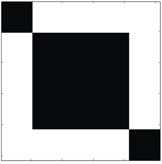
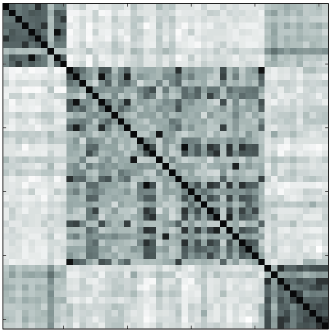
(c) 16S	(d) gyrB (20% missing)
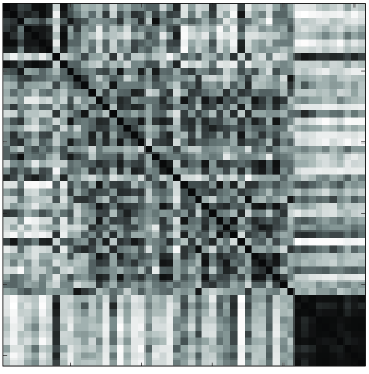
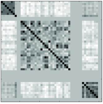
(e) completed matrix	(f) estimated matrix

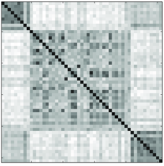
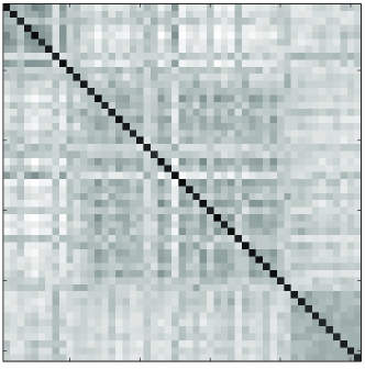
Figure 2: An example of kernel matrix completion. See the text for details.

Figure 3: Clustering performance of the completed matrix. The solid curve shows the averaged ARI of the completed matrix, and the error bar describes the standard deviation. The upper and lower flat lines show the ARIs of the complete gyrB and 16S kernel matrices, respectively.

Figure 4: Clustering performance of the estimated matrix. The solid curve shows the averaged ARI of the estimated matrix, and the error bar describes the standard deviation.

7 Possible Extension

As we related the em algorithm to maximum likelihood inference in Sec. 5, it is straightforward to generalize it to the maximum a posteriori (MAP) inference or more generally the Bayes inference (Robert, 1994). For example, we are going to modify the em algorithm to obtain the MAP estimate. The MAP estimation amounts to minimizing the KL divergence penalized by a prior,

$$KL(D,M)-\log\pi(M),\qquad D\in{\cal D},\quad M\in{\cal M},$$

where $\pi(M)$ is a prior distribution for $M$. Since the additional term $-\log\pi(M)$ depends only on the model $M$, only the $m$-step is changed so as to minimize the above objective function with respect to $M$.

Let us give a simple example of MAP estimation in the spectral variants case. In Bayesian inference, it is common to take a conjugate prior, so that the posterior distribution remains as a member of the exponential family. Since the model parameter ${\boldsymbol{b}}$ is related to a covariance matrix, we choose the Gamma distribution, which works as a conjugate prior for the variance of Gaussian distribution (Robert, 1994). The prior distribution is defined independently for each $b_{j}$ as

$$\pi(b_{j};\,\nu,\alpha)=\frac{1}{\Gamma(\nu)\alpha^{\nu}}\exp\left\{-\frac{b_{j}}{\alpha}+(\nu-1)\log b_{j}\right\},$$

where $\nu$ and $\alpha$ denote hyperparameters, by which the mean and the variance are specified by $E(b_{j})=\alpha\nu$ and $V(b_{j})=\alpha^{2}\nu$. The $m$ step for MAP estimation is to minimize

$$L_{m}^{\rm MAP}=L_{m}-\sum_{j=1}^{\ell}\log\pi(b_{j};\,\nu,\alpha),$$

which leads to the equation

$$\operatorname{tr}(M_{i}(\sum_{j=1}^{c}b_{j}M_{j})^{-1})+\frac{\nu-1}{b_{i}}=\operatorname{tr}(M_{i}D)+\frac{1}{\alpha},\qquad i=1,\ldots,\ell.$$

In the spectral variants case, the left hand side is reduced to $\nu/b_{i}$, thus we obtain the MAP solution in a closed form as

$$b_{i}=\frac{\nu}{\operatorname{tr}(M_{i}D)+1/\alpha},\qquad i=1,\ldots,\ell.$$

8 Conclusion

In this paper, we introduced the information geometry in the space of kernel matrices, and applied the em algorithm in matrix approximation. The main difference to other Euclidean methods is that we use the KL divergence. In general, we cannot determine which distance is better, because it is highly data dependent. However our method has a great utility, because it can be implemented only with algebraic computation and we do not need any specialized optimizer such as semidefinite programmming unlike (Graepel, 2002; Cristianini et al., 2002; Lanckriet et al., 2002).

One of our contribution is that we related matrix approximation to statistical inference in Sec. 5. Thus, in future works, it would be interesting to involve advanced methods in statistical inference, such as generalized EM (Dempster et al., 1977) and variational Bayes (Attias, 1999). Also we are looking forward to apply our method to diverse kinds of real data which are not limited to bioinformatics.

Appendix A Analytical Solvability of the $m$-step

In this appendix, we discuss the solvability of the $m$-step. The left hand side of (14) is the $m$-coordinate of the submanifold $\cal M$, while $b_{j}$ denote the $e$-coordinate of $\cal M$. The $e$-coordinate and $m$-coordinate are connected by the Legendre transform (Amari and Nagaoka, 2001). In the mother manifold ${\cal P}$, the Legendre transform is easily obtained as the inverse of the matrix. In the submanifold $\cal M$ of $\cal P$, however, it is difficult to obtain the Legendre transform in general. The difficulty is caused by the difference of geodesics defined in $\cal M$ and $\cal P$. When the geodesic defined by a coordinate system of a submanifold ${\cal S}\subseteq{\cal P}$ coincides the geodesic defined by the corresponding global coordinate system of ${\cal P}$, the submanifold is called autoparallel. In our case, $\cal M$ is autoparallel for the $e$-coordinate, but it is not always autoparallel for the $m$-coordinate. When the submanifold is autoparallel for the both coordinate systems, the submanifold is called doubly autoparallel.

Let us consider when a submanifold becomes doubly autoparallel. To begin with, let us define the product $*$ between two $d\times d$ symmetric matrices $X,Y\in{\it Sym}(d)$,

$$X*Y=\frac{1}{2}(XY+YX).$$ (16)

The algebra equipped with the usual matrix sum and the product (16) is called the Jordan algebra of the vector space of Sym$(d)$. The following theorem provides the necessary and sufficient condition for doubly autoparallel submanifold.

Theorem 1 (Ohara (1999), Theorem 4.6).

Assume the identity matrix $I$ is an element of the submanifold $\cal M$, Then $\cal M$ is doubly autoparallel if and only if the tangent space of $\cal M$ is a Jordan subalgebra of Sym$(d)$.

When a submanifold ${\cal M}\subseteq{\cal P}$ is determined as (15), ${\cal M}$ is doubly autoparallel if the following holds for all $i,j$:

$$N_{i}*N_{j}\in\mathrm{span}(\{N_{1},\ldots,N_{c}\}).$$

Ohara (1999) has shown that, if and only if ${\cal M}$ is doubly autoparallel, the $m$-projection can be solved analytically, that is, the optimal solution is obtained by one Newton step. For example, in the spectral variants case, $N_{i}={\boldsymbol{v}}_{i}{\boldsymbol{v}}_{i}^{\top}$ and

$$N_{i}*N_{j}=0\in\mathrm{span}(\{N_{1},\ldots,N_{c}\}).$$

Thus the $m$-projection is obtained analytically in this case.

References

- Amari (1995) S. Amari. Information geometry of the EM and em algorithms for neural networks. Neural Networks, 8(9):1379–1408, 1995.
- Amari and Nagaoka (2001) S. Amari and H. Nagaoka. Methods of Information Geometry, volume 191 of Translations of Mathematical Monographs. American Mathematical Society, 2001.
- Attias (1999) H. Attias. Inferring parameters and structure of latent variable models by variational Bayes. In Uncertainty in Artificial Intelligence: Proceedings of the Fifteenth Conference (UAI-1999), pages 21–30, San Francisco, CA, 1999. Morgan Kaufmann Publishers.
- Brown (1999) T.A. Brown. Genomes. BIOS Scientific Publishers, 1999.
- Cristianini et al. (2002) N. Cristianini, J. Shawe-Taylor, J. Kandola, and A. Elisseeff. On kernel-target alignment. In T.G. Dietterich, S. Becker, and Z. Ghahramani, editors, Advances in Neural Information Processing Systems 14. MIT Press, 2002.
- Dempster et al. (1977) A.P. Dempster, N.M. Laird, and D.B. Rubin. Maximum likelihood from incomplete data via the em algorithm. J. Roy. Stat. Soc. B, 39:1–38, 1977.
- Graepel (2002) T. Graepel. Kernel matrix completion by semidefinite programming. In Proc. ICANN’02, pages 687–693, 2002.
- Hubert and Arabie (1985) L. Hubert and P. Arabie. Comparing partitions. J. Classif., pages 193–218, 1985.
- Ikeda et al. (1999) S. Ikeda, S. Amari, and H. Nakahara. Convergence of the wake-sleep algorithm. In M.S. Kearns, S.A. Solla, and D.A. Cohn, editors, Advances in Neural Information Processing Systems 11, pages 239–245. MIT Press, 1999.
- Kasai et al. (1998) H. Kasai, A. Bairoch, K. Watanabe, K. Isono, S. Harayama, E. Gasteiger, and S. Yamamoto. Construction of the gyrB database for the identification and classification of bacteria. In Genome Informatics 1998, pages 13–21. Universal Academic Press, 1998.
- Lanckriet et al. (2002) G. Lanckriet, N. Cristianini, P. Bartlett, L. El Ghaoui, and M.I. Jordan. Learning the kernel matrix with semi-definite programming. In Proc. ICML’02, 2002.
- Ohara (1999) A. Ohara. Information geometric analysis of an interior point method for semidefinite programming. In O.E. Barndorff-Nielsen and E.B. Vedel Jensen, editors, Geometry in Present Day Science, pages 49–74. World Scientific, 1999.
- Ohara et al. (1996) A. Ohara, N. Suda, and S. Amari. Dualistic differential geometry of positive definite matrices and its applications to related problems. Linear Algebra and Its Applications, 247:31–53, 1996.
- Robert (1994) C.P. Robert. The Bayesian Choice: A Decision-Theoretic Motivation. Springer Verlag, 1994.
- Schölkopf and Smola (2001) B. Schölkopf and A. J. Smola. Learning with Kernels. MIT Press, Cambridge, MA, 2001.
- Tsuda et al. (2002) K. Tsuda, T. Kin, and K. Asai. Marginalized kernels for biological sequences. Bioinformatics, 18(Suppl. 1):S268–S275, 2002.
- Vapnik (1998) V.N. Vapnik. Statistical Learning Theory. Wiley, New York, 1998.
- Vert and Kanehisa (2002) J.-P. Vert and M. Kanehisa. Graph-driven features extraction from microarray data. Technical Report physics/0206055, Arxiv, June 2002.
- Yamamoto et al. (2000) S. Yamamoto, H. Kasai, D.L. Arnold, R.W. Jackson, A. Vivian, and S. Harayama. Phylogeny of the genus Pseudomonas: intrageneric structure reconstructed from the nucleotide sequences of gyrB and rpoD genes. Microbiology, 146:2385–2394, 2000.
- Yeung and Ruzzo (2001) K.Y. Yeung and W.L. Ruzzo. Principal component analysis for clustering gene expression data. Bioinformatics, 17(9):763–774, 2001.