Maximing the Margin in the Input Space

Abstract

We propose a novel criterion for support vector machine learning: maximizing the margin in the input space, not in the feature (Hilbert) space. This criterion is a discriminative version of the principal curve proposed by Hastie et al. The criterion is appropriate in particular when the input space is already a well-designed feature space with rather small dimensionality. The definition of the margin is generalized in order to represent prior knowledge. The derived algorithm consists of two alternating steps to estimate the dual parameters. Firstly, the parameters are initialized by the original SVM. Then one set of parameters is updated by Newton-like procedure, and the other set is updated by solving a quadratic programming problem. The algorithm converges in a few steps to a local optimum under mild conditions and it preserves the sparsity of support vectors. Although the complexity to calculate temporal variables increases the complexity to solve the quadratic programming problem for each step does not change. It is also shown that the original SVM can be seen as a special case. We further derive a simplified algorithm which enables us to use the existing code for the original SVM.

1 Introduction

The support vector machine (SVM) is known as one of state-of-the-art methods especially for pattern recognition [3, 7, 12]. The original SVM maximizes the margin which is defined by the minimum distance between samples and a separating hyperplane in a Hilbert space $\mathcal{H}$. Even when the dimensionality of $\mathcal{H}$ is very large, it has been proved that the original SVM has a bound for a generalization error which is independent of the dimensionality. In practice, however, the original SVM sometimes gives a very small margin in the input space, because the metric of the feature space is usually quite different from that of the input space. Such a situation is undesirable in particular when the input space is already a well-designed feature space by using some prior knowledge[2, 4, 6, 10, 11].

This paper gives a learning algorithm to maximize the margin in the input space. One difficulty is getting an explicit form of the margin in the input space, because the classification boundary is curved and the vertical projection from a sample point to the boundary is not always unique. We solve this problem by linear approximation techniques. The derived algorithm basically consists of iterations of the alternating two stages as follows: one is to estimate the projection point and the other is to solve a quadratic programming to find optimal parameter values.

Such a dual structure appears in other frameworks, such as EM algorithm and variational Bayes. Much more related work is the principal curve proposed by Hastie et al[5]. The principal curve finds a curve in a ‘center’ of the points in the input space.

The derived algorithm is not a gradient-descent type but Newton-like; hence we have to investigate its convergence property. It is shown that the derived algorithm does not always converges to the global optimum, but it converges to a local optimum under mild conditions. Some interesting relations to the original SVM are also shown: the original SVM can be seen as a special case of the algorithm; and the number of support vectors does not increase so much from the original SVM. The algorithm is verified through simple simulations.

2 Generalized margin in the input space

We consider a binary classification problem. The purpose of learning is to construct a map from an $m$-dimensional input $\mbox{\boldmath$x$}\in{\Re}^{m}$ to a corresponding output $y\in\{\pm 1\}$ by using a finite number of samples $(\mbox{\boldmath$x$}_{1},y_{1}),\ldots,(\mbox{\boldmath$x$}_{n},y_{n})$.

Let us consider a linear classifier, $y=\mbox{sgn}[f(\mbox{\boldmath$x$})]$, where $f(\mbox{\boldmath$x$})\equiv\omega\cdot\phi(\mbox{\boldmath$x$})+f_{0}$; $\phi(\mbox{\boldmath$x$})$ is a feature of an input $x$ in a Hilbert space $\mathcal{H}$, $\omega\in\mathcal{H}$ is a weight parameter and $f_{0}\in\Re$ is a bias parameter. Those parameters $\omega$ and $f_{0}$ define a separating hyperplane in the feature space. As a feature function $\phi(\mbox{\boldmath$x$})$, we only consider a differentiable nonlinear map.

A margin in the input space is defined by the minimum distance from sample points to the classification boundary in the input space. Since the classification boundary forms a complex curved surface, the distance cannot be obtained in an explicit form, and more significantly, a projection from a point to the boundary is not unique.

Here, the metric in the input space is not necessary to be Euclidean. Some Riemannian metric $G(\mbox{\boldmath$x$})$ may be defined, which enables us to represent many kinds of prior knowledge. For example, the invariance of patterns[7, 10] can be implemented in this form. Another example is that Fisher information matrix is a natural metric, when the input space is a parameter space of some probability distribution[2, 6]. Although the distance is theoretically preferable to be measured by the length of a geodesic in the Riemannian space, it causes computational difficulty. In our formulation, since we only need a distance from a sample point to another point, we use a computationally feasible (nonsymmetric) distance from a sample point $\mbox{\boldmath$x$}_{i}$ to another point $x$ in the quadratic norm,

$$\|\mbox{\boldmath$x$}-\mbox{\boldmath$x$}_{i}\|_{G_{i}}^{2}=(\mbox{\boldmath$x$}-\mbox{\boldmath$x$}_{i})^{\mathsf{T}}G_{i}(\mbox{\boldmath$x$}-\mbox{\boldmath$x$}_{i}),$$

where $G_{i}\equiv G(\mbox{\boldmath$x$}_{i})$.

For simplicity, we mainly consider the hard margin case in which sample points are separable by a hyperplane in the Hilbert space. The soft margin case is discussed in the section 5.

Let ${\mbox{\boldmath$x$}}^{*}_{i}$ be the closest point on the boundary surface from a sample point $\mbox{\boldmath$x$}_{i}$, and $\mbox{\boldmath$d$}_{i}\equiv{\mbox{\boldmath$x$}}^{*}_{i}-\mbox{\boldmath$x$}_{i}$. Since $\mbox{\boldmath$d$}_{i}$ is invariant under a scalar transformation of $(\omega,f_{0})$, we can assume all points are separated with satisfying

$$\|\mbox{\boldmath$d$}_{i}\|_{G_{i}}^{2}\geq{1/\omega\cdot\omega},\quad i=1,\cdots,n,$$ (1)

If we assume at least one of them is an equality, the margin is given by $1/\sqrt{\omega\cdot\omega}$. Then we can find the optimal parameter by minimizing a quadratic objective function $\omega\cdot\omega$ with the constraints (1) and $y_{i}f(\mbox{\boldmath$x$}_{i})>0$.

In order to solve the optimization problem, we start from a solution of the original SVM and update the solution iteratively. By two kinds of linearization technique and a kernel trick which are described in the next section, we obtain a discriminant function at the $k$-th iteration step in the form of

$$f(\mbox{\boldmath$x$})=\sum_{i\in\mathrm{S.V.}}\{a_{i}^{(k)}\mathrm{k}(\hat{\mbox{\boldmath$x$}}_{i}^{(k)},\mbox{\boldmath$x$})+\mbox{\boldmath$b$}_{i}^{(k)}{}^{\mathsf{T}}\mathbf{k}_{x}(\hat{\mbox{\boldmath$x$}}_{i}^{(k)},\mbox{\boldmath$x$})\}+f_{0}^{(k)},$$ (2)

where S.V. is a set of indices of support vectors, $\mathrm{k}(\mbox{\boldmath$x$},\mbox{\boldmath$y$})$ is a kernel function and $\mathbf{k}_{x}(\mbox{\boldmath$x$},\mbox{\boldmath$y$})$ is its derivative defined by $\mathbf{k}_{x}(\mbox{\boldmath$x$},\mbox{\boldmath$y$})\equiv{\partial\mathrm{k}(\mbox{\boldmath$x$},\mbox{\boldmath$y$})/\partial\mbox{\boldmath$x$}}$. We have two groups of parameters here: One is of $a_{i}$, $\mbox{\boldmath$b$}_{i}$ and $f_{0}$ which are parameters of linear coefficients, and the other is of $\hat{\mbox{\boldmath$x$}}_{i}$ which is an estimate of the projection point ${\mbox{\boldmath$x$}}^{*}_{i}$ and forms base functions. $a_{i}$ and $f_{0}$ are initialized by the corresponding parameters in the original SVM and the other parameters are initialized by $\mbox{\boldmath$b$}_{i}=\mathbf{0}$, $\hat{\mbox{\boldmath$x$}}_{i}=\mbox{\boldmath$x$}_{i}$.

3 Iterative QP by linear approximations

In this section, we overview the derivation of update rules of those parameters. The resultant algorithm is summarized in sec.3.6.

3.1 Linear approximation of the distance to the boundary

Suppose an estimated projection point $\hat{\mbox{\boldmath$x$}}_{i}$ is given, we can get an approximate distance $\|\mbox{\boldmath$d$}_{i}\|_{G_{i}}$ by a linear approximation[1]. Taking the Taylor expansion of
$f({\mbox{\boldmath$x$}}^{*}_{i})=0$ around $\hat{\mbox{\boldmath$x$}}_{i}$ up to the first order, we obtain a constraint on $\mbox{\boldmath$d$}_{i}$,

$$f(\hat{\mbox{\boldmath$x$}}_{i})+\nabla f(\hat{\mbox{\boldmath$x$}}_{i})^{\mathsf{T}}(\mbox{\boldmath$d$}_{i}-\hat{\mbox{\boldmath$d$}}_{i})=0,$$

where $\hat{\mbox{\boldmath$d$}}_{i}=\hat{\mbox{\boldmath$x$}}_{i}-\mbox{\boldmath$x$}_{i}$. Minimizing $\|\mbox{\boldmath$d$}_{i}\|_{G_{i}}^{2}$ under this constraint, we have

$$\|\mbox{\boldmath$d$}_{i}\|_{G_{i}}^{2}={(\omega\cdot\{\phi(\hat{\mbox{\boldmath$x$}}_{i})-\mbox{\boldmath$\psi$}(\hat{\mbox{\boldmath$x$}}_{i})^{\mathsf{T}}\hat{\mbox{\boldmath$d$}}_{i}\}+f_{0})^{2}\over\|\omega\cdot\mbox{\boldmath$\psi$}(\hat{\mbox{\boldmath$x$}}_{i})\|_{G_{i}^{-1}}^{2}},$$ (3)

where $\mbox{\boldmath$\psi$}(\hat{\mbox{\boldmath$x$}}_{i})\equiv\nabla\phi(\hat{\mbox{\boldmath$x$}}_{i})\in{\mathcal{H}}^{m}$. Note that this approximate value is unique, and it is invariant under a scalar transformation of $(\omega,f_{0})$. Moreover, the approximation is strictly correct when $\hat{\mbox{\boldmath$x$}}_{i}={\mbox{\boldmath$x$}}^{*}_{i}$ and $\nabla f({\mbox{\boldmath$x$}}^{*}_{i})\neq 0$.

3.2 Linearization of the constraint

Using the approximate value of the distance, we have a nonlinear constraint,

$$y_{i}\left[\omega\cdot\{\phi(\hat{\mbox{\boldmath$x$}}_{i})-\mbox{\boldmath$\psi$}(\hat{\mbox{\boldmath$x$}}_{i})^{\mathsf{T}}\hat{\mbox{\boldmath$d$}}_{i}\}+f_{0}\right]\geq{\|\omega\cdot\mbox{\boldmath$\psi$}(\hat{\mbox{\boldmath$x$}}_{i})\|_{G_{i}^{-1}}\over\sqrt{\omega\cdot\omega}}.$$ (4)

Since the constraint is nonlinear for $\omega$, we linearize it around an approximate solution $\omega=\hat{\omega}$ which is the solution at a current step. This linearization not only simplifies the problem, but also enables us to derive a dual problem.

Let $g_{i}(\omega)$ be the right hand side of (4), the first order expansion is

$$g_{i}(\omega)=g_{i}(\hat{\omega})+\left({\partial g_{i}(\hat{\omega})/\partial\omega}\right)\cdot(\omega-\hat{\omega}).$$

Now let $\hat{g}_{i}\equiv g_{i}(\hat{\omega}),\hat{\eta}_{i}\equiv{\partial g_{i}(\hat{\omega})/\partial\omega}$, then we have a linear constraint for $\omega$,

$$\omega\cdot[y_{i}\ \{\phi(\hat{\mbox{\boldmath$x$}}_{i})-\mbox{\boldmath$\psi$}(\hat{\mbox{\boldmath$x$}}_{i})^{\mathsf{T}}\hat{\mbox{\boldmath$d$}}_{i}\}-\hat{\eta}_{i}]\geq\hat{g}_{i}-f_{0}y_{i},$$ (5)

where we used the fact $\hat{\omega}\cdot\hat{\eta}_{i}=0$. Suppose $\hat{\mbox{\boldmath$q$}}_{i}\equiv\hat{\omega}\cdot\mbox{\boldmath$\psi$}(\hat{\mbox{\boldmath$x$}}_{i})$ and $\hat{r}\equiv\hat{\omega}\cdot\hat{\omega}$, then $\hat{g}_{i}$ and $\hat{\eta}_{i}$ are given by

$$\hat{g}_{i} = {1\over\sqrt{\hat{r}}}\|\hat{\mbox{\boldmath$q$}}_{i}\|_{G_{i}^{-1}},$$

$$\hat{\eta}_{i} = {1\over\hat{g}_{i}\hat{r}}\left\{\hat{\mbox{\boldmath$q$}}_{i}^{\mathsf{T}}G_{i}^{-1}\mbox{\boldmath$\psi$}(\hat{\mbox{\boldmath$x$}}_{i})-{1\over\hat{r}}\|\hat{\mbox{\boldmath$q$}}_{i}\|_{G_{i}^{-1}}^{2}\hat{\omega}\right\}.$$ (6)

By the above linearization, we can derive the dual problem in a similar way to the original SVM,

$$W(\mbox{\boldmath$\alpha$})=\sum_{i}\hat{g}_{i}\alpha_{i}$$

$$-{1\over 2}\sum_{i,j}\alpha_{i}\alpha_{j}[y_{i}\{\phi(\hat{\mbox{\boldmath$x$}}_{i})-\mbox{\boldmath$\psi$}(\hat{\mbox{\boldmath$x$}}_{i})^{\mathsf{T}}\hat{\mbox{\boldmath$d$}}_{i}\}-\hat{\eta}_{i}]\cdot[y_{j}\{\phi(\hat{\mbox{\boldmath$x$}}_{j})-\mbox{\boldmath$\psi$}(\hat{\mbox{\boldmath$x$}}_{j})^{\mathsf{T}}\hat{\mbox{\boldmath$d$}}_{j}\}-\hat{\eta}_{j}],$$

which is maximized under constraints $\alpha_{i}\geq 0$
and $\sum_{i}\alpha_{i}y_{i}=0$. The solution $\omega$ is given by

$$\omega=\sum_{i}\alpha_{i}[y_{i}\{\phi(\hat{\mbox{\boldmath$x$}}_{i})-\mbox{\boldmath$\psi$}(\hat{\mbox{\boldmath$x$}}_{i})^{\mathsf{T}}\hat{\mbox{\boldmath$d$}}_{i}\}-\hat{\eta}_{i}].$$ (7)

Here we can see an apparent relation to the original SVM, i.e., by letting $\hat{\mbox{\boldmath$x$}}_{i}=\mbox{\boldmath$x$}_{i}$, $\hat{\eta}_{i}=0$, and $\hat{g}_{i}=1$, we have the exactly the same optimization problem as the original SVM.

3.3 Kernel trick

In order to avoid the calculation of mapping into high dimensional Hilbert space, SVM applies a kernel trick, by which an inner product is replaced by a symmetric positive definite kernel function (Mercer kernel) that is easy to calculate[9, 3, 7, 12]. In our formulation, $\phi(\mbox{\boldmath$x$})\cdot\phi(\mbox{\boldmath$y$})$ is replaced by a Mercer kernel $\mathrm{k}(\mbox{\boldmath$x$},\mbox{\boldmath$y$})$. We also have to calculate the inner product related to $\psi$ (the derivative of $\phi$). Let us assume that the kernel function $\mathrm{k}$ is differentiable. Then, $\mbox{\boldmath$\psi$}(\mbox{\boldmath$x$})\cdot\phi(\mbox{\boldmath$y$})$ is replaced by a vector $\mathbf{k}_{x}(\mbox{\boldmath$x$},\mbox{\boldmath$y$})\equiv{\partial\mathrm{k}(\mbox{\boldmath$x$},\mbox{\boldmath$y$})/\partial\mbox{\boldmath$x$}}$, and $\mbox{\boldmath$\psi$}(\mbox{\boldmath$x$})\cdot\mbox{\boldmath$\psi$}(\mbox{\boldmath$y$})^{\mathsf{T}}$ is replaced by a matrix $\mathrm{K}_{xy}(\mbox{\boldmath$x$},\mbox{\boldmath$y$})\equiv{\partial^{2}\mathrm{k}(\mbox{\boldmath$x$},\mbox{\boldmath$y$})/\partial\mbox{\boldmath$x$}\partial\mbox{\boldmath$y$}^{\mathsf{T}}}$.

Now we can derive the kernel version of the optimization problem. In (7), $\hat{\eta}_{i}\in\mathcal{H}$ has bases related to $\mbox{\boldmath$\psi$}(\hat{\mbox{\boldmath$x$}}_{i})$ and $\hat{\omega}$, and the solution $\omega$ has bases $\phi(\hat{\mbox{\boldmath$x$}}_{i})$ additionally. Although $\hat{\omega}$ can have any kinds of bases, we restrict it in the following form to avoid increasing number of bases.

$$\hat{\omega}=\sum_{i}\{\hat{a}_{i}\phi(\hat{\mbox{\boldmath$x$}}_{i})+\hat{\mbox{\boldmath$b$}}_{i}^{\mathsf{T}}\mbox{\boldmath$\psi$}(\hat{\mbox{\boldmath$x$}}_{i})\}.$$

Then we have $\hat{\mbox{\boldmath$q$}}_{i}=\sum_{j}\{\hat{a}_{j}\mathbf{k}_{x}(\hat{\mbox{\boldmath$x$}}_{i},\hat{\mbox{\boldmath$x$}}_{j})+\mathrm{K}_{xy}(\hat{\mbox{\boldmath$x$}}_{i},\hat{\mbox{\boldmath$x$}}_{j})\hat{\mbox{\boldmath$b$}}_{j}\}$. Now let

$$\hat{p}_{i}\equiv\hat{\omega}\cdot\phi(\hat{\mbox{\boldmath$x$}}_{i})=\sum_{j}\{\hat{a}_{j}\mathrm{k}(\hat{\mbox{\boldmath$x$}}_{j},\hat{\mbox{\boldmath$x$}}_{i})+\hat{\mbox{\boldmath$b$}}_{j}^{\mathsf{T}}\mathbf{k}_{x}(\hat{\mbox{\boldmath$x$}}_{j},\hat{\mbox{\boldmath$x$}}_{i})\},$$

then $\hat{r}$ is given by $\hat{r}=\sum_{i}(\hat{a}_{i}\hat{p}_{i}+\hat{\mbox{\boldmath$b$}}_{i}^{\mathsf{T}}\hat{\mbox{\boldmath$q$}}_{i})$, and $\hat{g}_{i}$ by (3.2). Further, let us define additional temporal variables that represent several terms in the objective function,

$$\hat{s}_{ij} \equiv \{\phi(\hat{\mbox{\boldmath$x$}}_{i})-\mbox{\boldmath$\psi$}(\hat{\mbox{\boldmath$x$}}_{i})^{\mathsf{T}}\hat{\mbox{\boldmath$d$}}_{i}\}\cdot\{\phi(\hat{\mbox{\boldmath$x$}}_{j})-\mbox{\boldmath$\psi$}(\hat{\mbox{\boldmath$x$}}_{j})^{\mathsf{T}}\hat{\mbox{\boldmath$d$}}_{j}\}$$

$$= \mathrm{k}(\hat{\mbox{\boldmath$x$}}_{i},\hat{\mbox{\boldmath$x$}}_{j})+\hat{\mbox{\boldmath$d$}}_{i}^{\mathsf{T}}\mathrm{K}_{xy}(\hat{\mbox{\boldmath$x$}}_{i},\hat{\mbox{\boldmath$x$}}_{j})\hat{\mbox{\boldmath$d$}}_{j}-\hat{\mbox{\boldmath$d$}}_{i}^{\mathsf{T}}\mathbf{k}_{x}(\hat{\mbox{\boldmath$x$}}_{i},\hat{\mbox{\boldmath$x$}}_{j})-\hat{\mbox{\boldmath$d$}}_{j}^{\mathsf{T}}\mathbf{k}_{x}(\hat{\mbox{\boldmath$x$}}_{j},\hat{\mbox{\boldmath$x$}}_{i}),$$

$$\hat{t}_{ij} \equiv \hat{\eta}_{i}\cdot\{\phi(\hat{\mbox{\boldmath$x$}}_{j})-\mbox{\boldmath$\psi$}(\hat{\mbox{\boldmath$x$}}_{j})^{\mathsf{T}}\hat{\mbox{\boldmath$d$}}_{j}\}$$

$$= {1\over\hat{g}_{i}\hat{r}}\bigg{\{}\hat{\mbox{\boldmath$q$}}_{i}^{\mathsf{T}}G_{i}^{-1}\left(\mathbf{k}_{x}(\hat{\mbox{\boldmath$x$}}_{i},\hat{\mbox{\boldmath$x$}}_{j})-\mathrm{K}_{xy}(\hat{\mbox{\boldmath$x$}}_{i},\hat{\mbox{\boldmath$x$}}_{j})\hat{\mbox{\boldmath$d$}}_{j}\right)-{\|\hat{\mbox{\boldmath$q$}}_{i}\|_{G_{i}^{-1}}^{2}\over\hat{r}}(\hat{p}_{j}-\hat{\mbox{\boldmath$d$}}_{j}^{\mathsf{T}}\hat{\mbox{\boldmath$q$}}_{j})\bigg{\}},$$

$$\hat{u}_{ij} = \hat{\eta}_{i}\cdot\hat{\eta}_{j}={1\over\hat{g}_{i}\hat{g}_{j}\hat{r}^{2}}(\hat{\mbox{\boldmath$q$}}_{i}^{\mathsf{T}}G_{i}^{-1}\mathrm{K}_{xy}(\hat{\mbox{\boldmath$x$}}_{i},\hat{\mbox{\boldmath$x$}}_{j})G_{j}^{-1}\hat{\mbox{\boldmath$q$}}_{j}-{\|\hat{\mbox{\boldmath$q$}}_{i}\|_{G_{i}^{-1}}^{2}\|\hat{\mbox{\boldmath$q$}}_{j}\|_{G_{j}^{-1}}^{2}\over\hat{r}}),$$

then we have the objective function in a kernel form,

$$W(\mbox{\boldmath$\alpha$})=\sum_{i}\hat{g}_{i}\alpha_{i}-{1\over 2}\sum_{i,j}\alpha_{i}\alpha_{j}(y_{i}y_{j}\hat{s}_{ij}-y_{j}\hat{t}_{ij}-y_{i}\hat{t}_{ji}+\hat{u}_{ij}),$$ (8)

which is maximized under constraints

$$\alpha_{i}\geq 0,\qquad\sum_{i}y_{i}\alpha_{i}=0.$$ (9)

The new parameters can be determined from (7) by

$$a_{i}^{(k+1)} = \alpha_{i}y_{i}+\beta\hat{a}_{i},$$

$$\mbox{\boldmath$b$}_{i}^{(k+1)} = -\alpha_{i}\left(y_{i}\hat{\mbox{\boldmath$d$}}_{i}+{G_{i}^{-1}\hat{\mbox{\boldmath$q$}}_{i}\over\hat{g}_{i}\hat{r}}\right)+\beta\hat{\mbox{\boldmath$b$}}_{i},$$ (10)

where $\beta=\sum_{j}{\alpha_{j}\|\hat{\mbox{\boldmath$q$}}_{j}\|_{G_{i}^{-1}}^{2}/\hat{g}_{j}\hat{r}^{2}}$.

As for the bias term $f_{0}$, since the constraint (5) should be satisfied in equality for $J=\{i\mid\alpha_{i}\neq 0\}$ from the Kuhn-Tucker condition, we have for any $i\in J$,

$$f_{0}^{(k+1)}=y_{i}\hat{g}_{i}-\sum_{j}\alpha_{j}(y_{j}\hat{s}_{ji}-\hat{t}_{ji}-y_{i}y_{j}\hat{t}_{ij}+y_{i}\hat{u}_{ij})$$ (11)

From (3.3), we can estimate the number of support vectors. Let $J_{k}$ be the indices of nonzero $\alpha_{i}$’s at the $k$-th step, then the number of support vectors is bounded from upper by $|J_{0}\cup J_{1}\cup\cdots\cup J_{k}|$. Since $J_{k}$ does not change much as long as the structure of classification boundary is similar, the number of support vectors is expected to be not so larger than the original SVM.

3.4 Update of the approximate projection of the points

To complete the algorithm, we have to consider the update of the approximate value of the projection point $\hat{\mbox{\boldmath$x$}}_{i}$ which is initialized by $\mbox{\boldmath$x$}_{i}$, otherwise the convergent solution is not precise what we want. If good approximates $\hat{\omega}$ and $\hat{f}_{0}$ of the solution are given, we can refine $\hat{\mbox{\boldmath$x$}}_{i}$ iteratively in the same way as in sec. 3.1: Suppose $\hat{\omega}=\sum_{j}\{\hat{a}_{j}\phi(\hat{\mbox{\boldmath$x$}}_{j}^{\mathrm{old}})+\hat{\mbox{\boldmath$b$}}_{j}^{\mathsf{T}}\mbox{\boldmath$\psi$}(\hat{\mbox{\boldmath$x$}}_{j}^{\mathrm{old}})\}$, the projection point $\hat{\mbox{\boldmath$x$}}_{i}$ can be estimated by iterating the following steps for $l=0,1,2,3,\cdots$,

$$\hat{\mbox{\boldmath$x$}}_{i}^{[l+1]}=\mbox{\boldmath$x$}_{i}-{\hat{\mbox{\boldmath$q$}}_{i}^{[l]}\over\|\hat{\mbox{\boldmath$q$}}_{i}^{[l]}\|_{G_{i}^{-1}}^{2}}\left[\hat{p}_{i}^{[l]}-(\hat{\mbox{\boldmath$x$}}_{i}^{[l]}{}-\mbox{\boldmath$x$}_{i})^{\mathsf{T}}\hat{\mbox{\boldmath$q$}}_{i}^{[l]}+\hat{f}_{0}\right]$$ (12)

where $\hat{\mbox{\boldmath$x$}}_{i}^{[0]}$ is initialized by $\hat{\mbox{\boldmath$x$}}_{i}^{\mathrm{old}}$; $\hat{p}_{i}^{[l]}$ and $\hat{\mbox{\boldmath$q$}}_{i}^{[l]}$ are defined in a similar way as $\hat{p}_{i}$ and $\hat{\mbox{\boldmath$q$}}_{i}$,

$$\hat{p}_{i}^{[l]} \equiv \hat{\omega}\cdot\phi(\hat{\mbox{\boldmath$x$}}_{i}^{[l]})$$

$$= \sum_{j}\{\hat{a}_{j}\mathrm{k}(\hat{\mbox{\boldmath$x$}}_{j}^{\mathrm{old}},\hat{\mbox{\boldmath$x$}}_{i}^{[l]})+\hat{\mbox{\boldmath$b$}}_{j}^{\mathsf{T}}\mathbf{k}_{x}(\hat{\mbox{\boldmath$x$}}_{j}^{\mathrm{old}},\hat{\mbox{\boldmath$x$}}_{i}^{[l]})\},$$

$$\hat{\mbox{\boldmath$q$}}_{i}^{[l]} \equiv \hat{\omega}\cdot\mbox{\boldmath$\psi$}(\hat{\mbox{\boldmath$x$}}_{i}^{[l]})$$

$$= \sum_{j}\{\hat{a}_{j}\mathbf{k}_{x}(\hat{\mbox{\boldmath$x$}}_{i}^{[l]},\hat{\mbox{\boldmath$x$}}_{j}^{\mathrm{old}})+\mathrm{K}_{xy}(\hat{\mbox{\boldmath$x$}}_{i}^{[l]},\hat{\mbox{\boldmath$x$}}_{j}^{\mathrm{old}})\hat{\mbox{\boldmath$b$}}_{j}\}.$$

Note that locally maximum points and saddle points of the distance are also equilibrium states of (12). The following proposition guarantees such a point is not stable.

Proposition 1

A point $\hat{\mbox{\boldmath$x$}}_{i}\in{\Re}^{m}$ is an equilibrium state of the iteration step (12), when and only when the point is a critical point of the distance from $\mbox{\boldmath$x$}_{i}$ to the separating boundary, i.e., a local minimum, a local maximum or a saddle point. The equilibrium state is not stable when the point is a local maximum or a saddle point.

Proof: It is straightforward to show that a point is an equillibrium state of the iteration step (12), only when the point is a critical point of the projection point $\|\mbox{\boldmath$d$}_{i}\|_{G_{i}}^{2}$. Without loss of generality, we can assume the uniform metric case $G_{i}=I$, because update rule (12) is invariant of a metric transformation. We consider the behavior around a critical point ${\mbox{\boldmath$x$}}^{*}_{i}$. Let $\hat{\mbox{\boldmath$x$}}_{i}^{[l]}={\mbox{\boldmath$x$}}^{*}_{i}+\mbox{\boldmath$\varepsilon$}$, for a sufficiently small vector $\varepsilon$. One can show that $\hat{\mbox{\boldmath$x$}}_{i}^{[l]}$ is mapped into the separating hypersurface $f(\mbox{\boldmath$x$})=\hat{\omega}\cdot\phi(\mbox{\boldmath$x$})+\hat{f}_{0}=0$ for a small $\varepsilon$ after one step iteration. Therefore, we only consider the case $\hat{\mbox{\boldmath$x$}}_{i}^{[l]}$ is on the hypersurface.

Since ${\mbox{\boldmath$x$}}^{*}_{i}$ is a critical point of the distance, the tangent vector $\nabla f({\mbox{\boldmath$x$}}^{*}_{i})$ is collinear to the distant vector $\mbox{\boldmath$d$}_{i}={\mbox{\boldmath$x$}}^{*}_{i}-\mbox{\boldmath$x$}_{i}$, i.e., for some constant $\lambda$, it holds

$$\nabla f({\mbox{\boldmath$x$}}^{*}_{i})=\lambda\mbox{\boldmath$d$}_{i}.$$ (13)

Furthermore, if $\hat{\mbox{\boldmath$x$}}_{i}^{[l]}$ is in a point of $f(\mbox{\boldmath$x$})=0$, $\nabla f({\mbox{\boldmath$x$}}^{*}_{i})$ is nearly orthogonal to $\varepsilon$, i.e.,

$$\nabla f({\mbox{\boldmath$x$}}^{*}_{i})^{\mathsf{T}}\mbox{\boldmath$\varepsilon$}\simeq 0.$$ (14)

By expanding (12) around ${\mbox{\boldmath$x$}}^{*}_{i}$, we have a new estimation $\hat{\mbox{\boldmath$x$}}_{i}^{[l+1]}$ by

$$\hat{\mbox{\boldmath$x$}}_{i}^{[l+1]}\simeq{\mbox{\boldmath$x$}}^{*}_{i}+{1\over\lambda}\nabla^{2}f({\mbox{\boldmath$x$}}^{*}_{i})\mbox{\boldmath$\varepsilon$}-{\mbox{\boldmath$d$}_{i}^{\mathsf{T}}\nabla^{2}f({\mbox{\boldmath$x$}}^{*}_{i})\mbox{\boldmath$\varepsilon$}\over\lambda\|\mbox{\boldmath$d$}_{i}\|}\mbox{\boldmath$d$}_{i},$$ (15)

where $\nabla^{2}f$ is a hessian matrix of $f(\mbox{\boldmath$x$})$. Without loss of generality, we can take the coordinate of $x$ as follows: the first coordinate is the direction of $\mbox{\boldmath$d$}_{i}$, and the second to the $m$-th coordinates are taken orthogonally such that an $(m-1)\times(m-1)$ submatrix of $\nabla^{2}f({\mbox{\boldmath$x$}}^{*}_{i})$ for those coordinates is diagonalized, i.e., $\nabla^{2}f({\mbox{\boldmath$x$}}^{*}_{i})$ is in the form,

$$\nabla^{2}f({\mbox{\boldmath$x$}}^{*}_{i})=\left(\begin{array}[]{cccc}c_{1}&&\mbox{\boldmath$b$}^{\mathsf{T}}&\\ &c_{2}&&0\\ \mbox{\boldmath$b$}&&\ddots&\\ &0&&c_{m}\\ \end{array}\right).$$ (16)

Under this coordinate system, since $\varepsilon_{1}$ is of small order value, the first element calculated from the second and third term in (15) vanishes and we have

$$\hat{\mbox{\boldmath$x$}}_{i}^{[l+1]}-{\mbox{\boldmath$x$}}^{*}_{i}\simeq{1\over\lambda}(0,c_{2}\varepsilon_{2},\ldots,c_{m}\varepsilon_{m})^{\mathsf{T}}.$$ (17)

The iteration step is stable at ${\mbox{\boldmath$x$}}^{*}_{i}$ only when $\|\hat{\mbox{\boldmath$x$}}_{i}^{[l+1]}-{\mbox{\boldmath$x$}}^{*}_{i}\|\leq\|\forall\mbox{\boldmath$\varepsilon$}\|$, i.e., t$|c_{j}|<|\lambda|$ for all $j=2,\ldots,m$. $\Box$

The condition for 1-$j$ plane is shown in figure 1.

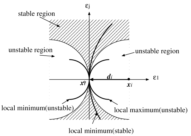
Figure 1: Stability of projection point update

When the point is a local maximum or saddle, the hypersurface is in the unstable region. However, even in the case of local minimum, there exist an unstable region, when the hypersurface is stronglly curved. We can avoid the undesired behavior by slowing down. For example, first $c_{2},\ldots,c_{m}$ and $\lambda$ are estimated from $\nabla f$ and $\nabla^{2}f$ values at the current estimate, and then if $c_{j}<|\lambda|$ for all $j=2,\ldots,m$, the point is to be local minima, then the movement $\hat{\mbox{\boldmath$x$}}_{i}^{[l+1]}-\hat{\mbox{\boldmath$x$}}_{i}^{[l]}$ to the axes in which $c_{j}<-|\lambda|$ should be shrinked by multiplying some factor $0<e_{j}<|\lambda|/|c_{j}|$.

This computationally intensive treatment would be usually necessary only after the several steps, because it is considered that the unstablity for local minima occurs a small region relatively to the size of $\mbox{\boldmath$d$}_{i}$.

3.5 Projection of the hyperplane

The update of $\hat{\mbox{\boldmath$x$}}_{i}$ causes another problem: We assumed in section 3.2 that $\omega$ and $\hat{\omega}$ have the same bases. However, $\hat{\omega}$ has bases based on the old $\hat{\mbox{\boldmath$x$}}_{i}$, while we need the new $\omega$ based on the new $\hat{\mbox{\boldmath$x$}}_{i}$. To solve that problem, $\hat{\omega}$ is projected into new bases, i.e., from the old one $\hat{\omega}^{\mathrm{old}}=\sum_{i\in\mathrm{S.V.}}\{\hat{a}^{\mathrm{old}}_{i}\phi(\hat{\mbox{\boldmath$x$}}_{i}^{\mathrm{old}})+\hat{\mbox{\boldmath$b$}}^{\mathrm{old}}_{i}{}^{\mathsf{T}}\mbox{\boldmath$\psi$}(\hat{\mbox{\boldmath$x$}}_{i}^{\mathrm{old}})\}$ to a new one, $\hat{\omega}^{\mathrm{new}}=\sum_{i\in\mathrm{S.V.}}\{\hat{a}^{\mathrm{new}}_{i}\phi(\hat{\mbox{\boldmath$x$}}_{i}^{\mathrm{new}})+\hat{\mbox{\boldmath$b$}}^{\mathrm{new}}_{i}{}^{\mathsf{T}}\mbox{\boldmath$\psi$}(\hat{\mbox{\boldmath$x$}}_{i}^{\mathrm{new}})\}$. Although $\hat{\omega}^{\mathrm{new}}$ can have more bases other than S.V., we restrict the bases to support vectors to preserve the sparsity of bases.

There are several possibilities of the projection. In this paper, we use the one which minimizes the cost function

$${1\over 2}\sum_{\mbox{\boldmath$x$}\in T}\{\hat{\omega}^{\mathrm{new}}\cdot\phi(\mbox{\boldmath$x$})+\hat{f}_{0}^{\mathrm{new}}-(\hat{\omega}^{\mathrm{old}}\cdot\phi(\mbox{\boldmath$x$})+\hat{f}_{0}^{\mathrm{old}})\}^{2},$$ (18)

where $T$ is a certain set of $x$, and we use $T=$ $\{\mbox{\boldmath$x$}_{i}$, $\hat{\mbox{\boldmath$x$}}_{i}^{\mathrm{old}}$, $\hat{\mbox{\boldmath$x$}}_{i}^{\mathrm{new}}$; $i=1,\cdots,n\}$.

Minimizing (18) leads to a simple least square problem, which can be solved by linear equations. Another possibility of the cost function is $\|\hat{\omega}^{\mathrm{new}}-\hat{\omega}^{\mathrm{old}}\|^{2}$, which leads to another set of linear equations.

3.6 Overall algorithm and the convergence property

Now let us summarize the algorithm below.

Algorithm 1: Algorithm to maximize the margin in the input space  Initialization step: Let the solution of the original SVM be $a_{i}^{(0)}$ and $f_{0}^{(0)}$; let $\mbox{\boldmath$b$}_{i}^{(0)}=\mathbf{0}$ and $\hat{\mbox{\boldmath$x$}}_{i}^{(0)}=\mbox{\boldmath$x$}_{i}$.

For $k=0,1,2,\ldots$, repeat the following steps until convergence:

1. Update of $\hat{\mbox{\boldmath$x$}}_{i}$: Calculate $\hat{\mbox{\boldmath$x$}}_{i}^{(k+1)}$ by applying (12) iteratively to $\hat{\mbox{\boldmath$x$}}_{i}^{(k)}$.

2. Projection of hyperplane: Calculate $\hat{a}_{i}$, $\hat{\mbox{\boldmath$b$}}_{i}$ and $\hat{f}_{0}$ based on $\hat{\mbox{\boldmath$x$}}_{i}^{(k+1)}$ by a certain projection method from $a_{i}^{(k)}$, $\mbox{\boldmath$b$}_{i}^{(k)}$ and $f_{0}^{(k)}$ based on $\hat{\mbox{\boldmath$x$}}_{i}^{(k)}$ (sec.3.5).

3. QP step: Solve the QP problem (8) with respect to $\alpha_{i}$.

4. Parameter update: Calculate $a_{i}^{(k+1)}$, $\mbox{\boldmath$b$}_{i}^{(k+1)}$ and $f_{0}^{(k+1)}$ by (3.3) and (11).

The discriminant function at the $k$-th step is given by (2).

 

Although Algorithm 1 does not always converge to the global minimum, we can prove the following proposition concerning about the convergence of the algorithm.

Proposition 2

Equilibrium points of Algorithm 1 are critical points of the margin in the input space. The algorithm is stable, when the update rule of $\hat{\mbox{\boldmath$x$}}_{i}$ (12) is stable for all $i$ (see also Proposition 1).

This proposition can be proved basically by proposition 1 and the fact that the linearization of QP is almost exact by a small perturbation of $\omega$. As in the case of (12), we can modify the algorithm by slowing down in (3) and (12) so that the equilibrium state is stable when and only when the margin is locally optimal. However, we don’t use it in the simulation because the case that the local minimum is unstable is expected to be rare.

Another problem of Algorithm 1 is that each iteration step does not always increase the margin monotonically. Although it is usually faster than gradient type algorithms, the algorithm sometimes does not improve the solution of the original SVM at all. Because the original SVM can be seen as a special case of the algorithm, we can use some annealing technique, for example, updating temporal variables and parameters more gradually from their initial values. However, for simplicity, we use a crude method in the simulation as follows: Repeat several steps of the algorithm (5 steps in the simulation) and then choose the best solution which gives the largest estimated value of the margin.

As for the complexity of the algorithm, we need $O(m^{2}n^{2})$ space and $O(m^{3}n^{2})$ time complexity to calculate temporal variables if the computation of a kernel function is $O(m)$, while the original SVM requires $O(n^{2})$ space and $O(mn^{2})$ time. Those calculation can be pararellized easily. This complexity is not so different when $m$ is comparatively small. Once the variables are calculated, the complexity for QP is just the same. Therefore, as far as the calculation for temporal variables is comparative to the QP time, the proposed algorithm is comparative to the original SVM. If the Algorithm 1 is heavy because of the large $m$, we can use a simplified algorithm as shown in the section 6.

As for the iteration of QP which is carried out usually for a few steps, since a current solution is an estimate of the solution, it may be able to reduce the complexity of the QP at the next iteration step.

4 Simulation results

In this section, we give a simulation result for artificial data sets in order to verify the proposed algorithm and to examine the basic performance. 20 training samples and 1000 test samples are randomly drawn from positive and negative distribution, each of which is a Gaussian mixture of 3 components with uniformly distributed centers $[0,1)^{2}$ and fixed spherical variance $\sigma^{2}=0.2^{2}$. The kernel function used here is a spherical Gaussian kernel with $\sigma^{2}=1^{2}$. The metric is taken to be Euclidean (i.e., $G_{i}$ is the unit matrix). Figure 2 and 3 show an example of results by the original SVM (initial condition) and the proposed algorithm (after 5 steps). In this case, the margin value increases from 0.040 to 0.096. Such a simulation is repeated for 100 sets of samples with different random numbers.

The estimated margins in the input space for the original and proposed algorithm is shown in figure 4 (log-log scale). By the crude algorithm described in the previous section, there are 4 cases among 100 runs that cannot improve the margin of the original SVM. The ratios of the margin are distributed from 1.00 (no improvement) to 27.9.

The misclassification errors for test samples is shown in figure 5. The ratios of error distributed between [0.40(best),1.37(worst)].

This results indicates that the margin in the input space is efficient to improve the generalization performance in average, but there are cases that cannot reduce the generalization error even when the margin in the input space increases.

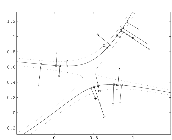
Figure 2: Result of the original SVM (margin .040). Circles ($\circ$) and crosses ($\times$) are positive and negative samples. Squares ($\Box$) represent estimates of the projection of the points by applying (12) for 10 steps.

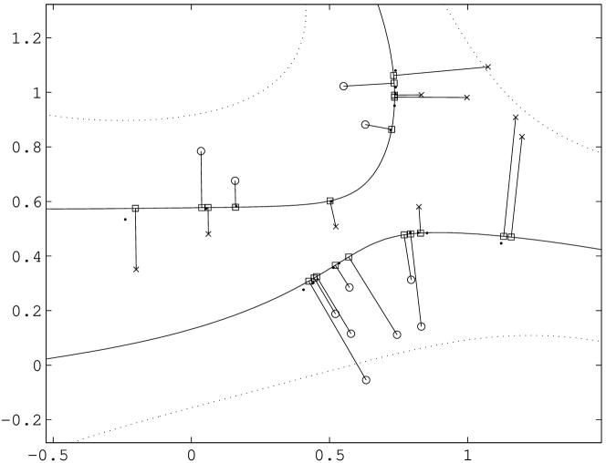
Figure 3: Result of the algorithm 1 (after 5 steps, margin .096) for the same data set as fig.2

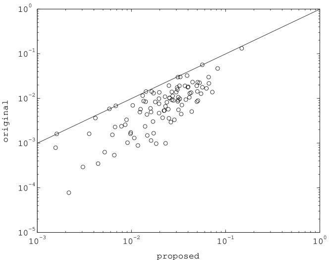
Figure 4: Margin comparison with the original SVM for 100 runs (log-log scale)

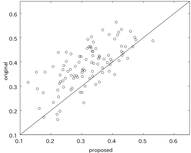
Figure 5: Test error comparison with the original SVM for 100 runs

5 Soft margin

For noisy situation, the hard margin classifier often overfits samples. There are several possibitilities to incorporate the soft margin, here we give a simple one. The soft margin can be derived by introducing slack variables $z_{i}$ into the optimization problem. If we use a soft constraint in the form

$$\omega\cdot[y_{i}\ \{\phi(\hat{\mbox{\boldmath$x$}}_{i})-\mbox{\boldmath$\psi$}(\hat{\mbox{\boldmath$x$}}_{i})^{\mathsf{T}}\hat{\mbox{\boldmath$d$}}_{i}\}-\hat{\eta}_{i}]\geq\hat{g}_{i}-f_{0}y_{i}-z_{i},$$ (19)

and adding penalty for the slack variables,

$${1\over 2}\omega\cdot\omega+C\sum_{i}z_{i},$$ (20)

By this modification, only the constraint (9) for $\alpha_{i}$ is changed to

$$0\leq\alpha_{i}\leq C,\qquad\sum_{i}y_{i}\alpha_{i}=0,$$ (21)

which is the same constraint as the soft margin of the original SVM. However, the geometrical meaning of (19) in the space is not clear. It is a future work to introduce a natural soft constraint in the input space.

6 Simplified algorithm for a high dimensional case

Although Algorithm 1 achieves the precise solution, the computation costs is high for large dimensionality of inputs. In this section, we give a simplified algorithm.

If we don’t update $\hat{\mbox{\boldmath$x$}}_{i}$, the first and the second steps of Algorithm 1 is not necessary any more. This simplification makes Algorithm 1 a little simpler because all $\hat{\mbox{\boldmath$d$}}_{i}$ terms vanish. However, let us consider further simplification.

We have shown the relation to the original SVM: the original SVM can be derived $\hat{g}_{i}=1$ and $\hat{\eta}_{i}=0$. Since $\hat{\eta}_{i}$ causes many temporal variables, we only maintain $\hat{g}_{i}$. Then all the terms related to $\hat{\mbox{\boldmath$b$}}_{i}$’s vanish.

Consequently, the above simplifications lead to the algorithm much like the original SVM. In fact, the existing code for the original SVM can be used as follows:

For each step, first $\hat{g}_{i}$ is calculated,

$$\hat{g}_{i}={\|\sum_{j}a_{i}\mathbf{k}_{x}(\mbox{\boldmath$x$}_{i},\mbox{\boldmath$x$}_{j})\|_{G_{i}^{-1}}\over\sqrt{\sum_{j,k}a_{j}^{(k)}a_{k}^{(k)}\mathrm{k}(\mbox{\boldmath$x$}_{j},\mbox{\boldmath$x$}_{k})}}.$$ (22)

Then, by letting the $(i,j)$ element of kernel matrix be $\mathrm{k}(\mbox{\boldmath$x$}_{i},\mbox{\boldmath$x$}_{j})/\hat{g}_{i}\hat{g}_{j}$, the original SVM for this kernel matrix gives the solution for each step of the simplified algorithm.

7 Conclusion

We have proposed a new learning algorithm to find a kernel-based classifier that maximizes the margin in the input space. The derived algorithm consists of an alternating optimization between the foot of perpendicular and the linear coefficient parameters. Such a dual structure appears in other frameworks, such as EM algorithm, variational Bayes, and principal curve.

There are many issues to be studied about the algorithm, for example, analyzing the generalization performance theoretically and finding an efficient algorithm that reduces the complexity and converges more stably. It is also an interesting issue to extend our framework to other problems than classification, such as regression[1, 8, 7].

In this paper, we have assumed that the kernel function is given and fixed. Recently, several techniques and criteria to choose a kernel function have been proposed extensively. We expect that those techniques and much other knowledge for the original SVM can be incorporated in our framework. Applying the algorithm to real world data is also important.

References

• [1] S. Akaho, Curve fitting that minimizes the mean square of perpendicular distances from sample points, SPIE Vision Geometry II (also found in Selected SPIE Papers on CD-ROM, 8, 1999), 237–244 (1993)
• [2] S. Amari, Differential Geometrical Methods in Statistics, Springer-Verlag (1984)
• [3] C. Cortes and V.N. Vapnik, Support vector machines, Machine Learning, 20, pp. 273–297 (1995)
• [4] D. DeCoste and B. Schölkopf, Training invariant support vector machines, Machine Learning, 46(1), pp. 161–190 (2002)
• [5] T. Hastie and W. Stuetzle, Principal curves, Journal of the American Statistical Association, 84(406), pp. 502–516 (1989)
• [6] T.S. Jaakkola and D. Haussler, Exploiting generative models in discriminative classifiers, NIPS 11, pp. 487–493 (1998)
• [7] K.R. Müller, S. Mika, G. Rätch, K. Tsuda, B.Schölkopf, An Introduction to Kernel-Based Learning Algorithms, IEEE Trans. on Neural Networks, 12, pp. 181–201 (2001)
• [8] N. Otsu, Karhunen-Loeve line fitting and a linearly measure. In IEEE Proc. of ICPR’84, pp. 486–489 (1984)
• [9] J.O. Ramsey, B.W. Silverman, Functional Data Analysis, Springer-Verlag (1997)
• [10] P.Y. Simard, Y.A. Le Cun, J.S. Denker, B. Victorri, Transformation Invariance in Pattern Recognition – Tangent Distance and Tangent Propagation, in Neural Networks: Tricks of the Trade, G. Orr and K.-R. Müller, eds., Springer-Verlag, vol.1524, pp.239–274 (1998)
• [11] K. Tsuda, M. Kawanabe, G. Rätsch, S. Sonnenburg, K.R. Müller, A New Discriminative Kernel from Probabilistic Models, NIPS 14 (2001)
• [12] V.N. Vapnik, The Nature of Statistical Learning Theory, Springer-Verlag (1995)