Complex Tilings

Abstract

We study the minimal complexity of tilings of a plane with a given tile set. We note that every tile set admits either no tiling or some tiling with $\mathcal{O}(n)$ Kolmogorov complexity of its $(n\times n)$-squares. We construct tile sets for which this bound is tight: all $(n\times n)$-squares in all tilings have complexity at least $n$. This adds a quantitative angle to classical results on non-recursivity of tilings – that we also develop in terms of Turing degrees of unsolvability.

Keywords: Tilings, Kolmogorov complexity, recursion theory

1 Introduction

Tilings have been used intensively as powerful tools in various fields such as mathematical logic (see, e.g., [Borger Gradel Gurevich 96] and references within), complexity theory [Gurevich 91, Levin 86], or in physics for studying quasicrystals (see for instance the review paper [Ingersent 91]). In all of these branches the ability of tile sets to generate “complicated” tilings is essential — it was already clear in Wang’s original papers [Wang 61, Wang 62].

A tile is an unit square with colored edges (each of the four sides has some color). Assume that a finite set $\tau$ of tiles is given. We want to form a $\tau$-tiling, i.e., to cover plane with translated copies of tiles from $\tau$ in such a way that adjacent tiles have a common edge which has the same color in both tiles.

Tiles placed in the plane can be seen as a dual view of crosses on a grid. A cross in a grid is a combination of four (colored) edges sharing a corner. Given a set of allowed crosses, one may wish to color all edges of a grid in such a way that all crosses are allowed. This question is equivalent to the original one. (Turning each edge orthogonally around its own center turns the grid of edges into its dual graph and tiles into crosses and vice versa.) Thus, one can use either representation for best visual advantages.

We call a palette a finite set of tiles that can be used to tile the plane (+palette for crosses). The problem to know whether a set of tiles is or is not a palette, is the so-called domino problem.

In order to prove its undecidability left open in [Wang 61, Wang 62], Berger [Berger 66] constructed an aperiodic set of tiles, i.e., a palette $\tau$ such that all $\tau$-tilings are aperiodic (no translation keeps them unchanged) (see also [Robinson 71] and [Allauzen Durand 96]).

Hanf in [Hanf 74] (for the origin constrained case) and then Myers in [Myers 74] (for the general case) have strengthened this result and constructed a palette that has only non-computable (non-recursive) tilings.

The aim of this paper is to understand how “complexity-demanding” a palette can be, and we measure the complexity of a palette by the minimal Kolmogorov complexity of tiling it can form. More specifically, we measure the complexity of regions in the simplest tiling that can be formed (a formal definition is given in the next section).

Some information about the complexity of tiling from the recursion-theoretic viewpoint is also provided (section 11).

What can be said about Kolmogorov complexity of a tiling? Tiling is an infinite object, so we look at $(n\times n)$-squares and measure their Kolmogorov complexity.

Item 1 of Theorem 1 below states that for each palette there exists a tiling such that complexity of its $(n\times n)$-squares is $\mathcal{O}(n)$. This bound is tight: item 2, our main result, constructs a palette $\tau$ that has only complex tilings: in each tiling, every $(n\times n)$-square has complexity at least $n$. The construction is rather complicated and is based on Berger’s construction in [Berger 66] and its further developments.

If $\tau$ is a palette with all tilings of at least linear complexity, then all $\tau$-tilings are aperiodic and non-computable because for every computable (a fortiori periodic) tiling, the complexity of its centered $(n\times n)$-squares is $\mathcal{O}(\log n)$.

Note that the right question is “what is the minimal complexity of a $\tau$-tiling” (for a given palette $\tau$) but not “what is the maximal complexity of a $\tau$-tiling”. Indeed, the maximal complexity could be large for a trivial $\tau$ such as the set of all tiles having black and white edges where random tiling has complexity $\Omega(n^{2})$.

Theorem 1 uses the same idea of embedding computations into tilings that was used to construct palette that has only non-computable tilings ([Hanf 74, Myers 74]). However, in our case we need embedding that is “dense” enough, and its construction (in non-constrained case) requires additional efforts.

It seems likely to one of us that Kurdiumov-Gacs hierarchical cellular automata (see, e.g., [Gacs 01]) could be used instead of Berger’s square hierarchy. This way a stronger result (allowing a constant fraction of missing tiles in random places) might possibly be achieved. We, however, are confident in our inability to use these (enormously complex) constructions and, in any case, the simplicity of the structure we propose has independent merits.

A more structural approach can be used to handle the complexity of tilings: a palette can always form “quasiperiodic” tilings (see [Durand 99]). We can measure the regularity of quasiperiodic tiling by the growth of the function assigning to an integer $n$ the minimal “window” size in which all patterns smaller than $n\times n$ must appear (for every position of the window and for all patterns that appear somewhere in the tiling). This approach was further developed in [Cervelle Durand 00].

Theorem 1 also implies lower and upper bounds for the number of different $(n\times n)$-squares in a tiling (Corollary 1).

Let us make some remarks about the complexity of tilings from the viewpoint of hierarchy of Turing-degrees of unsolvability. Hanf and Myers result in [Hanf 74, Myers 74] says that some palettes can generate only non-recursive tilings (i.e., of degree $>0$). This cannot be improved significantly: we cannot find a palette for which all tilings are, say, $0^{\prime}$-hard, since for every palette $\tau$, and undecidable set $A$, there exists a $\tau$-tiling $T$ such that $A$ is not Turing-reducible to $T$. This result is a corollary of classical results in recursion theory because the set of all tilings with a given palette is a $\Pi^{0}_{1}$-set (see Odifreddi book p.508 [Odifreddi 89] and references within). However, we present (see Proposition 3) a short direct proof of this fact (that goes back to Albert Muchnik and Elena Dyment and was communicated to us by Andrei Muchnik [Muchnik 00]).

2 The Main Results

There are several versions of Kolmogorov complexity $\mbox{\bf K}(x)$ expressing “the minimal description length” (see [Li Vitanyi 97]). For our purposes it does not matter which of them we use.

Theorem 1

1. For each palette $\tau$, there exists a $\tau$-tiling in which all $n\times n$ squares $n$ have complexity $\mathcal{O}(n)$.

2. There exists a palette $\tau$ such that in every $\tau$-tiling all $n\times n$ squares have complexity $\geq n$.

(The second part can be slightly generalized. A pattern on a connected subset $P$ of a tiled planar grid is the list of tiles in $P$ and their coordinates relative to the center of $P$. We encode all objects $x$ in binary denoting their length as $\|x\|$. In Theorem 1.2 we can replace $n\times n$ squares by patterns of diameter $n$.)

Item 1 of this Theorem and the following Corollary are proven in section 3. The proof of item 2 involves several constructions and will be split into several parts. Section 4 considers the easier origin-constrained case. Section 5 describes aperiodic tilings used as a background in the rest of the proof. Section 6 explains the general structure of the computation embedded in a tiling; Section 8 considers computational power of stripes (modules of different ranks that interact during the computation). Finally, section 9 considers the communication between stripes and explains how all the stripes working in parallel achieve the declared goal (preventing low-complexity fragments from appearing in the tiling).

Corollary 1

Let $D_{n}(\alpha)$ be the number of different $n\times n$ squares that appear in tiling $\alpha$.

1. Each palette $\tau$ has a $\tau$-tiling $\alpha$ such that $D_{n}(\alpha)=2^{\mathcal{O}(n)}$.

2. There exists a palette $\tau$ such that $D_{n}(\alpha)\geq 2^{n}$ for every $\tau$-tiling $\alpha$ and every $n$.

(See section 3 for the proof.)

Theorem 1 has a finitary version that says, informally speaking, that (for some palette) a pattern $x$ whose complexity is less than its diameter $d$ cannot appear in a $N\times N$-square where $N$ is the polynomial of the time needed to establish that $\mbox{\bf K}(x)<d$.

Let $U:p\to x$ be the universal algorithm defining Kolmogorov Complexity $\mbox{\bf K}(x)$ of $x$ as the minimal length of its co-image $p$. Let $U^{\prime}(p)=(U(p),\|p\|)$ enumerate the super-graph of K. Let $T_{k}(x)$ be the optimal inversion time of $U^{\prime}$ on $(x,k)$ and $S_{k}(x)$ be the minimal space $U(p)$ needs to compute each digit of $x$ from some $p\in\{0,1\}^{k}$.

Theorem 2

1. Every palette $\tau$, for each $N,k\geq\mbox{\bf K}(N)+O(1)$, has $\tau$-tiled $N\times N$ squares $x$
   with $\mbox{\bf K}(x)\leq k$ and $S_{k}(x)=O(N)+S_{k}(N)$.

2. There exists a palette $\tau$ such that no pattern $x$ of diameter $d>\mbox{\bf K}(x)$ can be extended to a $\tau$-tiled square of diameter $T_{d}(x)^{5}$.

See Section 10 for the proof.

3 Proof: the Upper Bound (Theorem 1.1)

• Proof of the upper bound.

  Fix a palette $\tau$. A border coloring $b$ of a $(n\times n)$-square assigns colors to $4n$ tile sides on the square border. A border coloring $b$ is called consistent if it can be extended to a tiling of the entire $(n\times n)$-square, i.e., there exists a tiling of $(n\times n)$-square that matches $b$. Consider the following algorithm that, applied to a consistent border coloring of a square of size $n\times n$ where $n=2^{k}$, extends it to the tiling of the entire square:

  A. Find the alphabetically first coloring of the central lines dividing the square into four equal squares such that all four squares get a consistent border coloring.

  B. Apply the algorithm recursively to four border colorings of smaller squares. (For $(1\times 1)$-square consistent border coloring is just a tile coloring.)

  When this algorithm is applied to a square with side $2^{k}$, it generates a tree of recursive calls for sub-squares with sides $2^{l}$ for all $l$ (“standard” sub-squares). On each standard sub-square the complexity of tiling is proportional to square side (since tiling is computed by our algorithm starting from border coloring).

  Each non-standard sub-square with side $m$ is contained in $4$ standard sub-squares with sides smaller than $2m$ and therefore has complexity $\mathcal{O}(m)$. This argument shows that for some constant $c$ and for all $k$ there exists a tiling of size $2^{k}\times 2^{k}$ such that all $(m\times m)$-sub-squares in this tiling have complexity at most $cm$.

  Using compactness argument, we conclude that there exists an infinite tiling with the same property.

  (Here are the details. For a fixed $c$ let us call a tiling of $(n\times n)$-square good if all $(m\times m)$-subsquares of it have complexity at most $cm$. As we have seen, for some $c$ there exist good $(n\times n)$-tilings for arbitrarily large $n$. Call a tiling of $(n\times n)$-square extendible if it appears as a central part of some good tiling of arbitrary large size. Note that each extendible tiling can be extended to some extendible tiling of $(n+2)\times(n+2)$-square by adding one more layer. Continuing this process, we get a tiling of the entire plane.) $\square$

• Proof of the Corollary. The first statement of Corollary 1 is a direct consequence of upper bound in Theorem 1, since the number of different objects with complexity $\mathcal{O}(n)$ is $2^{\mathcal{O}(n)}$.

  To prove the second statement we use the lower bound from Theorem 1. Let $\tau$ be the palette such that all $\tau$-tilings have complexity at least $5k$ for $(k\times k)$-squares. (We have weaker bound $k$ in Theorem 1, but it does not matter since we can combine several tiles into one larger tile.)

  Let $\alpha$ be a $\tau$-tiling. Assume that for some $n$ the number of $(n\times n)$-squares in $\alpha$ is less than $2^{n}$. Consider a square of size $k\times k$ where $k$ is a large multiple of $n$, and its “border” formed by $(n\times n)$-squares. Since each border square can be described by $n$ bits (there are less than $2^{n}$ of them), the whole border has complexity approximately $4k$ (for large $k$). Then we can change the tiling, replacing the interior of $(k\times k)$-square by the alphabetically first tiling that is compatible with the border. Then new interior is determined by the border, therefore the complexity of new $(k\times k)$-square is less than $5k$ and this contradicts to our lower bound (that is valid for all tilings). $\square$

4 Proof: Origin Constrained Case

To prove the lower bound, we start with the much simpler “origin constrained case”. It means that we consider only those tilings of the plane that have a fixed tile at the origin. This allows us to enforce the tiling to be a time-space diagram of a Turing machine.

4.1 Computation Performed

Let us agree that each horizontal line in a tiling represents a Turing machine’s tape at time $t$ where $t$ is the vertical position of that line. The tile used at position $(x,t)$ encodes the contents of cell number $x$ at time $t$ (including the head state if the head is inside cell $x$ at time $t$).

The rules of Turing machine are local and therefore can be encoded in terms of tilings (one may represent overlapping groups of cells on time-space diagram by a tile). This technique is well known (see, e.g., [Wang 61]) and we won’t go into details here. It works only for constrained case; we require the origin to be the tile that contains head of TM, otherwise a tiling may contain no computation.

Since tilings can simulate the behavior of a TM with an infinite tape, it remains to construct a TM that will ensure high complexity of its time-space diagram.

Imagine that we have a TM with a double tape: each cell is the Cartesian product of a workspace and an “input bit”. The TM may change only the workspace of each cell, the input bit is read-only. This TM can checks that input sequence is “complex enough”, that is, its input string has Kolmogorov complexity at least $ck$ for a constant $c<1$ in each $k$ consecutive columns. More precisely, the set of all finite strings with low Kolmogorov complexity is enumerable (we can try all the programs in parallel and look for the cases when the output of a program is significantly longer than the program itself). Our TM can enumerate such simple finite strings, compare them with segments of the input tape, rejecting the tiling if any match is found.

This addresses Theorem 1.2 for patterns of width (equal to the number of input bits) close to their diameter. For narrow patterns we must superimpose two orthogonal copies of this construction. This suffices, since diameter of any pattern equals, within a factor of 2, to either its width or height.

We need now to prove existence of sequences our machine does not reject.

4.2 Complexity Lemma

Lemma 1

For each $c\!<1$ there exists a binary sequence $\omega$ with $\mbox{\bf K}(x)\geq c\|x\|-\mathcal{O}(1)$ for all its substrings $x$.

Remark 1. For our purposes it is enough to prove this lemma for some positive $c$ (however small). Still, the more general statement (for all $c<1$) is of some independent interest, so we prove it in this stronger form. We cannot strengthen this Lemma further since for each sequence $\omega$ the above inequality fails for some $c<1$ and an infinite set of substrings of unbounded lengths. (If every binary string is a substring of $\omega$, then this is evident. If some string $X$ does not appear in $\omega$, then the bound $\mbox{\bf K}(x)\leq c\|x\|+\mathcal{O}(1)$ is true for some $c$ and for each substring $x$ of $\omega$.)

Remark 2. It is not important which version of complexity to use in the lemma since $c$ is not fixed and all versions differ by a logarithmic term. However, in the proof it is convenient to use prefix complexity.

Remark 3. In this lemma we speak about sequences that are infinite in one direction (though the sequence of indices on the tape is bi-infinite). However, this is not important: if there exists an infinite in one direction sequence with this property, there are arbitrary long finite sequences with this property, and the standard compactness argument shows that there are bi-infinite sequences with this property.

[In fact, compactness is not even needed here. We can construct a bi-infinite sequence with this property from a one-way infinite one by putting bits alternatively left and right at the small cost of a multiplicative factor 2 on $(1-c)$.]

Thus our lemma proves that the above constructed TM does not halt for some input sequences (having this property).

• Proof of Lemma 1.

  Let us prove first for some constants $c^{\prime},c^{\prime\prime}$ that for every string $x$ and natural number $n$ there exists an $n$-bit string $y$ such that

  $$\mathit{\mbox{missing}}{KP}(xy)+\mathit{\mbox{missing}}{KP}(n)+c^{\prime}\geq\mathit{\mbox{missing}}{KP}(\langle x,y\rangle)+c^{\prime\prime}\geq\mathit{\mbox{missing}}{KP}(x)+n$$

  Here $\langle x,y\rangle$ stands for the encoding of the ordered pair formed by $x$ and $y$. The second inequality is true since of $2^{n}$ such pairs with a given $x$ some must have a universal semimeasure smaller than $x$ at least by a factor of $2^{n}$ and thus an $n$ bits higher complexity.

  And the first inequality is true since $\langle x,y\rangle$ can be reconstructed from $xy$ and $\|y\|=n$.

  Now we can prove the lemma as follows. For a given $c<1$ we choose $m$ such that

  $$m-\mathit{\mbox{missing}}{KP}(m)-c^{\prime}\geq cm.$$

  Then, starting with an empty sequence, we add blocks of length $m$ to it in such a way that each block increases the complexity at least by $cm$. Adding several blocks, we increase the length by some $M$ (which is a multiple of $m$) and the complexity at least by $cM$. Since

  $$\mathit{\mbox{missing}}{KP}(uv)\leq\mathit{\mbox{missing}}{KP}(\langle u,v\rangle)+O(1)\leq\mathit{\mbox{missing}}{KP}(u)+\mathit{\mbox{missing}}{KP}(v)+c^{\prime\prime\prime},$$

  the group of added blocks has complexity at least $cM-c^{\prime\prime\prime}$. Thus we have proved our Lemma for segments that start and end at coordinates that are multiples of $m$. The boundary effects can be compensated by a small change in $c$. $\square$

5 Proof: Self-similar Pattern

Now we have to consider the general case, no more requiring a fixed tile at the origin. Let us start with some informal remarks. The palette must prevent individual tilings from being periodic. This can be provided by a “self-similar” structure: tiling is divided into “mega-tiles” — blocks of large sizes (squares of size $2^{n}\times 2^{n}$ for all $n$) that behave like individual tiles.

A self-similarity of this type was used in Robinson’s construction of an aperiodic tiling (see Robinson’s original paper [Robinson 71] and an exposition given in [Allauzen Durand 96]). A slightly more rigid construction (where all “mega-tiles” are aligned, which was not the case for Robinson’s palette), is explained in [Levin 04] and [Durand Levin Shen 04]. We do not repeat the latter construction here but just describe the self-similar pattern that can be enforced by it.

Consider a grid of $2\times 2$ squares separated by two cells (Fig. 2).

Then group these squares into groups of four squares whose centers form a twice larger square (Fig. 2). We get a rank 2 grid formed by $(4\times 4)$-squares separated by four cells; this grid is twice larger than the rank 1 grid.

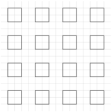
Figure 1: Rank 1 squares

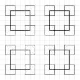
Figure 2: Rank 2 squares

Then we group rank 2 squares into groups of four squares whose centers are corners of rank 3 square etc. We will refer to the edges on the borders of squares of all ranks as dark. (Fig. 3 shows one rank 4 square and underlying hierarchy of smaller squares.)

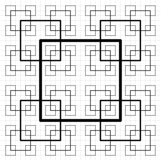
Figure 3: Hierarchy of squares

Note that we have described not one specific pattern but an uncountable family of patterns: at each rank we have a two-bit choice while grouping squares into 4-groups. Therefore, a pattern (together with a specified cell in it) is determined by an infinite sequence of bits.

Note also that the dark pattern may be either connected or not. The latter happens if there exists a “separating line” (a vertical or horizontal line that does not intersect any dark square). The dark pattern in these cases has $2$ or $4$ connected components separated by either a horizontal or vertical line, or by an infinite cross. For the case of one separating line we require it to be of uniform color (either light or dark). For the case of two separating lines they must form a dark corner (four possible orientations).

Looking at some non-separating line, we see that it consists of alternating dark and light segments of length $2^{k+1}$ where $k$ is the rank of dark squares adjacent to it. We say that this line has rank $k$ (is a $k$-line).

We assign infinite rank to separating lines. The non-connected case (when separating lines exist) is called the degenerated case in the sequel and requires special treatment, see Subsection 9.5.

Proposition 1

There exists a palette and a projection of its colors into $\{\text{dark},\text{light}\}$ such that every tiling is projected onto some pattern of the described type.

See [Levin 04] and [Durand Levin Shen 04] for the proof. This palette $P$ (+palette, actually) provides two orientation bits which will help us below. These bits on each edge $x$ show vertical and horizontal direction to the nearest center of the dark square with border co-linear to $x$. These bits form distinct crosses at the intersections of lines of the same rank, of adjacent ranks, and of more distant ranks. In a more informal language (that will be used in the sequel) one can say that each edge on a dark square “knows” (i.e., this information is encoded in its color) whether it belongs to the left or to the right half of the square. The same is true for the lower and upper half of the square (and vertical edge). The corner node “knows” (i.e., this information is encoded in the neighbor colors) that it is a corner node, etc.

To provide more formal description of the pattern, it is convenient to use a kind of $2$-adic coordinates. Consider lines that go in-between $2\times 2$ squares (one line per four cells). Taking them as reference lines, we provide “modulo $4$” coordinates, or just $4$-coordinates, as shown in Figure 5.

The same can be done modulo $8$ for rank $2$ squares, as shown in Figure 5.

Figure 4: $4$-coordinates and rank $1$ squares

Figure 5: $8$-coordinates and rank $2$ squares

Note that $8$-coordinates are consistent with $4$-coordinates (two last bits of the $8$-coordinate form the $4$-coordinate). We can then consider $16$-coordinates, $32$-coordinates etc. They extend each other, and for each point of the grid we get a $2$-adic coordinate that is an infinite (to the left) sequence of bits.

Vertical sides of rank $k$ squares have $x$-coordinates $\ldots 10^{k-1}$; the same is true for $y$-coordinates of horizontal sides. So we can assign rank to vertical and horizontal lines ($1$ plus the number of zeros at the end of their coordinates). Lines of rank $k$ contain sides of rank $k$ squares. Each line has some uniquely defined rank, except for the line with zero coordinates. This line can exist or not depending on the pattern (this is the separating line we mentioned above).

The centers of rank $k$ squares have coordinates that end with $k$ zeros, i.e., lie on the rank $(k+1)$ lines. Other features of the pattern can be also easily expressed in terms of coordinates. For example, a vertical grid line with coordinate $x$ intersects (the interior of) rank $k$ squares if and only if last $k+1$ digits of $x$ belong to the open interval $(010^{k-1},110^{k-1})$.

6 Proof: Stripes and Grids

Let us start with some informal remarks. The high complexity of tilings comes from an input sequence $I$, horizontal and infinite in both directions. Each bit occupies a vertical line. A Turing Machine (TM) verifies that $I$ has no low complexity segments. This computation represented by tilings as space-time diagrams.

As it was done for the origin-constrained case, the configuration of a TM (the contents of its tape including the head position) is represented by colors of horizontal edges. Their shifts in the vertical direction represent time evolution. The consistency of states in subsequent moments of time is achieved via vertical edges that carry the state information from one horizontal line to another. The correctness of state transitions is assured by a palette that restricts the coloring of crosses of these vertical and horizontal lines.

In the origin-constrained case the whole tiling represented one computation. Now, instead, we arrange infinitely many coexisting and interacting computations. It is not a problem to combine two computations at the same location: the Cartesian product of two finite alphabets is still finite. But this cannot be done for infinitely many computations. Instead, they are separated in space and time so that each edge is used only by a limited number of them. All the computations should then communicate with each other to check that every substring of the input sequence has high complexity.

The organization of these processes “formats” the plane using the self-similar Block Pattern (described above). This formatting is used to arrange space for infinitely many “computations”. Each computation is performed by a subgrid that consist of finite number of (infinite) vertical lines and infinite number of (finite) horizontal lines arranged as in Fig. 6. Their intersection points are called nodes of the subgrid.

Figure 6: Subgrid for one computation

Each horizontal line is divided by nodes into segments ($s_{1},\ldots,s_{n}$). Each segment carries one symbol of TM tape or the state of one cell in the cellular automaton. The changes happens in nodes only (both for horizontal and vertical lines). All this can be:

• organized locally if each edge of the subgrid knows its place in the subgrid (whether it is at the node, lies on the left/right boundary, or between nodes, etc.).

• used in a usual way to simulate computations of TM (or cellular automata) with the tape of fixed size.

Note that the “physical” distances between the grid lines can be arbitrary, they do not affect at all the computation performed on the grid. (In fact all the vertical distances will be the same, but not the horizontal distances. This is somehow shown in Figure 6.)

Note also that the edges included in the grid do not know how far they are from the nodes they connect (it is not needed and also there is not enough colors to encode this).

Now we describe how the subgrids are localized. Let us introduce some terminology. Each dark square of rank $k$ is included in a twice larger $k$-block. For each $k$, the plane is split into $k$-blocks. A bi-infinite column of vertically aligned $k$-blocks forms a $k$-stripe (see Fig. 8).

The borderlines between $k$-blocks have $2$-adic coordinates that end with $k+1$ zeros.

Each $k$-stripe is a union of two $(k-1)$-stripes, called its children (see Fig. 8). (For example, $3$-stripe $[\ldots 00000,\ldots 10000]$ that lies between vertical lines with coordinates $\ldots 00000$ and $\ldots 10000$ is the union of two $2$-stripes: the left is $[\ldots 00000,\ldots 01000]$, the right is $[\ldots 01000,\ldots 10000]$.

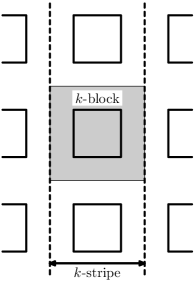
Figure 7: Grid of $k$-blocks and $k$-stripe

Figure 8: Stripe and its two children

We provide for each stripe a subgrid that is located inside the stripe. (This subgrid hosts a computation that is finite in space but infinite in time.) These computations are not completely independent: each computation communicates with its parent computation (located in the parent stripe) and its two children computations (located in children stripes). The communication is implemented by sharing some vertical lines, communication lines. There are three communication lines in each subgrid: the center line and the vertical lines that contain the vertical side of $k$-square; the latter two lines are the leftmost and rightmost lines in the subgrid and are called “border lines”.

Note that the center line of $k$-square is at the same time the border line for the $k+1$-level subgrid. Using the center line, $k$-computation can communicate with its parent $(k+1)$-computation, and using the border lines, $k$-computation can communicate with its two children $(k-1)$-computations.

We need also to specify the other vertical lines that are included in the $k$-level subgrid. They are called $k$-channels and lie between the border lines (see below about their exact location). The horizontal lines of the subgrid, called $k$-tapes in the sequel, are just bottom lines of $k$-squares (see Fig. 9).

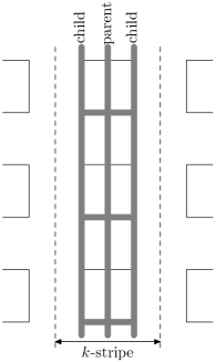
Figure 9: Horizontal and some vertical subgrid lines for a $k$-stripe

7 Designation of $k$-channels

Designating $k$-channels, we should have in mind that:

(1) Each vertical line should be shared by a limited number of computation subgrids (in fact, three in the construction explained below: it can be a communication line in two subgrids and a channel in the third one).

(2) There should be sufficiently many $k$-channels to provide enough space for the computation performed by a subgrid. (In our construction the $k$-level subgrid has $\Theta(2^{k/2})$ vertical lines, which is about the square root of its geometric size.)

(3) Each node should know its role in every subgrid it belongs to. (Since the number of subgrids is limited, this is a finite amount of information that can be encoded in the finite number of colors. What is important, we need the correct information be enforced by local rules.)

Let us explain how all three goals can be achieved. First, let us agree that we have two types of dark squares, say, red and blue squares, and the colors alternate (so $2k$-squares are red and $(2k+1)$-squares are blue or vice versa). This is very easy to arrange: an additional bit distinguishes between red and blue squares, and this bit should differ for two intersecting dark squares (note that if two squares intersect, their ranks differ by $1$).

Then for a vertical line we define its color (red or blue) as the color of the square whose side it contains. Since the vertical sides of a $k$-square have coordinates $\ldots 010^{k-1}$ and $\ldots 110^{k-1}$, the color of a vertical line depends on whether the number of trailing zeros is even or odd. (The color is defined uniquely for all lines except for the separating vertical line if it exists in the pattern; the separating line can have arbitrary color.) Note that we can easily distribute the color along the line, so each point on the line knows the line color.

Now the rule:

for each line $L$ we look for the smallest square of the same color that intersects $L$ (not taking into account the square that has $L$ as its border); if this square is of rank $k$, the $L$ line is declared to be $k$-channel and belongs to the computational subgrid for the corresponding $k$-stripe.

In other terms, consider a line of rank $k$. It is a border line for $k$-squares. The construction guarantees that it is a center line for $(k-1)$-squares and does not intersect smaller squares. So we should look for squares of rank $k+2$, $k+4$ etc. until we find a square that intersects this line. (Note that rank $k$ line cannot go through the center or along the sides of those squares.)

For $2$-adic coordinates: first we find the rank of the line looking at trailing zeros. Rank $k$ means that there are $k-1$ trailing zeros, i.e., the coordinate ends with $10^{k-1}$. Then we split bits on the left into $2$-bit blocks, as shown in Figure 10. Going from right to left, we find the first block that contains $01$ or $10$ (this means that the line intersects the corresponding square).

Figure 10: Finding the square

So we see that goal (1) is achieved.

To estimate the number of $k$-channels in a given $k$-subgrid, we can either use the coordinate description or geometric argument. The coordinate description shows that we can use blocks $00$ or $11$ after the $01$/$10$ block and the trailer of the form $1\ldots 0$. This gives $2^{k/2+O(1)}$ options for $k$-squares. (For each of $k/2+O(1)$ levels we exclude two of four possible blocks $00$, $01$, $10$ and $11$, i.e., half of the lines.)

We can count also the $k$-channels for a given $k$ in a top-down fashion. Each $k$-square has two $(k-1)$-children of the opposite color and four $(k-2)$-grandchildren of the same color, see Figure 11. (This figure does not keep the vertical distances since only horizontal positions matter now.) Two grandchildren (and all their descendants) lie outside the zone of $k$-square (i.e., on the left or on the right of $k$-square). Two other provide four $k$-channels that are lines of rank $k-2$.

Figure 11: Grandchildren and their grandchildren

Each of these two grandchildren has four grandchildren; two of them are shadowed by $(k-2)$-squares (and produce $(k-2)$-channels, not $k$-channels); each of two other produces two $k$-channels, so we get $8$ $k$-channels that are lines of rank $k-4$.

We continue by induction and conclude that our $k$-square has $4^{t}$ descendants of rank $k-2t$; some of them are shadowed by squares of intermediate level (together with the whole stripe), some lie outside the zone of the initial $k$-square (together with the whole stripe), and $2^{t}$ (together with the whole stripe) are not shadowed and lie inside the zone (together with the entire stripe) producing $2^{t+1}$ $k$-channels being lines of rank $k-2t$.

So the total number of $k$-channels in the zone of some $k$-square is $4+8+16+\ldots$, and this sum has $k/2+O(1)$ terms, so it is equal to $\Theta(2^{k/2})$. The goal (2) is achieved.

For (3), let us look at some vertical line. It knows its color. Also the points where it intersects the squares of the same color are locally known. We can consider them as “brackets” (opening bracket means that line comes in the square, and closing bracket means that is goes out). So we reduce our task to the following problem: having a correct bracket structure on a line, find the innermost brackets. It is easy to do by local rules, if each brackets sends a signal in the outside direction: the innermost bracket is the bracket that does not receive that signal.

8 Proof: Computational Subgrids and their Power

Looking at a computational subgrid, we may ignore the rest of the plane as well as the geometric parameters of the embedding of this subgrid (distances between the lines etc.). For us it is just a vertical stripe that obeys some local rules (rules for the left/right boundary could differ).

Such a tiling represents the time-space diagram of a finite cellular automaton (finite number of cells that change their state depending on the previous states of themselves and of their neighbors, according to some rule which is the same for all automata except for the leftmost and rightmost one, who have special rules).

This confronts us with the problem we started with: how to initiate a computation? But now the situation is different: we work in a stripe of a finite size, so the leftmost and rightmost cells know that they are on the boundary, and this allows us to restart computation “once in an exponential while” using a counter.

This type of self-stabilization is easy to achieve. We may simulate a time-space diagram of a Turing machine. To ensure that a head of TM exists and is unique, we may require that some bit is $0$ at the left end, is $1$ at the right end, is monotonic (local rule) and the place where the bit changes behaves like a head of TM. This machine can perform counting in a positional number system adding $1$ to the counter all the time. When an overflow happens, we have to restart some other computation simulated in parallel by the stripe. If the base of our positional number system is large enough, the counting process takes more time that the other computation we simulate (if the latter computation does not repeat itself).

Let us illustrate this technique using the model example of an isolated stripe.

Consider a vertical stripe (finite in horizontal direction and bi-infinite in vertical (temporal) direction. Assume that left and right borders of the stripe have special “left” and “right” colors. We want to tile the stripe with tiles from a given tile set (respecting the border colors).

Let us assume also that all tiles of our palette are divided into two types ($0$-tiles and $1$-tiles) and tiling rules guarantee that all tiles on a vertical line have the same type. This guarantees that each vertical line in a tiling carries one bit (its type) and thus each tiling of stripe of width $w$ determines a bit string of length $w$.

So for each palette $\tau$ we get a set of strings $L_{\tau}$ that corresponds to all $\tau$-tilings of stripes (strings of length $n$ in $L_{\tau}$ correspond to the tilings of the stripe of width $n$).

Proposition 2

1. For every tile set $\tau$ the language $L_{\tau}$ belongs to PSPACE.

2. Every language $L$ that is decidable in linear space can be represented as $L_{\tau}$ for some tile set $\tau$.

• Proof. Part 1 can be proved in the same way as Savitch theorem ($\text{NPSPACE}=\text{PSPACE}$). A $\tau$-tiling of an infinite stripe exists if and only if there exists a tiling of a $w\times h$ rectangle (where $w$ is stripe width and $h\in 2^{\mathcal{O}(w)}$) that has the same colors on top and bottom lines. Indeed, rectangles with this property can be combined into a (periodic) tiling of the entire stripe. On the other hand, there is only $2^{\mathcal{O}(w)}$ possible colorings in a horizontal section, so in every tiling of an infinite stripe identical sections appear at distance at most $2^{\mathcal{O}(w)}$. Now we can write a recursive procedure that checks whether there exists a tiling of a rectangle of width $w$ and height $h$ with given top and bottom that runs in space $(w\log h)^{\mathcal{O}(1)}$ and use it to determine whether a given string of length $w$ belongs to $L_{\tau}$. (Consider sequentially all possibilities for the colors along the middle line of the tiling and for each possibility make two recursive calls for the two parts of the tiling.)

  Part 2 uses self-synchronization technique explained above: since every computation with space $\mathcal{O}(w)$ terminates in time $2^{\mathcal{O}(w)}$, we can superimpose the computation with a TM computation that keeps a $\mathcal{O}(w)$-bit integer (counter) in each horizontal line and increases it by $1$ all the time. When an overflow happens, the main computation is “rebooted” in that line. As we have mentioned, this rebooting procedure gives the main computation enough time to terminate.

  This proposition is not directly used in the proof of main theorem. It is presented here as an illustration of the self-stabilization technique used in in our main construction together with other key ingredient, the hierarchical communication between the stripes. $\square$

9 Proof: Hierarchy of Computations

We have seen that a subgrid can compute every predicate that can be computed in linear (in its effective width: $\Theta(\sqrt{N})$ for square with side $N$) space.

However, our construction of tiling with linear complexity of squares will use subgrids in a more subtle way: different computations communicate with each other and therefore become parts of some global computation. Let us explain how it is done.

9.1 Input Bits

We assume (as we have done in the constrained case) that each vertical line carries one bit (that propagates vertically). Therefore, tiling determines a (horizontal) bi-infinite sequence of bits. Our goal is to guarantee that this sequence does not contain substrings with low Kolmogorov complexity (in the same way as for origin-constrained case).

9.2 Zones of Responsibility

Recall that computation subgrid based on rank $k$ squares was located in the middle part of a stripe twice wider than the squares themselves. This stripe contains $2N$ vertical lines (and input bits) and we say that these lines and bits are in the “zone of responsibility” of this subgrid. Figure 8 shows $k$-stripe that is the zone of responsibility for a computational subgrid based on the large square in the middle; this $k$-stripe is the union of its two children who are $(k-1)$-stripes. These stripes are zones of responsibility for two computation subgrids based on the smaller squares.

For each $k$ the entire plane is divided into non-overlapping $k$-stripes that are zones of responsibility for subgrids based on $k$-squares. Each zone is divided into two children who are zones of responsibility for smaller subgrids; these zones are then divided into smaller zones etc. So we get a tree-like structure of degree $2$ whose vertices are computation subgrids. Each has two children and one parent, except for the smallest ones that do not have children.

9.3 Communication Between Stripes

Communication between parent and child subgrids is easy to organize since parent and child share some line that can be used as a meeting point for the corresponding computations (Turing machines). Of course, the heads of two machines need not to be at the same time at the meeting point, and this creates some delay.

Note that visibility of finite number of bits is enough for asynchronous communication (one of the bits can be used as “ready” flag while other are used as information bits), and the delay ($\mathcal{O}(\sqrt{N})$ steps for each transaction, if TM visits regularly the meeting points) is acceptable (see below). Therefore we assume that serial asynchronous communication between parent and its children is possible.

9.4 Bit Servers

It remains to explain what each subgrid computes. It runs in parallel (for example, using time sharing — or we can simulate two-head TM) two processes. The first process is called BitServer; the second one is called ComplexityCheck. Let us explain first what BitServer does.

It serves requests about bits in the zone of responsibility of the subgrid where it runs. Such a request contains bit address (relative to the start of the zone) of logarithmic length and should be answered by providing a value of the input bit with given address. BitServer uses the most significant bit of the address to determine to which child it should forward the remaining part of the address, and then waits until this child provides a reply (which is then sent to BitServer’s client).

This recursion stops at the lowest rank where each of $\mathcal{O}(1)$ required input bits is at $\mathcal{O}(1)$ distance from the computation, so we may assume that these bits are directly accessible.

Note that BitServer is able to provide inputs bits from the entire zone of responsibility (even outside of the physical location of the subgrid) due to its children.

9.5 Complexity Check

BitServers are useless if nobody uses them, so we need to describe the second process, ComplexityCheck. This process runs in each subgrid and tries to check whether the sequence of input bits in its zone of responsibility has no substrings with small Kolmogorov complexity (as it was done for origin-constrained case). The ComplexityCheck process gets bits from the BitServer of the same computational stripe. BitServer interleaves requests from ComplexityCheck with external requests (see “Time bounds” below).

The problem is that (compared to the origin-constrained case) each computation stripe has limited abilities: it can perform only $\sqrt{N}$-space computations to check $\mathcal{O}(N)$ bits. Therefore, each stripe should rely on higher ranks for complete check (the computation time needed to find that some string has low Kolmogorov complexity is not bounded by any computable function of string’s length).

This cooperation between ranks is indeed possible if ComplexityCheck is organized in a proper way. This process generates the list of “forbidden” string (strings with low complexity). Thus all ranks compute the same list in the same order (computation terminates when it meets time/space constraints). When a forbidden string appears in a computation it is tested against all substrings of the same length that are in the responsibility zone of the involved computation stripe. (This testing is performed by requiring bits from BitServer.) If a forbidden string is found in the input sequence, then the computation halts (making the tiling impossible).

If some string has low complexity, then it appears in the list of forbidden strings and therefore the computational stripes of sufficiently high rank will have enough time first to generate it and then to check all substrings against it.

Can we conclude now that all the substrings in the bi-infinite sequence of input bits have high complexity because they are ultimately checked in the computational stripes of all ranks? No. The problem is that the tree-like structure of computational stripes may consist of two disjoint parts that never meet. (This is a “degenerate case” discussed earlier.) But this does not hurt us because in this case each substring of the input (in the worst case) consists of two parts that are checked separately. Taking the longer part, we see that it is not forbidden and has high complexity. Therefore, every (sufficiently long) substring of input sequence has complexity at least $cn$ where $n$ is its length and $c$ is some constant. We can then increase $c$ by combining several tiles into one bigger tile.

9.6 Time Bounds

The only thing that we still have to check is that all this communication and computation can be performed in $\sqrt{N}$-space (and $\exp(\sqrt{N})$-time). Indeed, each bit address takes logarithmic space (and this is much smaller than $\sqrt{N}$-space that is available). The depth of recursion is logarithmic. So if we assume that BitServer interleaves internal requests (from ComplexityCheck of the same rank) with external requests, the time to fulfill them will be still $\exp(\mathcal{O}(\log))$, i.e., polynomial. Note also that the slowdown induced by testing a forbidden string (when it appears) against all substrings in the zone of responsibility is polynomial (in the width of the zone), while the time bound is exponential. So this slowdown does not prevent the generating process from generating every forbidden string (at a high enough rank).

This ends the proof of Theorem 1.

10 Proof: Theorem 2

• Proof. To prove Theorem 2.1, denote $s_{N}$ the space used by the algorithm of Section 3 that checks consistency of a border coloring of a square. Then $s_{2N}=s_{N}+O(N)$, and so, $s_{N}=O(N)$.

  The proof of 2.2 is essentially the same as the proof of Theorem 1 with two additions addressing minor issues. First, the self-stabilization counter of Section 8 restarts computation very rarely, with exponential intervals. Thus, a meaningless computation can run for a long time before the re-initiation. It can fail to discover low complexity of the input, and thus allow it in a large tiled square. This is easy to remedy just by restricting the counters to (sufficiently large) polynomial values. Such counters are implemented by a constant number of unary integers.

  The second issue is that $x$ may appear near the border of large $N\times N$ squares. Formally speaking, Proposition 1 says nothing about finite tilings. However, its proof (see [Levin 04, Durand Levin Shen 04]) guarantees that rank $k$ structure can be distorted only near the border of the tiled region: for each $k$ there exists some $m(k)=\mathcal{O}(2^{k})$ such that the part of tiling that is $m(k)$ tiles apart from the border, has a correct structure at rank $k$ (i.e., for $2^{k}\times 2^{k}$ squares). This can be proved by induction over $k$ since the argument in [Durand Levin Shen 04] (that shows that $1$-tiles are grouped into $2$-tiles in a regular way) uses only a small neighborhood.

  So the checking goes on in the internal part of the tiled region (square) and guarantees that the bit sequences there have no simple substrings whose simplicity can be established fast. The problem is to bring these complex bits to the border of the tiled region. This can be easily done with the following trick: let us overlap four constructions of the described type that propagate bits along the lines with direction $(2,1)$, $(2,-1)$, $(1,2)$, $(1,-2)$ instead of vertical lines that we have used for bit propagation. For every point on the border at least one of these four directions brings us in the internal part of the tiled region (square), so the bits on the border are also complex.

  $\square$

11 Turing Degrees of Tilings

In this section we are concerned with Turing-degrees of tilings; we provide a simple direct proof of the following theorem.

Proposition 3

For each palette $\tau$ and for every undecidable set $A$ there exists a $\tau$-tiling $T$ such that $A$ is not Turing-reducible to $T$.

Corollary 2

For every palette $\tau$, there exists a $\tau$-tiling $T$ such that $T$ is not $\textbf{0}^{\prime}$-hard.

• Proof. Let us consider the space $\mathcal{T}$ of all configurations made of $\tau$-tiles (both tilings and configurations with tiling errors). This space can be considered as $\tau^{\mathbb{Z}^{2}}$ and thus endowed with the product (Cantor) topology. The set $\tau$ of local rules defines a closed (compact) subset $C$ of $\mathcal{T}$ consisting of all tilings. This subset is an effectively closed subset (its complement is a union of an enumerable family of basic open sets that correspond to violations of local rules). By our assumption $C\neq\emptyset$.

  Let $M$ be some oracle machine that uses a tiling $T\in\mathcal{T}$ as an oracle. Let $x$ be some input for $M$ and $a$ be some output value for $M$ (i.e., $a=0$ or $a=1$ if we consider machines that decide some set). Consider the set of all oracles $T\in\mathcal{T}$ such that $M$ using $T$ produces answer $a$ on $x$. This set depends on $M$, $x$ and $a$; we denote it by $U(M,x,a)$. It is easy to see that $U(M,x,a)$ is an effectively open set: we have to simulate $M$ on input $x$ for all possible oracles and look for all computation branches that end with answer $a$. In this way we generate basic open sets whose union is $U(M,x,a)$.

  If $C\subset U(M,x,a)$, then $M$ produces answer $a$ on input $x$ for all $\tau$-tilings. The crucial observation: if it is the case, we can find it out eventually. Indeed, in this case the enumerable family of base open sets that form $U(M,x,a)$ and the enumerable family of base open sets that form $\mathcal{T}\setminus C$ together form a covering of compact space $\mathcal{T}$. For compactness reasons, finite number of sets are enough. Enumerating both families, we will discover this finite covering at some point.

  Now we can prove that there is no machine $M$ that reduces the undecidable set $A$ to every $\tau$-tiling. (This statement is a weak form of our theorem.) Indeed, this means that correct answer (we denote it by $A(x)$) is produced for every input $x$ and every oracle $T\in C$, i.e., $C\subset U(M,x,A(x))$ for all $x$. But then we can compute $A(x)$ without oracle by looking for all $a$ such that $C\subset U(M,x,a)$. The correct value $A(x)$ will be found; no other one can appear since $U(M,x,a)$ and $U(M,x,a^{\prime})$ are disjoint when $a\neq a^{\prime}$.

  The next step is to use diagonal argument and find $\tau$-tiling $T$ such that no machine decides $A$ using $T$ as an oracle. Let $M_{1},M_{2},\dots$ be the enumeration of all (oracle) machines. We construct a sequence

  $$C_{0}\supset C_{1}\supset C_{2}\supset\ldots$$

  of effectively closed sets such that $C_{0}=C$, all $C_{i}$ are non-empty and $M_{i}$ does not reduce $A$ to any of the oracles in $C_{i}$. Then the intersection of all $C_{i}$ is non-empty because of compactness; every its element $T$ is a $\tau$-tiling (since $C_{0}=C$) and no machine reduces $A$ to $T$.

  Assume that $C_{i-1}$ is already constructed. There are two possibilities:

  (1) If $C_{i-1}\subset U(M,x,A(x))$ for all $x$, then $A(x)$ is computable for the same reason as before (where we had $C$ instead of $C_{i-1}$); to compute $A(x)$ without oracle we look for $a$ such that $C_{i-1}\subset U(M,x,a)$.

  (2) If $C_{i-1}$ is not a subset of $U(M,x,A(x))$ for some $x$, then choose some $x$ with this property and let

  $$C_{i}=C_{i-1}\setminus U(M,x,A(x))$$

  Then $C_{i}$ is non-empty, effectively closed and $M$ does not produce correct answer $A(x)$ with input $x$ and any oracle $T\in C_{i}$.

  Note that the construction of $C_{i}$ is not effective (the choice of $x$ is not effective) but this is not needed: the only thing we need is that each $C_{i}$ is effectively closed (though not uniformly in $i$). $\square$

References

-
[Allauzen Durand 96]
C. Allauzen and B. Durand.
Appendix A: “Tiling problems”.
In [Borger Gradel Gurevich 96], pp. 407–420, 1996. - [Berger 66] R. Berger. The undecidability of the domino problem. Memoirs of the American Mathematical Society, 66, 1966.
- [Borger Gradel Gurevich 96] E. Börger, E. Grädel, and Y. Gurevich. The classical decision problem. Springer-Verlag, 1996.
- [Cervelle Durand 00] J. Cervelle and B. Durand. Tilings: Recursivity and regularity. In STACS’00, volume 1770 of Lecture Notes in Computer Science. Springer Verlag, 2000.
- [Durand 99] B. Durand. Tilings and quasiperiodicity. Theoretical Computer Science, 221:61–75, 1999.
- [Durand Levin Shen 01] Bruno Durand, Leonid A. Levin, Alexander Shen. Complex tilings. STOC, 2001, p. 732–739. Extended version: http://www.arxiv.org/cs.CC/0107008
- [Durand Levin Shen 04] Bruno Durand, Leonid A. Levin, Alexander Shen. Local Rules and Global Order, or Aperiodic Tilings‘ Mathematical Intelligencer, 27(1):64–68, 2004.
- [Gacs 01] Peter Gacs. Reliable Cellular Automata with Self-Organization. Journal of Statistical Physics 103(1/2):45-267, 2001.
- [Gurevich 91] Y. Gurevich. Average case completeness. J. Comp. and System Sci., 42:346–398, 1991.
- [Gurevich Koriakov 72] Y. Gurevich and I. Koriakov. A remark on Berger’s paper on the domino problem. Siberian Journal of Mathematics, 13:459–463, 1972. (in Russian).
- [Hanf 74] W. Hanf. Nonrecursive tilings of the plane. i. Journal of symbolic logic, 39(2):283–285, 1974.
- [Ingersent 91] K. Ingersent. Matching rules for quasicrystalline tilings, pp. 185–212. World Scientific, 1991.
- [Levin 86] Leonid A. Levin. Average case complete problems. SIAM J. Comput, 15(1):285–286, Feb. 1986.
-
[Levin 04]
Leonid A. Levin.
Aperiodic Tilings: Breaking Translational Symmetry.
The Computer Journal, 48(6):642-645, 2005. On-line: http://www.arxiv.org/cs.DM/0409024 - [Li Vitanyi 97] M. Li and P. Vitányi. An Introduction to Kolmogorov complexity and its applications. Springer-Verlag, second edition, 1997.
- [Muchnik 00] An.A. Muchnik, personal communication, 2000.
- [Myers 74] D. Myers. Nonrecursive tilings of the plane. ii. Journal of symbolic logic, 39(2):286–294, 1974.
- [Odifreddi 89] P. Odifreddi. Classical recursion theory. North-Holland, 1989.
- [Robinson 71] R. Robinson. Undecidability and nonperiodicity for tilings of the plane. Inventiones Mathematicae, 12:177–209, 1971.
- [Wang 61] H. Wang. Proving theorems by pattern recognition II. Bell System Technical J., 40:1–41, 1961.
- [Wang 62] H. Wang. Dominoes and the -case of the decision problem. In Proc. Symp. on Mathematical Theory of Automata, pp. 23–55. Brooklyn Polytechnic Institute, New York, 1962.