Abstract

This work initiates research into the problem of determining an optimal investment strategy for investors with different attitudes towards the trade-offs of risk and profit. The probability distribution of the return values of the stocks that are considered by the investor are assumed to be known, while the joint distribution is unknown. The problem is to find the best investment strategy in order to minimize the probability of losing a certain percentage of the invested capital based on different attitudes of the investors towards future outcomes of the stock market.

For portfolios made up of two stocks, this work shows how to exactly and quickly solve the problem of finding an optimal portfolio for aggressive or risk-averse investors, using an algorithm based on a fast greedy solution to a maximum flow problem. However, an investor looking for an average-case guarantee (so is neither aggressive or risk-averse) must deal with a more difficult problem. In particular, it is $\sharp P$-complete to compute the distribution function associated with the average-case bound. On the positive side, approximate answers can be computed by using random sampling techniques similar to those for high-dimensional volume estimation. When $k>2$ stocks are considered, it is proved that a simple solution based on the same flow concepts as the 2-stock algorithm would imply that $P=NP$, so is highly unlikely. This work gives approximation algorithms for this case as well as exact algorithms for some important special cases.

The Risk Profile Problem for
Stock Portfolio Optimization

and

1 Introduction

This work initiates the study of the risk profile problem for stock portfolio optimization. The problem has several variants depending on a given investor’s preference toward the trade-off between risk and return [Sharpe:1995:I].

In the problem, the investor has a capital, which is normalized to one dollar. She considers $k$ different stocks $S_{1},\ldots,S_{k}$ and wishes to invest some $x_{i}$ dollars in each stock $S_{i}$ for a certain period of time, where $\sum_{i=1}^{k}x_{i}=1$ and $x_{i}\geq 0$ for all $i$. The vector $\vec{x}=\langle{x_{i}}\rangle_{i=1}^{k}=\langle{x_{1},x_{2},\ldots,x_{k}}\rangle$ is called a portfolio. Let ${\cal P}_{k}$ be the set of all portfolios for $k$ stocks. The return of $\vec{x}$ is the ratio, expressed as a percentage, of the worth of this portfolio at the end of the investment period to the initial investment of one dollar. The return of stock $S_{j}$ is the ratio of its price at the end of the investment period to its initial price, which is the same as the return of the portfolio $\langle{x_{i}}\rangle_{i=1}^{k}$ with $x_{j}=1$ and all the other $x_{i}=0$.

In mathematical finance, stock prices are often assumed to follow geometric Brownian motions or its variants (e.g., see [Duffie:1996:DAP, Elliott:1998:MFM, Fouque:2000:DFM, Hull:2000:OFO, Karatzas:1997:LMF, Karatzas:1998:MMF, Musiela:1997:MMF]). To complement this conventional approach with computer science methodologies [Cormen:1990:IA], we assume that stock prices can move arbitrarily.

Let $\mu$ be a positive real number. Let $m_{1}$ and $m_{2}$ be integers with $m_{1}<m_{2}$, and let $m=m_{2}-m_{1}+1$. Let $\Delta=\{\ell\mu\mid\ell=m_{1},\ldots,m_{2}\}$. Each stock $S_{i}$ is associated with a discrete probability distribution ${\cal S}_{i}$ over $\Delta$, where ${\cal S}_{i}(\beta)$ is the probability that the stock’s return is $\beta\%$. For the sake of technical convenience, we allow $m_{1}$ and $m_{2}$ to be negative. The probability distributions ${\cal S}_{1},\ldots,{\cal S}_{k}$ are part of the input in our problem and are obtainable, e.g., by observing historical market data. We assume that non-zero values satisfy ${\cal S}_{1}(\beta)\geq 1/n^{c}$ for some constant $c$, and when representation is important we assume that these values can be represented as fixed-point numbers with $O(\log n)$ bits. The parameters $\mu$, $m_{1}$, and $m_{2}$ control the precision and range of such observations. For instance, for $\mu=1$, $m_{1}=0$, and $m_{2}=200$, the set of possible returns are $0\%,1\%,\ldots,200\%$. The joint distribution of the $k$ probability distributions ${\cal S}_{i}$ is usually unavailable for a variety of practical reasons. In particular, a joint distribution consists of $n^{k}$ entries and thus would require observing an exponential number of data points in $k$.

The investor’s goal is to find a portfolio $\vec{x}$, which is optimal according to her risk preference in six basic cases as follows. For a risk-averse investor, minimizing loss is more important than maximizing win, while an aggressive investor has the opposite priority. Each of these two investor types can be further classified into three subtypes, namely, best-case, worst-case, and average-case, referring to whether the probability of loss or win is estimated in the best, worst, or average case over the feasible joint distributions. More precisely, for each of these six types, the investor first chooses a target return $\alpha$ and then looks for such a portfolio $\vec{x}$ that optimizes one of the following six probabilities:

• ${\cal RA_{\rm b}}(\alpha,\vec{x})$ (respectively, ${\cal RA_{\rm w}}(\alpha,\vec{x})$ or ${\cal RA_{\rm a}}(\alpha,\vec{x})$) is the smallest (respectively, largest or average) probability that the return of $\vec{x}$ is at most $\alpha\%$ over all joint distributions for ${\cal S}_{1},\ldots,{\cal S}_{k}$.

• ${\cal AG_{\rm b}}(\alpha,\vec{x})$ (respectively, ${\cal AG_{\rm w}}(\alpha,\vec{x})$ or ${\cal AG_{\rm a}}(\alpha,\vec{x})$) is the largest (respectively, smallest or average) probability that the return of $\vec{x}$ is at least $\alpha\%$ over all joint distributions for ${\cal S}_{1},\ldots,{\cal S}_{k}$.

If the investor is best-case (respectively, worst-case or average-case) risk-averse, she would choose $\vec{x}$ to minimize ${\cal RA_{\rm b}}(\alpha,\vec{x})$ (respectively, ${\cal RA_{\rm w}}(\alpha,\vec{x})$ or ${\cal RA_{\rm a}}(\alpha,\vec{x})$). In contrast, if the investor is best-case (respectively, worst-case or average-case) aggressive, she would choose $\vec{x}$ to maximize ${\cal AG_{\rm b}}(\alpha,\vec{x})$ (respectively, ${\cal AG_{\rm w}}(\alpha,\vec{x})$ or ${\cal AG_{\rm a}}(\alpha,\vec{x})$).

While the risk profile problem originates from a very applied field, the corresponding mathematical model has a substantial combinatorial structure. In the cases where the investor is highly risk-averse or highly aggressive, we can model the problem as a network flow problem. Quite surprisingly, in the two-stock case, this flow problem is solvable by a simple greedy algorithm in $O(m)$ time. In contrast, for the three-stock case, the applicability of a greedy flow-based algorithm would imply $P=NP$. If the number $k$ of stocks is part of the input, we give an exact algorithm based on linear programming which takes time polynomial in the number of entries of a corresponding contingency table but exponential in the input size. To supplement this algorithm, we also give a polynomial-time approximation algorithm based on linear programming. We further present an exact polynomial-time algorithm in the practical case where the capital can only be broken up into a fixed number of units (e.g., cents).

It remains open whether this problem is $NP$-complete if the number of stocks is part of the input. We strongly suspect that this is indeed the case.

In the case of an average-case investor we show $\sharp P$-hardness of the problem of computing the distribution function over various probability bounds, a natural first-step in solving the average-case investor problem. This hardness result holds even in two dimensions, and we describe an approximation algorithm for this case. This algorithm uses a random walk approach to sample from the feasible joint distributions, and is closely related to volume computation and sampling from log-concave distributions.

Section 2 defines some notation. Section 3 discusses the case where there are only two stocks under consideration. Section LABEL:sec_k discusses the case of general $k$. Due to page limitations, all figures are placed in the appendix (these figures are helpful in understanding the material, but are not strictly necessary).

2 Notation

Let $\vec{\delta}\in\Delta^{k}$ denote a vector $\langle{\delta_{1},\ldots,\delta_{k}}\rangle$, where $\delta_{i}\in\Delta$. Let

$$M=[M_{\vec{\delta}}]_{\vec{\delta}\in\Delta^{k}}$$

denote a $k$-dimensional matrix indexed by $\Delta^{k}$. Let ${\cal M}_{k}$ denote the set of $k$-dimensional matrices for all possible joint distributions of ${\cal S}_{1},\ldots,{\cal S}_{k}$; i.e., ${\cal M}_{k}$ consists of all matrices

$$M=[M_{\vec{\delta}}]_{\vec{\delta}\in\Delta^{k}},$$

where (1) $M_{\vec{\delta}}$ is the probability that the return of stock $S_{i}$ is $\delta_{i}\%$ for $i=1,\ldots,k$, and (2) thus for all $\vec{\delta}\in\Delta^{k},M_{\vec{\delta}}\geq 0$ and for all $\beta\in\Delta$ and $j=1,\ldots,k$,

$${\cal S}_{j}(\beta)=\sum_{\vec{\delta}\in\Delta^{k};\delta_{j}=\beta}M_{\vec{\delta}}.$$

For instance, ${\cal M}_{k}$ contains the matrix $M$ defined by

$$M_{\vec{\delta}}=\prod_{i=1}^{k}{\cal S}_{i}(\delta_{i}).$$

Also, in the two-stock case, each $M\in{\cal M}_{2}$ is just a two-dimensional $m\times m$ matrix, where for all $\delta_{1},\delta_{2}\in\Delta$, the entries of $M$ in column $\delta_{1}$ sum up to ${\cal S}_{1}(\delta_{1})$ and those in row $\delta_{2}$ sum up to ${\cal S}_{2}(\delta_{2})$.

Given a portfolio $\vec{x}\in{\cal P}_{k}$ and a target return $\alpha$, let

$$L(\alpha,\vec{x}) = \left\{\vec{\delta}\in\Delta^{k}|\sum_{i=1}^{k}x_{i}\delta_{i}\leq\alpha\right\},$$

$$L^{**}(\alpha,\vec{x}) = \left\{\vec{\delta}\in\Delta^{k}|\sum_{i=1}^{k}x_{i}\delta_{i}<\alpha\right\},$$

$$U(\alpha,\vec{x}) = \left\{\vec{\delta}\in\Delta^{k}|\sum_{i=1}^{k}x_{i}\delta_{i}\geq\alpha\right\},$$

$$U^{**}(\alpha,\vec{x}) = \left\{\vec{\delta}\in\Delta^{k}|\sum_{i=1}^{k}x_{i}\delta_{i}>\alpha\right\},$$

which are the sets of the indices of all entries in the matrices in ${\cal M}_{k}$ such that the return of $\vec{x}$ is at most, less than, at least, and more than $\alpha$%, respectively. We further define the following functions on $M\in{\cal M}_{k}$:

$$\overline{L}_{\alpha,\vec{x}}(M) = \sum_{\vec{\delta}\in L(\alpha,\vec{x})}M_{\vec{\delta}},$$

$$\overline{L}^{**}_{\alpha,\vec{x}}(M) = \sum_{\vec{\delta}\in L^{**}(\alpha,\vec{x})}M_{\vec{\delta}},$$

$$\overline{U}_{\alpha,\vec{x}}(M) = \sum_{\vec{\delta}\in U(\alpha,\vec{x})}M_{\vec{\delta}},$$

$$\overline{U}^{**}_{\alpha,\vec{x}}(M) = \sum_{\vec{\delta}\in U^{**}(\alpha,\vec{x})}M_{\vec{\delta}},$$

which are the probabilities in the joint distribution $M$ that the return of $\vec{x}$ is at most, less than, at least, and more than $\alpha\%$, respectively. Formally, if $u_{{\cal M}_{k}}(M)$ is a uniform density over ${\cal M}_{k}$,

$${\cal RA_{\rm b}}(\alpha,\vec{x}) = \min_{M\in{\cal M}_{k}}\overline{L}_{\alpha,\vec{x}}(M);$$ (1)

$${\cal RA_{\rm w}}(\alpha,\vec{x}) = \max_{M\in{\cal M}_{k}}\overline{L}_{\alpha,\vec{x}}(M);$$ (2)

$${\cal RA_{\rm a}}(\alpha,\vec{x}) = \int_{{\cal M}_{k}}\overline{L}_{\alpha,\vec{x}}(M)u_{{\cal M}_{k}}(M)dM;$$ (3)

$${\cal AG_{\rm b}}(\alpha,\vec{x}) = \max_{M\in{\cal M}_{k}}\overline{U}_{\alpha,\vec{x}}(M);$$ (4)

$${\cal AG_{\rm w}}(\alpha,\vec{x}) = \min_{M\in{\cal M}_{k}}\overline{U}_{\alpha,\vec{x}}(M);$$ (5)

$${\cal AG_{\rm a}}(\alpha,\vec{x}) = \int_{{\cal M}_{k}}\overline{U}_{\alpha,\vec{x}}(M)u_{{\cal M}_{k}}(M)dM.$$ (6)

For example, in the two-stock case, $L(\alpha,\langle{x_{1},x_{2}}\rangle)$ is the set of all indices in a two-dimensional table $M$ in ${\cal M}_{2}$ on or below the line $x_{1}\delta_{1}+x_{2}\delta_{2}=\alpha$, and ${\cal RA_{\rm w}}(\alpha,\langle{x_{1},x_{2}}\rangle)$ maximizes the sum of the entries in this region under the condition that $M$ has the given column and row sums of ${\cal S}_{1}(m_{1}),\ldots,{\cal S}_{1}(m_{2}),{\cal S}_{2}(m_{1}),\ldots,{\cal S}_{2}(m_{2})$.

For technical convenience, we also define the following terms:

$${\cal RA^{**}_{\rm b}}(\alpha,\vec{x}) = \min_{M\in{\cal M}_{k}}\overline{L}^{**}_{\alpha,\vec{x}}(M);$$ (7)

$${\cal RA^{**}_{\rm w}}(\alpha,\vec{x}) = \max_{M\in{\cal M}_{k}}\overline{L}^{**}_{\alpha,\vec{x}}(M);$$ (8)

$${\cal RA^{**}_{\rm a}}(\alpha,\vec{x}) = \int_{{\cal M}_{k}}\overline{L}^{**}_{\alpha,\vec{x}}(M)dM;$$ (9)

$${\cal AG^{**}_{\rm b}}(\alpha,\vec{x}) = \max_{M\in{\cal M}_{k}}\overline{U}^{**}_{\alpha,\vec{x}}(M);$$ (10)

$${\cal AG^{**}_{\rm w}}(\alpha,\vec{x}) = \min_{M\in{\cal M}_{k}}\overline{U}^{**}_{\alpha,\vec{x}}(M);$$ (11)

$${\cal AG^{**}_{\rm a}}(\alpha,\vec{x}) = \int_{{\cal M}_{k}}\overline{U}^{**}_{\alpha,\vec{x}}(M)dM.$$ (12)

Lemma

The following statements hold.

$$\min_{\vec{x}\in{\cal P}_{k}}{\cal RA_{\rm b}}(\alpha,\vec{x}) = 1-\max_{\vec{x}\in{\cal P}_{k}}{\cal AG^{**}_{\rm b}}(\alpha,\vec{x})$$ (13)

$$\min_{\vec{x}\in{\cal P}_{k}}{\cal RA_{\rm w}}(\alpha,\vec{x}) = 1-\max_{\vec{x}\in{\cal P}_{k}}{\cal AG^{**}_{\rm w}}(\alpha,\vec{x})$$ (14)

$$\min_{\vec{x}\in{\cal P}_{k}}{\cal RA_{\rm a}}(\alpha,\vec{x}) = 1-\max_{\vec{x}\in{\cal P}_{k}}{\cal AG^{**}_{\rm a}}(\alpha,\vec{x})$$ (15)

$$\max_{\vec{x}\in{\cal P}_{k}}{\cal AG_{\rm b}}(\alpha,\vec{x}) = 1-\min_{\vec{x}\in{\cal P}_{k}}{\cal RA^{**}_{\rm b}}(\alpha,\vec{x})$$ (16)

$$\max_{\vec{x}\in{\cal P}_{k}}{\cal AG_{\rm w}}(\alpha,\vec{x}) = 1-\min_{\vec{x}\in{\cal P}_{k}}{\cal RA^{**}_{\rm w}}(\alpha,\vec{x})$$ (17)

$$\max_{\vec{x}\in{\cal P}_{k}}{\cal AG_{\rm a}}(\alpha,\vec{x}) = 1-\min_{\vec{x}\in{\cal P}_{k}}{\cal RA^{**}_{\rm a}}(\alpha,\vec{x})$$ (18)

Proof 2.1.

Straightforward.

In light of Lemma 2, to solve the risk profile problem, it suffices to show how to compute

$$\begin{array}[]{lll}\min_{\vec{x}\in{\cal P}_{k}}{\cal RA_{\rm b}}(\alpha,\vec{x}),&\min_{\vec{x}\in{\cal P}_{k}}{\cal RA_{\rm w}}(\alpha,\vec{x}),&\min_{\vec{x}\in{\cal P}_{k}}{\cal RA_{\rm a}}(\alpha,\vec{x}),\\ \min_{\vec{x}\in{\cal P}_{k}}{\cal RA^{**}_{\rm b}}(\alpha,\vec{x}),&\min_{\vec{x}\in{\cal P}_{k}}{\cal RA^{**}_{\rm w}}(\alpha,\vec{x}),&\min_{\vec{x}\in{\cal P}_{k}}{\cal RA^{**}_{\rm a}}(\alpha,\vec{x}).\end{array}$$

The techniques for computing the latter three expressions are essentially the same as those for computing the former three. Furthermore, the techniques for computing the first expression are almost identical to those for computing the second. For these reasons, the remainder of our discussion focuses on how to compute $\min_{\vec{x}\in{\cal P}_{k}}{\cal RA_{\rm w}}(\alpha,\vec{x})$ and $\min_{\vec{x}\in{\cal P}_{k}}{\cal RA_{\rm a}}(\alpha,\vec{x})$.

3 The Two-Stock Case

This section assumes that $k=2$, i.e., there are only two stocks under consideration. In the case of two stocks, we can visualize the problems under consideration as in Figure 1. The discrete and finite set of possible return pairs for the two stocks in the portfolio are shown as the dots in this picture – each pair has a probability (from the joint distribution) associated with it, with the given restrictions on column and row sums. A given portfolio and target return $\alpha$ defines a half-space on the set of return pairs, with the shaded area in Figure 1 giving the area in which the total return is $\leq\alpha$. The problem of computing ${\cal RA_{\rm w}}(\alpha,\vec{x})$ then is the problem of determining which feasible assignment of joint probabilities places the highest total probability in the shaded region.

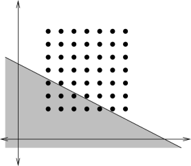
Figure 1: Visualization of two stock case

3.1 A Worst-Case or Best-Case Investor

Given a target return $\alpha$, this section focuses on how to compute an optimal portfolio for a worst-case risk-averse investor. The cases of a best-case risk-averse investor, a worst-case aggressive investor, and a best-case aggressive investor can be solved similarly.

We first present a basic algorithm to compute ${\cal RA_{\rm w}}(\alpha,\vec{x})$ by computing a worst-case joint distribution matrix $M$ for ${\cal S}_{1}$ and ${\cal S}_{2}$. For convenience, we index the entries of $M$ with $\{(i,j)\mid i,j=m_{1},\ldots,m_{2}\}$, where row $i$ (respectively, column $i$) corresponds to return $i\mu$ of $S_{1}$ (respectively, $j\mu$ of $S_{2}$). We model the problem of computing $M$ as a network flow problem on the graph $G$ defined below:

• $G$ has $2(m+1)$ vertices, namely, a source $s$, a sink $t$, and $v_{m_{1}},\ldots,v_{m_{2}}$, $w_{m_{1}},\ldots,w_{m_{2}}$, where $v_{i}$ (respectively, $w_{i}$) corresponds to return $i\mu$ of stock $S_{1}$ (respectively, stock $S_{2}$).

• For all $i,j=m_{1},\ldots,m_{2}$, $G$ has (1) edge $(v_{i},w_{j})$, which has capacity $c(v_{i},w_{j})=1$ if $x_{1}i\mu+x_{2}j\mu\leq\alpha$ or $0$ otherwise; (2) the edge $(s,v_{i})$ with capacity $c(s,v_{i})={\cal S}_{1}(i\mu)$; and (3) the edge $(w_{j},t)$ with capacity $c(w_{j},t)={\cal S}_{2}(j\mu)$.

Geometrically, we wish to push as much probability as possible into the region of $M$ defined by $x_{1}i+x_{2}j\leq\frac{\alpha}{\mu}$. In other words, the value of a maximum $s-t$ flow of $G$ equals ${\cal RA_{\rm w}}(\alpha,\vec{x})$. Thus, it is tempting to use a maximum flow algorithm to solve this maximum flow problem. The fastest known algorithm for this problem is due to Goldberg and Rao [Goldberg:1998:BFD] and runs in $O^{*}(m^{2\frac{2}{3}})$ time