Information Extraction
from Broadcast News

Abstract

This paper discusses the development of trainable statistical models for extracting content from television and radio news broadcasts. In particular we concentrate on statistical finite state models for identifying proper names and other named entities in broadcast speech. Two models are presented: the first represents name class information as a word attribute; the second represents both word-word and class-class transitions explicitly. A common $n$-gram based formulation is used for both models. The task of named entity identification is characterized by relatively sparse training data and issues related to smoothing are discussed. Experiments are reported using the DARPA/NIST Hub–4E evaluation for North American Broadcast News.

keywords: named entity; information extraction; language modelling

1 Introduction

Simple statistical models underlie many successful applications of speech and language processing. The most accurate document retrieval systems are based on unigram statistics. The acoustic model of virtually all speech recognition systems is based on stochastic finite state machines referred to as hidden Markov models (HMMs). The language (word sequence) model of state-of-the-art large vocabulary speech recognition systems uses an $n$-gram model ($[n-1]$th order Markov model), where $n$ is typically 4 or less. Two important features of these simple models are their trainability and scalability: in the case of language modelling, model parameters are frequently estimated from corpora containing up to $10^{9}$ words. These approaches have been extensively investigated and optimized for speech recognition, in particular, resulting in systems that can perform certain tasks (e.g., large vocabulary dictation from a cooperative speaker) with a high degree of accuracy. More recently, similar statistical finite state models have been developed for spoken language processing applications beyond direct transcription to enable, for example, the production of structured transcriptions which may include punctuation or content annotation.

In this paper we discuss the development of trainable statistical models for extracting content from television and radio news broadcasts. In particular, we concentrate on named entity (NE) identification, a task which is reviewed in §2. Section 3 outlines a general statistical framework for NE identification, based on an $n$-gram model over words and classes. We discuss two formulations of this basic approach. The first (§4) represents class information as a word attribute; the second (§5) explicitly represents word-word and class-class transitions. In both cases we discuss the implementation of the model and present results using an evaluation framework based on North American broadcast news data. Finally, in §6, we discuss our work in the context of other approaches to NE identification in spoken language and outline some areas for future work.

2 Named Entity Identification

2.1 Review

Proper names account for around 9% of broadcast news output, and their successful identification would be useful for structuring the output of a speech recognizer (through punctuation, capitalization and tokenization), and as an aid to other spoken language processing tasks, such as summarization and database creation. The task of NE identification involves identifying and classifying those words or word sequences that may be classified as proper names, or as certain other classes such as monetary expressions, dates and times. This is not a straightforward problem. While Wednesday 1 September is clearly a date, and Alan Turing is a personal name, other strings, such as the day after tomorrow, South Yorkshire Beekeepers Association and Nobel Prize are more ambiguous.

NE identification was formalized for evaluation purposes as part of the 5th Message Understanding Conference muc5:conf93, and the evaluation task definition has evolved since then. In this paper we follow the task definition specified for the recent broadcast news evaluation (referred to as Hub–4E IE–NE) sponsored by DARPA and NIST [Chinchor, Robinson, & BrownChinchor et al.1998]. This specification defined seven classes of named entity: three types of proper name ($\mathopen{<}$location$\mathclose{>}$, $\mathopen{<}$person$\mathclose{>}$ and $\mathopen{<}$organization$\mathclose{>}$) two types of temporal expression ($\mathopen{<}$date$\mathclose{>}$ and $\mathopen{<}$time$\mathclose{>}$) and two types of numerical expression ($\mathopen{<}$money$\mathclose{>}$ and $\mathopen{<}$percentage$\mathclose{>}$). According to this definition the following NE tags would be correct:

$\mathopen{<}$date$\mathclose{>}$Wednesday 1 September$\mathopen{<}$/date$\mathclose{>}$
$\mathopen{<}$person$\mathclose{>}$Alan Turing$\mathopen{<}$/person$\mathclose{>}$
the day after tomorrow
$\mathopen{<}$organization$\mathclose{>}$South Yorkshire Beekeepers Association$\mathopen{<}$/organization$\mathclose{>}$
Nobel Prize

The day after tomorrow is not tagged as a date, since only “absolute” time or date expressions are recognized; Nobel is not tagged as a personal name, since it is part of a larger construct that refers to the prize. Similarly, South Yorkshire is not tagged as a location since it is part of a larger construct tagged as an organization.

Both rule-based and statistical approaches have been used for NE identification. wakao:coling96 and hobbs:inbook97 adopted grammar-based approaches using specially constructed grammars, gazetteers of personal and company names, and higher level approaches such as name co-reference. Some grammar-based systems have utilized a trainable component, such as the Alembic system [Aberdeen, Burger, Day, Hirschman, Robinson, & VilainAberdeen et al.1995]. The LTG system [Mikheev, Grover, & MoensMikheev et al.1998] employed probabilistic partial matching, in addition to a non-probabilistic grammar and gazetteer look-up.

bikel:anlp97 introduced a purely trainable system for NE identification, which is discussed in greater detail in bikel:ml99. This approach was based on an ergodic HMM (i.e., an HMM in which every state is reachable from every state) where the hidden states corresponded to NE classes, and the observed symbols corresponded to words. Training was performed using an NE annotated corpus, so the state sequence was known at training time. Thus likelihood maximization could be accomplished directly without need for the expectation-maximization (EM) algorithm. The transition probabilities of this model were conditioned on both the previous state and the previous word, and the emission probabilities attached to each state could be regarded as a word-level bigram for the corresponding NE class.

NE identification systems are evaluated using an unseen set of evaluation data: the hypothesised NEs are compared with those annotated in a human-generated reference transcription. In this situation there are two possible types of error: type, where an item is tagged as the wrong kind of entity and extent, where the wrong number of word tokens are tagged. For example,

$\mathopen{<}$location$\mathclose{>}$South Yorkshire$\mathopen{<}$/location$\mathclose{>}$ Beekeepers Association

has errors of both type and extent since the ground truth for this excerpt is

$\mathopen{<}$organization$\mathclose{>}$South Yorkshire Beekeepers Association$\mathopen{<}$/organization$\mathclose{>}$ .

These two error types each contribute $0.5$ to the overall error count, and precision (P) and recall (R) can be calculated in the usual way. A weighted harmonic mean (P&R), sometimes called the F-measure [van Rijsbergenvan Rijsbergen1979], is often calculated as a single summary statistic:

$$P\&R=\frac{2RP}{R+P}\ .$$

In a recent evaluation, using newswire text, the best performing system mikheev:muc98 returned a P&R of 0.93. Although precision and recall are clearly informative measures, makhoul:darpa99 have criticized the use of P&R, since it implicitly deweights missing and spurious identification errors compared with incorrect identification errors. They proposed an alternative measure, referred to as the slot error rate (SER), that weights three types of identification error equally.

2.2 Identifying Named Entities in Speech

A straightforward approach to identifying named entities in speech is to transcribe the speech automatically using a recognizer, then to apply a text-based NE identification method to the transcription. It is more difficult to identify NEs from automatically transcribed speech compared with text, since speech recognition output is missing features that may be exploited by “hard-wired” grammar rules or by attachment to vocabulary items, such as punctuation, capitalization and numeric characters.

More importantly, no speech recognizer is perfect, and spoken language is rather different from written language. Although planned, low-noise speech (such as dictation, or a news bulletin read from a script) can be recognized with a word error rate (WER) of less than 10%, speech which is conversational, in a noisy (or otherwise cluttered) acoustic environment or from a different domain may suffer a WER in excess of 40%. Additionally, the natural unit seems to be the phrase, rather than the sentence, and phenomena such as disfluencies, corrections and repetitions are common. It could thus be argued that statistical approaches, that typically operate with limited context and very little notion of grammatical constructs, are more robust than grammar-based approaches. appelt:darpa99 oppose this argument, and have developed a finite-state grammar-based approach for NE identification of broadcast news. However, this relied on large, carefully constructed lexica and gazetteers, and it is not clear how portable between domains this approach is. Some further discussion of rule-based approaches follows in §6.

Spoken NE identification was first demonstrated by kubala:darpa98, who applied the model of bikel:ml99 to the output of a broadcast news speech recognizer. An important conclusion of that work — supported by the experiments reported here — was that the error of an NE identifier degraded linearly with WER, with the largest errors due to missing and spuriously tagged names. Since then several other researchers, including ourselves, have investigated the problem within the Hub–4E evaluation framework.

Evaluation of spoken NE identification is more complicated than for text, since there will be speech recognition errors as well as NE identification errors (i.e., the reference tags will not apply to the same word sequence as the hypothesised tags). This requires a word level alignment of the two word sequences, which may be achieved using a phonetic alignment algorithm developed for the evaluation of speech recognizers [Fisher & FiscusFisher and Fiscus1993]. Once an alignment is obtained, the evaluation procedure outlined above may be employed, with the addition of a third error type, content, caused by speech recognition errors. The same statistics (P&R and SER) can still be used, with the three error types contributing equally to the error count.

3 Statistical Framework

First, let ${\cal V}$ denote a vocabulary and ${\cal C}$ be a set of name classes. We consider that ${\cal V}$ is similar to a vocabulary for conventional speech recognition systems (i.e., typically containing tens of thousands of words, and no case information or other characteristics). In what follows, ${\cal C}$ contains the proper names, temporal and number expressions used in the Hub–4E IE–NE evaluation described above. When there is no ambiguity, these named entities are referred to as “name(s)”. As a convention here, a class $\mathopen{<}$other$\mathclose{>}$ is included in ${\cal C}$ for those words not belonging to any of the specified names. Because each name may consist of one word or a sequence of words, we also include a marker $\mathopen{<}$+$\mathclose{>}$ in ${\cal C}$, implying that the corresponding word is a part of the same name as the previous word. The following example is taken from a human-generated reference transcription for the 1997 Hub–4E Broadcast News evaluation data:

AT THE $\underbrace{\mbox{{\footnotesize RONALD REAGAN CENTER}}}_{\mbox{$\mathopen{<}${\footnotesize organization}$\mathclose{>}$}}$ IN $\underbrace{\mbox{{\footnotesize SIMI VALLEY}}}_{\mbox{$\mathopen{<}${\footnotesize location}$\mathclose{>}$}}$ $\underbrace{\mbox{{\footnotesize CALIFORNIA}}}_{\mbox{$\mathopen{<}${\footnotesize location}$\mathclose{>}$}}$

The corresponding class sequence is

$\mathopen{<}$other$\mathclose{>}$ $\mathopen{<}$+$\mathclose{>}$ $\mathopen{<}$organization$\mathclose{>}$ $\mathopen{<}$+$\mathclose{>}$ $\mathopen{<}$+$\mathclose{>}$ $\mathopen{<}$other$\mathclose{>}$ $\mathopen{<}$location$\mathclose{>}$ $\mathopen{<}$+$\mathclose{>}$ $\mathopen{<}$location$\mathclose{>}$

because SIMI VALLEY and CALIFORNIA are considered two different names by the specification chinchor:manual98b.

Figure 1: Topologies for NE models. The left model assumes that class information is a word attribute. The right model explicitly models word-word and class-class transitions.

Class information may be interpreted as a word attribute (the left model of figure 1). Formally, we define a class-word token $\mathop{\mathopen{<}c,w\mathclose{>}}\in{\cal C}\times{\cal V}$ and consider a probability

$${\textstyle p(\mathop{\mathopen{<}c,w\mathclose{>}}_{1},\cdots,\mathop{\mathopen{<}c,w\mathclose{>}}_{m})}=\prod_{i=1\cdots m}{\textstyle p(\mathop{\mathopen{<}c,w\mathclose{>}}_{i}|\mathop{\mathopen{<}c,w\mathclose{>}}_{1},\cdots,\mathop{\mathopen{<}c,w\mathclose{>}}_{i-1})}$$ (1)

that generates a sequence of class-word tokens $\mathop{\mathopen{<}c,w\mathclose{>}}_{1},\cdots,\mathop{\mathopen{<}c,w\mathclose{>}}_{m}$. Alternatively, word-word and class-class transitions may be explicitly formulated (the right model of figure 1). Then we consider a probability

$$p(c_{1},w_{1},\cdots,c_{m},w_{m})=\prod_{i=1\cdots m}p(c_{i},w_{i}|c_{1},w_{1},\cdots,c_{i-1},w_{i-1})$$ (2)

that generates a sequences of words $w_{1},\cdots,w_{m}$ and a corresponding sequence of classes $c_{1},\cdots,c_{m}$. The first approach is simple and analogous to conventional $n$-gram language modelling, however the performance is sub-optimal in comparison to the second approach, which is more complex and needs greater attention to the smoothing procedure.

For both formulations, we have performed experiments using data produced for the Hub–4E IE–NE evaluation. The training data for this evaluation consisted of manually annotated transcripts of the Hub–4E Broadcast News acoustic training data (broadcast in 1996–97). This data contained approximately one million words (corresponding to about 140 hours of audio). Development was performed using the 1997 evaluation data (3 hours of audio broadcast in 1996, about 32,000 words) and evaluation results reported on the 1998 evaluation data (3 hours of audio broadcast in 1996 and 1998, about 33,000 words).

4 Modelling Class Information as a Word Attribute

In this section, we describe an NE model based on direct word-word transitions, with class information treated as a word attribute. This approach suffers seriously from data sparsity. We briefly summarize why this is so.

4.1 Technical Description

Formulation (1) may be best viewed as a straightforward extension to standard $n$-gram language modelling. Denoting $e=\mathop{\mathopen{<}c,w\mathclose{>}}$, (1) is rewritten as

$${\textstyle p(e_{1},\cdots,e_{m})}=\prod_{i=1\cdots m}{\textstyle p(e_{i}|e_{1},\cdots,e_{i-1})}$$ (3)

and this is identical to the $n$-gram model widely used for large vocabulary speech recognition systems. Because each token $e\in{\cal C}\times{\cal V}$ is treated independently, those having the same word but the different class (e.g., $\mathopen{<}$date,MAY$\mathclose{>}$, $\mathopen{<}$person,MAY$\mathclose{>}$, and $\mathopen{<}$other,MAY$\mathclose{>}$) are considered different members. Using this formulation, class-class transitions are implicit. Further it may be interpreted as a classical HMM, in which tokens $e_{i}$ correspond to states, with observations $c_{i}$ and $w_{i}$ generated from each $e_{i}$. Maximum likelihood estimates for model parameters can be obtained from the frequency count of each $n$-gram given text data annotated with name information. Since the state sequence is known the forward-backward algorithm is not required. Standard discounting and smoothing techniques may be applied.

The search process is based on $n$-gram relations. Given a sequence of words, $w_{1},\cdots,w_{m}$, the most probable sequence of names may be identified by tracing the Viterbi path across the class-word trellis such that

$$\mathopen{<}\hat{c}_{1},\cdots,\hat{c}_{m}\mathclose{>}=\mathop{\rm argmax}_{c_{1}\cdots c_{m}}{\textstyle p(\mathop{\mathopen{<}c,w\mathclose{>}}_{1},\cdots,\mathop{\mathopen{<}c,w\mathclose{>}}_{m})}\ .$$ (4)

This process may be slightly elaborated by looking into a separate list of names that augments $n$-grams of $\mathop{\mathopen{<}c,w\mathclose{>}}$ tokens. Further technical details of this formulation are in gotoh:esca99.

4.2 Experiment

Using the experimental setup described in §3, we estimated a back-off trigram language model that contained $18,964$ class-word tokens in a trigram vocabulary, with a further $3,697$ words modelled as unigram extensions.

A hand transcription (provided by NIST) and four speech recognizer outputs (three distributed by NIST representing the range of systems that participated in the 1998 broadcast news transcription evaluation, and our own system [Robinson, Cook, Ellis, Fosler-Lussier, Renals, & WilliamsRobinson et al.]) were automatically marked with NEs, then scored against the human-generated reference transcription. The results are summarized in table 1. The combined P&R score was about 83% for a hand transcription. For recognizer outputs, the scores declined as WER increased. As noted by other researchers (e.g., miller:darpa99) a linear relationship between the WER and the NE identification scores is observed.

	WER	SER	R	P	P&R
hand transcription (NIST)	.000	.286	.799	.865	.831
recognizer output (NIST 1)	.135	.394	.738	.797	.766
(NIST 2)	.145	.399	.741	.791	.765
(NIST 3)	.283	.563	.618	.713	.662
recognizer output (own)	.210	.452	.700	.769	.733

Table 1: NE identification scores on 1998 Hub–4E evaluation data, using the NE model with implicit class transitions. A hand transcription and three recognizer outputs were provided by NIST. The bottom row is by our own recognizer. WER and SER indicate word and slot error rates. R, P, and P&R denote recall, precision, and a combined precision&recall scores, respectively. This table contains further improvement since our participation in the 1998 Hub–4E evaluation. In this experiment, we used transcripts of Broadcast News acoustic training data (1996–97) for NE model generation, but did not rely on external sources.

We have previously made an error analysis of this approach gotoh:esca99, where it was observed that most correctly marked names were identified through bigram or trigram constraints around each name (i.e., the name itself and words before/after that name). When the NE model was forced to back-off to unigram statistics, names were often missed (causing a decrease in recall) or occasionally a bigram of words attributed with another class was preferred (a decrease in precision). For example consider the phrase

… DIRECTOR ADRIAN LAJOUS SAYS …,

taken from the 1997 evaluation data, where LAJOUS was not found in the vocabulary. The maximum likelihood decoding for this phrase was:

… $\mathopen{<}$other,DIRECTOR$\mathclose{>}$ $\mathopen{<}$other,unknown$\mathclose{>}$ $\mathopen{<}$other,unknown$\mathclose{>}$ $\mathopen{<}$other,SAYS$\mathclose{>}$ …

Unigram statistics for $\mathopen{<}$person,ADRIAN$\mathclose{>}$ and $\mathopen{<}$person,unknown$\mathclose{>}$ existed in the model, however none of the trigrams or bigrams outperformed a bigram entry

$$p(\mbox{$\mathopen{<}${\footnotesize other,SAYS}$\mathclose{>}$}\ |\ \mbox{$\mathopen{<}${\footnotesize other,unknown}$\mathclose{>}$})\ .$$

Further, $\mathopen{<}$other,unknown$\mathclose{>}$ had higher unigram probability than $\mathopen{<}$person,ADRIAN$\mathclose{>}$, and no other trigram or bigram was able to recover this name. (There was no unigram entry for $\mathopen{<}$other,ADRIAN$\mathclose{>}$.) As a consequence, ADRIAN LAJOUS was not identified as $\mathopen{<}$person$\mathclose{>}$.

This is an example of a data sparsity problem that is observed in almost every aspect of spoken language processing. Although NE models cannot accommodate probability parameters for a complete set of $n$-gram occurrences, a successful recovery of name expressions is heavily dependent on the existence of higher order $n$-grams in the model. The implicit class transition approach contributes adversely to the data sparsity problem because it causes the set of possible tokens to increase in size from $|{\cal V}|$ to $|{\cal C}\times{\cal V}|$.

5 Explicit Modelling of Class and Word Transitions

In this section, an alternative formulation is presented that explicitly models constraints at the class level, compensating for the fundamental sparseness of $n$-gram tokens on a vocabulary set. Recent work by miller:darpa99 and palmer:darpa99 has indicated that such explicit modelling is a promising direction as $P\&R$ scores of up to 90% for hand transcribed data have been achieved using an ergodic HMM. These formulations may be regarded as a two-level architecture, in which the state transitions in the HMM represent transitions between classes (upper level), and the output distributions from each state correspond to the sequence of words within each class (lower level).

The formulation developed here is simpler because, rather than introducing a two-level architecture, we describe a flat state machine that models the probabilities of the current word and class conditioned on the previous word and class (the right model of figure 1). We do not describe this formulation as an HMM, as the probabilities are conditioned both on the previous word and on the previous class. Only a bigram model is considered; however it outperforms the trigram modelling of §4.

5.1 Technical Description

Formulation (2) treats class and word tokens independently. Using bigram level constraints, (2) is reduced to

$$p(c_{1},w_{1},\cdots,c_{m},w_{m})=\prod_{i=1\cdots m}p(c_{i},w_{i}|c_{i-1},w_{i-1})\ .$$ (5)

The right side of (5) may be decomposed as

$$p(c_{i},w_{i}|c_{i-1},w_{i-1})=p(w_{i}|c_{i},c_{i-1},w_{i-1})\cdot p(c_{i}|c_{i-1},w_{i-1})\ .$$ (6)

The conditioned current word probability $p(w_{i}|c_{i},c_{i-1},w_{i-1})$ and the current class probability $p(c_{i}|c_{i-1},w_{i-1})$ are in the same form as a conventional $n$-gram, hence may be estimated from annotated text data.

The amount of annotated text data available is orders of magnitude smaller than the amount of text data typically used to estimate $n$-gram language models for large vocabulary speech recognition. Smoothing the maximum likelihood probability estimates is therefore essential to avoid zero probabilities for events that were not observed in the training data. We have applied standard techniques in which more specific models are smoothed with progressively less specific models. The following smoothing path was chosen for the first term on the right side of (6):

$$p(w_{i}|c_{i},c_{i-1},w_{i-1})\longrightarrow p(w_{i}|c_{i},c_{i-1})\longrightarrow p(w_{i}|c_{i})\longrightarrow p(w_{i})\longrightarrow\frac{1}{|\cal W|}\ ,$$

where ${|\cal W|}$ is the size of the possible vocabulary that includes both observed and unobserved words from the training text data (i.e., ${|\cal W|}$ is sufficiently greater than $|{\cal V}|$). We preferred smoothing to $p(w_{i}|c_{i},c_{i-1})$, rather than to $p(w_{i}|c_{i},w_{i-1})$, since we believed that the former would be better estimated from the annotated training data.

Similarly, the smoothing path for the current class probability (the final term in (6)) was:

$$p(c_{i}|c_{i-1},w_{i-1})\longrightarrow p(c_{i}|c_{i-1})\longrightarrow p(c_{i})\ .$$

This assumes that each class occurs sufficiently in training text data; otherwise, further smoothing to some constant probability may be required.

Given the smoothing path, the current word probability may be computed using an interpolation method based on that of jelinek:proc80:

$$p(w_{i}|c_{i},c_{i-1},w_{i-1}) = \hat{f}(w_{i}|c_{i},c_{i-1},w_{i-1})$$ (7)

$$+\ \{1-\alpha(c_{i},c_{i-1},w_{i-1})\}\cdot p(w_{i}|c_{i},c_{i-1})$$

where $\hat{f}(w_{i}|c_{i},c_{i-1},w_{i-1})$ is a discounted relative frequency and $\alpha(c_{i},c_{i-1},w_{i-1})$ is a non-zero probability estimate (i.e., the probability that $\hat{f}(w_{i}|c_{i},c_{i-1},w_{i-1})$ exists in the model).

Alternatively, the back-off smoothing method of katz:assp87 could be applied:

$$p(w_{i}|c_{i},c_{i-1},w_{i-1})=\left\{\begin{array}[]{l}\hat{f}(w_{i}|c_{i},c_{i-1},w_{i-1})\qquad\,\mbox{if }{\cal E}(c_{i},w_{i}|c_{i-1},w_{i-1})\ \mbox{exists},\\ \beta(c_{i},c_{i-1},w_{i-1})\cdot p(w_{i}|c_{i},c_{i-1})\qquad\qquad\quad\mbox{otherwise}.\end{array}\right.$$ (10)

In (10), $\beta(c_{i},c_{i-1},w_{i-1})$ is a back-off factor and is calculated by

$$\beta(c_{i},c_{i-1},w_{i-1})=\displaystyle\frac{1-\alpha(c_{i},c_{i-1},w_{i-1})}{\displaystyle 1-\sum_{w_{i}\in{\cal E}(c_{i},w_{i}|c_{i-1},w_{i-1})}\hat{f}(w_{i}|c_{i},c_{i-1})}$$ (11)

where ${\cal E}(c_{i},w_{i}|c_{i-1},w_{i-1})$ implies the event such that current class $c_{i}$ and word $w_{i}$ occur after previous class $c_{i-1}$ and word $w_{i-1}$. Discounted relative frequencies and non-zero probability estimates may be obtained from training data using standard discounting techniques such as Good-Turing, absolute discounting, or deleted interpolation. Further discussion for discounting and smoothing approaches should be referred to, e.g., katz:assp87 or ney:pami95.

Given a sequence of words $w_{1},\cdots,w_{m}$, named entities can be identified by searching the Viterbi path such that

$$\mathopen{<}\hat{c}_{1}\cdots\hat{c}_{m}\mathclose{>}=\mathop{\rm argmax}_{c_{1}\cdots c_{m}}p(c_{1},w_{1},\cdots,c_{m},w_{m})\ .$$ (12)

Although the smoothing scheme should handle novel words well, the introduction of conditional probabilities for unknown (which represents those words not included in the vocabulary ${\cal V}$) may be used to model unknown words directly. In practice, this is achieved by setting a certain cutoff threshold when estimating discounting probabilities. Those words that occur less than this threshold are treated as unknown tokens. This does not imply that smoothing is no longer needed, but that conditional probabilities containing the unknown token may occasionally pick up the context correctly without smoothing with weaker models. The drawback is that some uncommon words are lost from the vocabulary. Below we compare two NE models experimentally: one with unknown and fewer vocabulary words and the other without unknown but with more vocabulary words.

5.2 Experiment

Experiments were performed using the evaluation conditions described in §3. Two NE models (with explicit class transitions) were derived from transcripts of the hand annotated Broadcast News acoustic training data. One model contained no unknown token; there existed 27,280 different words in the training data, all of which were accommodated in the vocabulary list. Another model selected 17,560 words (from those occurring more than once in the training data) as a vocabulary and the rest (those occurring exactly once — nearly 10,000 words) were replaced by the unknown token.

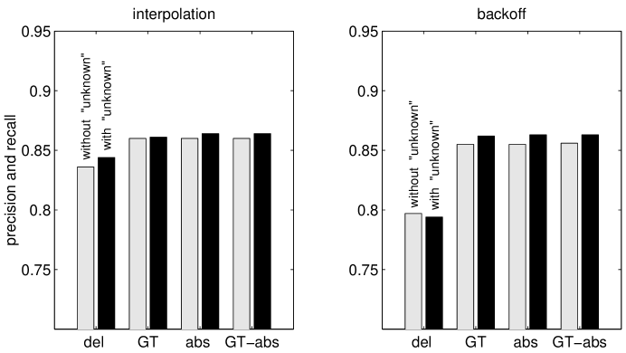
Figure 2: NE identification scores (P&R) on 1997 Hub–4E hand transcription — calculated using interpolation and back-off smoothing. NE models were built with and without the unknown token, using deleted interpolation (del), Good-Turing (GT), absolute (abs), and a combination of Good-Turing/absolute (GT-abs) discounting schemes. We have used 1997 data for a system development (as in figure 2), then applied to 1998 data for a system evaluation (as in table 2).

Firstly, NE models were discounted using the deleted interpolation, absolute, Good-Turing and combined Good-Turing/absolute discounting schemes. For each discounting scheme and with/without an unknown token, figure 2 shows P&R scores using the hand transcription of the 1997 evaluation data. For most cases, P&R was slightly better when unknown was introduced, although the vocabulary size was substantially smaller. Among discounting schemes, there was hardly any difference between Good-Turing, absolute, and combined Good-Turing/absolute, regardless of the smoothing method used. Non-zero probability parameters derived using deleted interpolation did not seem well matched to back-off smoothing. We suspect, however, that the difference in performance would be negligible if a sufficient amount of training data was available for the deleted interpolation case.

Using unknown and the combined Good-Turing/absolute discounting scheme, followed by back-off smoothing, table 2 summarizes NE identification scores for 1998 Hub–4E evaluation data. For the hand transcription and the four speech recognition outputs, this explicit class transition NE model improved P&R scores by 4–6% absolute over the implicit model of §4.

	WER	SER	R	P	P&R
hand transcription (NIST)	.000	.187	.863	.922	.892
recognizer output (NIST 1)	.135	.305	.775	.860	.815
(NIST 2)	.145	.296	.779	.867	.821
(NIST 3)	.283	.469	.655	.783	.713
recognizer output (own)	.210	.381	.729	.823	.773

Table 2: NE identification scores on 1998 Hub–4E evaluation data, using the NE model with explicit class transitions. A hand transcription and three recognizer outputs were provided by NIST. The bottom row is by our own recognizer. WER and SER indicate word and slot error rates. R, P, and P&R denote recall, precision, and a combined precision&recall scores, respectively. The NE model contained 17,560 vocabulary words plus unknown token. A combination of Good-Turing/absolute discounting scheme was applied, followed by back-off smoothing. The best performing model in the 1998 Hub–4E IE–NE miller:darpa99 had P&R scores of .906, .815, .826, and .703 for the hand transcription and NIST recognizer outputs 1, 2, 3.

Although more complex in formulation, it is beneficial to model class-class transitions explicitly. Consider again the phrase … DIRECTOR ADRIAN LAJOUS SAYS … discussed in §4. Here, ADRIAN LAJOUS was correctly identified as $\mathopen{<}$person$\mathclose{>}$ although LAJOUS was not included in the vocabulary. It was identified using the product of conditional probabilities

$$p(\mbox{{\small unknown}}\ |\ \mbox{$\mathopen{<}${\footnotesize+}$\mathclose{>}$},\mbox{$\mathopen{<}${\footnotesize person}$\mathclose{>}$})\cdot p(\mbox{$\mathopen{<}${\footnotesize+}$\mathclose{>}$}\ |\ \mbox{$\mathopen{<}${\footnotesize person}$\mathclose{>}$},\mbox{{\footnotesize ADRIAN}})$$

between ADRIAN and unknown  as well as the product

$$p(\mbox{{\footnotesize SAYS}}\ |\ \mbox{$\mathopen{<}${\footnotesize other}$\mathclose{>}$},\mbox{$\mathopen{<}${\footnotesize person}$\mathclose{>}$},\mbox{{\small unknown}})\cdot p(\mbox{$\mathopen{<}${\footnotesize other}$\mathclose{>}$}\ |\ \mbox{$\mathopen{<}${\footnotesize person}$\mathclose{>}$},\mbox{{\small unknown}})$$

between unknown and SAYS.

5.3 An Alternative Decomposition

There exists an alternative approach to decomposing the right side of Equation (5):

$$p(c_{i},w_{i}|c_{i-1},w_{i-1})=p(c_{i}|w_{i},c_{i-1},w_{i-1})\cdot p(w_{i}|c_{i-1},w_{i-1})\ .$$ (13)

Theoretically, if the “true” conditional probability can be estimated, decompositions by (6) and by (13) should produce identical results. This ideal case does not occur, and various discounting and smoothing techniques will cause further differences between two decompositions.

In practice, the conditional probabilities on the right side of (13) can be estimated in the same fashion as described in §4: counting the occurrences of each token in annotated text data, then applying certain discounting and smoothing techniques. The adopted smoothing path for the current word probability was

$$p(w_{i}|c_{i-1},w_{i-1})\longrightarrow p(w_{i}|c_{i-1})\longrightarrow p(w_{i})\longrightarrow\frac{1}{|\cal W|}$$

and a path for the current class probability was

$$p(c_{i}|w_{i},c_{i-1})\longrightarrow p(c_{i}|w_{i})\longrightarrow p(c_{i})\ .$$

In the latter case, a slight approximation $p(c_{i}|w_{i},c_{i-1},w_{i-1})\sim p(c_{i}|w_{i},c_{i-1})$ was made, since it was observed that $w_{i-1}$ did not contribute much when calculating the probability of $c_{i}$ in this manner.

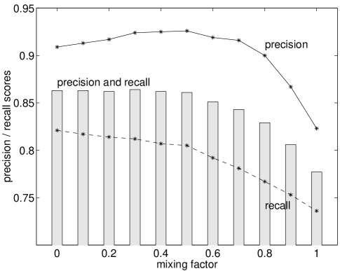
Figure 3: P&R scores on the 1997 hand transcription using mixtures of the two decompositions. NE models were built using unknown  combined Good-Turing/absolute discounting, then back-off smoothing.

This second decomposition alone did not work as well as the initial decomposition. When applied to the 1997 hand transcription, the P&R score declined by 8% absolute (using unknown, combined Good-Turing/absolute discounting, and back-off smoothing). In general, decomposition by (13) accurately tagged words that occurred frequently in the training data, but performed less well for uncommon words. Crudely speaking, it calculated the distribution over classes for each word; consequently it had reduced accuracy for uncommon words with less reliable probability estimates. Decomposition by (6) makes a more balanced decision because it relies on the distribution over words for each class, and there are orders of magnitude fewer classes than words.

The two decompositions can be combined by

$$p(c_{i},w_{i}|c_{i-1},w_{i-1})=p_{1}(c_{i},w_{i}|c_{i-1},w_{i-1})^{1-k}\cdot p_{2}(c_{i},w_{i}|c_{i-1},w_{i-1})^{k}$$ (14)

where $p_{1}$ refers to the initial method and $p_{2}$ the alternative. Figure 3 shows precision and recall scores for the mixture (with factors $0.0\leq k\leq 1.0$) of the two decompositions. It is observed that, for values of $k$ around $0.5$, this modelling improved the precision without degrading the overall P&R.

6 Discussion

We have described trainable statistical models for the identification of named entities in television and radio news broadcasts. Two models were presented, both based on $n$-gram statistics. The first model — in which class information was implicitly modelled as a word attribute — was a straightforward extension of conventional language modelling. However, it suffered seriously from the problem of data sparsity, resulting in a sub-optimal performance (a P&R score of 83% on a hand transcription). We addressed this problem in a second approach which explicitly modelled class-class and word-word transitions. With this approach the P&R score improved to 89%. These scores were based on a relatively small amount of training data (one million words). Like other language modelling problems, a simple way to improve the performance is to increase the amount of training data. miller:darpa99 have noted that there is a log-linear relation between the amount of training data and the NE identification performance; our experiments indicate that the P&R score improves by a few percent for each doubling of the training data size (between 0.1 and 1.0 million words).

The development of the second model was motivated by the success of the approach of bikel:ml99 and miller:darpa99. This model shares the same principle of an explicit, statistical model of class-class and word-word transitions, but the model formulation, and the discounting and smoothing procedures differ. In particular, the model presented here is a flat state machine, that is not readily interpretable as a two-level HMM architecture. Our experience indicates that an appropriate choice and implementation of discounting/smoothing strategies is very important, since a more complex model structure is being trained with less data, compared with conventional language models for speech recognition systems. The overall results that we have obtained are similar to those of miller:darpa99, but there are some differences which we cannot immediately explain away. In particular, although the combined P&R scores were similar, miller:darpa99 reported balanced recall and precision, whereas we have consistently observed substantially higher precision and lower recall.

The models presented here were trained using a corpus of about one million words of text, manually annotated. No gazetteers, carefully-tuned lexica or domain-specific rules were employed; the brittleness of maximum likelihood estimation procedures when faced with sparse training data was alleviated by automatic smoothing procedures. Although the fact that an accurate NE model can be estimated from sparse training data is of considerable interest and import, it is clear that it would be of use to be able to incorporate much more information in a statistical NE identifier. To this end, we are investigating two basic approaches: the incorporation of prior information; and unsupervised learning.

The most developed uses of prior information for NE identification are in the form of the rule-based systems developed for the task. Some initial work, carried out with Rob Gaizauskas and Mark Stevenson using a development of the system described by wakao:coling96, has analysed the errors of rule-based and statistical approaches. This has indicated that there is a significant difference between the annotations produced by the two systems for the three classes of proper name. This leads us to believe that there is some scope for either merging the outputs of the two systems, or incorporating some aspects of the rule-based systems as prior knowledge in the statistical system.

Unsupervised learning of statistical NE models is attractive, since manual NE annotation of transcriptions is a labour intensive process. However, our preliminary experiments indicate that unsupervised training of NE models is not straightforward. Using a model built from 0.1 million words of manually annotated text, the rest of the training data was automatically annotated, and the process iterated. P&R scores stayed at the same level (around 73%) regardless of iteration.

Finally, we note that the NE annotation models discussed here — and all other state-of-the-art approaches — act as a post-processor to a speech recognizer. Hence the strong correlation between the P&R scores of the NE tagger and the WER of the underlying speech recognizer is to be expected. The development of NE models that incorporate acoustic information such as prosody [Hakkani Tür, Tür, Stolcke, & ShribergHakkani Tür et al.1999] and confidence measures [Palmer, Ostendorf, & BurgerPalmer et al.1999] are future directions of interest.

Acknowledgements.

We have benefited greatly from cooperation and discussions with Robert Gaizauskas and Mark Stevenson. We thank BBN and MITRE for the provision of manually-annotated training data. The evaluation infrastructure was provided by MITRE, NIST and SAIC. This work was supported by EPSRC grant GR/M36717.

References

- [\citeauthoryearAberdeen, Burger, Day, Hirschman, Robinson, & VilainAberdeen et al.1995] Aberdeen, J., Burger, J., Day, D., Hirschman, L., Robinson, P., & Vilain, M. (1995). MITRE: Description of the Alembic system used for MUC-6. In Proceedings of the 6th Message Understanding Conference (MUC-6), Maryland, pp. 141–155.
- [\citeauthoryearAppelt & MartinAppelt and Martin1999] Appelt, D. E. & Martin, D. (1999). Named entity extraction from speech: Approach and results using the TextPro system. In Proceedings of DARPA Broadcast News Workshop, Herndon, VA, pp. 51–54.
- [\citeauthoryearBikel, Miller, Schwartz, & WeischedelBikel et al.1997] Bikel, D. M., Miller, S., Schwartz, R., & Weischedel, R. (1997). Nymble: a high-performance learning name-finder. In Proceedings of the 5th ANLP, Washington, DC, pp. 194–201.
- [\citeauthoryearBikel, Schwartz, & WeischedelBikel et al.1999] Bikel, D. M., Schwartz, R., & Weischedel, R. M. (1999). An algorithm that learns what’s in a name. Machine Learning 34, 211–231.
- [\citeauthoryearChinchor, Robinson, & BrownChinchor et al.1998] Chinchor, N., Robinson, P., & Brown, E. (1998). Hub-4 Named Entity Task Definition (version 4.8). SAIC. (http://www.nist.gov/speech/hub4_98/hub4_98.htm).
- [\citeauthoryearFisher & FiscusFisher and Fiscus1993] Fisher, W. & Fiscus, J. (1993). Better alignment procedures for speech recognition evaluation. In Proceedings of ICASSP-93, Volume 2, Minneapolis, pp. 59–62.
- [\citeauthoryearGotoh & RenalsGotoh and Renals1999] Gotoh, Y. & Renals, S. (1999). Statistical annotation of named entities in spoken audio. In Proceedings of the ESCA Workshop: Accessing Information in Spoken Audio, Cambridge, pp. 43–48. (http://svr-www.eng.cam.ac.uk/~ajr/esca99/).
- [\citeauthoryearHakkani Tür, Tür, Stolcke, & ShribergHakkani Tür et al.1999] Hakkani Tür, D., Tür, G., Stolcke, A., & Shriberg, E. (1999). Combining words and prosody for information extraction from speech. In Proceedings of Eurospeech-99, Volume 5, Budapest, pp. 1991–1994.
- [\citeauthoryearHobbs, Appelt, Bear, Israel, Kameyama, Stickel, & TysonHobbs et al.1997] Hobbs, J., Appelt, D., Bear, J., Israel, D., Kameyama, M., Stickel, M., & Tyson, M. (1997). FASTUS: A cascaded finite state transducer for extracting information from natural language text. In E. Roche & Y. Schabes (Eds.), Finite State Language Processing, pp. 381–406. MIT Press.
- [\citeauthoryearJelinek & MercerJelinek and Mercer1980] Jelinek, F. & Mercer, R. L. (1980). Interpolated estimation of Markov source parameters from sparse data. In Proceedings of the Workshop: Pattern Recognition in Practice, Amsterdam, pp. 381–397.
- [\citeauthoryearKatzKatz1987] Katz, S. M. (1987). Estimation of probabilities from sparse data for the language model component of a speech recognizer. IEEE Transactions on Acoustics, Speech, and Signal Processing 35(3), 400–401.
- [\citeauthoryearKubala, Schwartz, Stone, & WeischedelKubala et al.1998] Kubala, F., Schwartz, R., Stone, R., & Weischedel, R. (1998). Named entity extraction from speech. In Proceedings of DARPA Broadcast News Transcription and Understanding Workshop, Lansdowne, VA.
- [\citeauthoryearMakhoul, Kubala, Schwartz, & WeischedelMakhoul et al.1999] Makhoul, J., Kubala, F., Schwartz, R., & Weischedel, R. (1999). Performance measures for information extraction. In Proceedings of DARPA Broadcast News Workshop, Herndon, VA, pp. 249–252.
- [\citeauthoryearMikheev, Grover, & MoensMikheev et al.1998] Mikheev, A., Grover, C., & Moens, M. (1998). Description of the LTG system used for MUC-7. In Proceedings of the 7th Message Understanding Conference (MUC-7).
- [\citeauthoryearMiller, Schwartz, Weischedel, & StoneMiller et al.1999] Miller, D., Schwartz, R., Weischedel, R., & Stone, R. (1999). Named entity extraction from broadcast news. In Proceedings of DARPA Broadcast News Workshop, Herndon, VA, pp. 37–40.
- [\citeauthoryearMUC-5MUC-51993] MUC-5 (1993). Proceedings of the fifth message understanding conference.
- [\citeauthoryearNey, Essen, & KneserNey et al.1995] Ney, H., Essen, U., & Kneser, R. (1995). On the estimation of ‘small’ probabilities by leaving-one-out. IEEE Transactions on Pattern Analysis and Machine Intelligence 17(12), 1202–1212.
- [\citeauthoryearPalmer, Burger, & OstendorfPalmer et al.1999] Palmer, D. D., Burger, J. D., & Ostendorf, M. (1999). Information extraction from broadcast news speech data. In Proceedings of DARPA Broadcast News Workshop, Herndon, VA, pp. 41–46.
- [\citeauthoryearPalmer, Ostendorf, & BurgerPalmer et al.1999] Palmer, D. D., Ostendorf, M., & Burger, J. D. (1999). Robust information extraction from spoken language data. In Proceedings of Eurospeech-99, Volume 3, Budapest, pp. 1035–1038.
- [\citeauthoryearRobinson, Cook, Ellis, Fosler-Lussier, Renals, & WilliamsRobinson et al.] Robinson, A. J., Cook, G. D., Ellis, D. P. W., Fosler-Lussier, E., Renals, S. J., & Williams, D. A. G. Connectionist speech recognition of broadcast news. Submitted to Speech Communication.
- [\citeauthoryearRobinson, Brown, Burger, Chinchor, Douthat, Ferro, & HirschmanRobinson et al.1999] Robinson, P., Brown, E., Burger, J., Chinchor, N., Douthat, A., Ferro, L., & Hirschman, L. (1999). Overview: Information extraction from broadcast news. In Proceedings of DARPA Broadcast News Workshop, Herndon, VA, pp. 27–30.
- [\citeauthoryearvan Rijsbergenvan Rijsbergen1979] van Rijsbergen, C. J. (1979). Information Retrieval (2nd ed.). London: Butterworths.
- [\citeauthoryearWakao, Gaizauskas, & WilksWakao et al.1996] Wakao, T., Gaizauskas, R., & Wilks, Y. (1996). Evaluation of an algorithm for the recognition and classification of proper names. In Proceedings of COLING-96, Copenhagen, pp. 418–423.