Advances in domain independent linear text segmentation

Abstract

This paper describes a method for linear text segmentation which is twice as accurate and over seven times as fast as the state-of-the-art [Reynar, 1998]. Inter-sentence similarity is replaced by rank in the local context. Boundary locations are discovered by divisive clustering.

1 Introduction

Even moderately long documents typically address several topics or different aspects of the same topic. The aim of linear text segmentation is to discover the topic boundaries. The uses of this procedure include information retrieval [Hearst and Plaunt, 1993, Hearst, 1994, Yaari, 1997, Reynar, 1999], summarization [Reynar, 1998], text understanding, anaphora resolution [Kozima, 1993], language modelling [Morris and Hirst, 1991, Beeferman et al., 1997b] and improving document navigation for the visually disabled [Choi, 2000].

This paper focuses on domain independent methods for segmenting written text. We present a new algorithm that builds on previous work by Reynar [Reynar, 1998, Reynar, 1994]. The primary distinction of our method is the use of a ranking scheme and the cosine similarity measure [van Rijsbergen, 1979] in formulating the similarity matrix. We propose that the similarity values of short text segments is statistically insignificant. Thus, one can only rely on their order, or rank, for clustering.

2 Background

Existing work falls into one of two categories, lexical cohesion methods and multi-source methods [Yaari, 1997]. The former stem from the work of Halliday and Hasan [Halliday and Hasan, 1976]. They proposed that text segments with similar vocabulary are likely to be part of a coherent topic segment. Implementations of this idea use word stem repetition [Youmans, 1991, Reynar, 1994, Ponte and Croft, 1997], context vectors [Hearst, 1994, Yaari, 1997, Kaufmann, 1999, Eichmann et al., 1999], entity repetition [Kan et al., 1998], semantic similarity [Morris and Hirst, 1991, Kozima, 1993], word distance model [Beeferman et al., 1997a] and word frequency model [Reynar, 1999] to detect cohesion. Methods for finding the topic boundaries include sliding window [Hearst, 1994], lexical chains [Morris, 1988, Kan et al., 1998], dynamic programming [Ponte and Croft, 1997, Heinonen, 1998], agglomerative clustering [Yaari, 1997] and divisive clustering [Reynar, 1994]. Lexical cohesion methods are typically used for segmenting written text in a collection to improve information retrieval [Hearst, 1994, Reynar, 1998].

Multi-source methods combine lexical cohesion with other indicators of topic shift such as cue phrases, prosodic features, reference, syntax and lexical attraction [Beeferman et al., 1997a] using decision trees [Miike et al., 1994, Kurohashi and Nagao, 1994, Litman and Passonneau, 1995] and probabilistic models [Beeferman et al., 1997b, Hajime et al., 1998, Reynar, 1998]. Work in this area is largely motivated by the topic detection and tracking (TDT) initiative [Allan et al., 1998]. The focus is on the segmentation of transcribed spoken text and broadcast news stories where the presentation format and regular cues can be exploited to improve accuracy.

3 Algorithm

Our segmentation algorithm takes a list of tokenized sentences as input. A tokenizer [Grefenstette and Tapanainen, 1994] and a sentence boundary disambiguation algorithm [Palmer and Hearst, 1994, Reynar and Ratnaparkhi, 1997] or EAGLE [Reynar et al., 1997] may be used to convert a plain text document into the acceptable input format.

3.1 Similarity measure

Punctuation and uninformative words are removed from each sentence using a simple regular expression pattern matcher and a stopword list. A stemming algorithm [Porter, 1980] is then applied to the remaining tokens to obtain the word stems. A dictionary of word stem frequencies is constructed for each sentence. This is represented as a vector of frequency counts.

Let $f_{i,j}$ denote the frequency of word $j$ in sentence $i$. The similarity between a pair of sentences $x,y$ is computed using the cosine measure as shown in equation 1. This is applied to all sentence pairs to generate a similarity matrix.

$$sim(x,y)=\frac{\sum_{j}f_{x,j}\times f_{y,j}}{\sqrt{{\sum_{j}f_{x,j}^{2}}\times{\sum_{j}f_{y,j}^{2}}}}$$ (1)

Figure 1 shows an example of a similarity matrix. High similarity values are represented by bright pixels. The bottom-left and top-right pixel show the self-similarity for the first and last sentence, respectively. Notice the matrix is symmetric and contains bright square regions along the diagonal. These regions represent cohesive text segments.

Figure 1: An example similarity matrix.

3.2 Ranking

For short text segments, the absolute value of $sim(x,y)$ is unreliable. An additional occurrence of a common word (reflected in the numerator) causes a disproportionate increase in $sim(x,y)$ unless the denominator (related to segment length) is large. Thus, in the context of text segmentation where a segment has typically $<100$ informative tokens, one can only use the metric to estimate the order of similarity between sentences, e.g. $a$ is more similar to $b$ than $c$.

Furthermore, language usage varies throughout a document. For instance, the introduction section of a document is less cohesive than a section which is about a particular topic. Consequently, it is inappropriate to directly compare the similarity values from different regions of the similarity matrix.

In non-parametric statistical analysis, one compares the rank of data sets when the qualitative behaviour is similar but the absolute quantities are unreliable. We present a ranking scheme which is an adaptation of that described in [O’Neil and Denos, 1992].

Each value in the similarity matrix is replaced by its rank in the local region. The rank is the number of neighbouring elements with a lower similarity value. Figure 2 shows an example of image ranking using a $3\times 3$ rank mask with output range $\{0,8\}$. For segmentation, we used a $11\times 11$ rank mask. The output is expressed as a ratio $r$ (equation 2) to circumvent normalisation problems (consider the cases when the rank mask is not contained in the image).

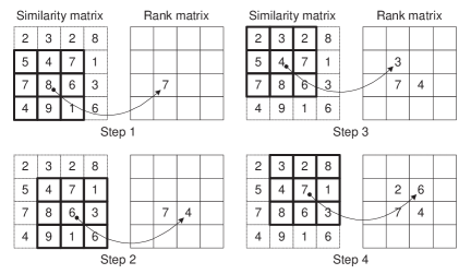
Figure 2: A working example of image ranking.

$$r=\frac{\textrm{\# of elements with a lower value}}{\textrm{\# of elements examined}}$$ (2)

To demonstrate the effect of image ranking, the process was applied to the matrix shown in figure 1 to produce figure 3. Notice the contrast has been improved significantly. Figure 4 illustrates the more subtle effects of our ranking scheme. $r(x)$ is the rank ($1\times 11$ mask) of $f(x)$ which is a sine wave with decaying mean, amplitude and frequency (equation 3).

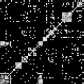
Figure 3: The matrix in figure 1 after ranking.

$$\begin{array}[]{rcl}f(x)&=&g(x\times\frac{2\pi}{200})\\ &&\\ g(z)&=&\frac{1}{2}(e^{-z/2}+\frac{1}{2}e^{-z/2}(1+\sin(10z^{0.7})))\\ \end{array}$$ (3)

Figure 4: An illustration of the more subtle effects of our ranking scheme.

3.3 Clustering

The final process determines the location of the topic boundaries. The method is based on Reynar’s maximisation algorithm [Reynar, 1998, Helfman, 1996, Church, 1993, Church and Helfman, 1993]. A text segment is defined by two sentences $i,j$ (inclusive). This is represented as a square region along the diagonal of the rank matrix. Let $s_{i,j}$ denote the sum of the rank values in a segment and $a_{i,j}=(j-i+1)^{2}$ be the inside area. $B=\{b_{1},...,b_{m}\}$ is a list of $m$ coherent text segments. $s_{k}$ and $a_{k}$ refers to the sum of rank and area of segment $k$ in $B$. $D$ is the inside density of $B$ (see equation 4).

$$D=\frac{\sum_{k=1}^{m}s_{k}}{\sum_{k=1}^{m}a_{k}}$$ (4)

To initialise the process, the entire document is placed in $B$ as one coherent text segment. Each step of the process splits one of the segments in $B$. The split point is a potential boundary which maximises $D$. Figure 5 shows a working example.

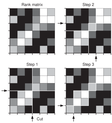
Figure 5: A working example of the divisive clustering algorithm.

The number of segments to generate, $m$, is determined automatically. $D^{(n)}$ is the inside density of $n$ segments and $\delta D^{(n)}=D^{(n)}-D^{(n-1)}$ is the gradient. For a document with $b$ potential boundaries, $b$ steps of divisive clustering generates $\{D^{(1)},...,D^{(b+1)}\}$ and $\{\delta D^{(2)},...,\delta D^{(b+1)}\}$ (see figure 6 and 7). An unusually large reduction in $\delta D$ suggests the optimal clustering has been obtained (see $n=10$ in figure 7). Let $\mu$ and $\nu$ be the mean and variance of $\delta D^{(n)},n\in\{2,...,b+1\}$. $m$ is obtained by applying the threshold, $\mu+c\times\sqrt{\nu}$, to $\delta D$ ($c=1.2$ works well in practice).

Figure 6: The inside density of all levels of segmentation.

Figure 7: Finding the optimal segmentation using the gradient.

3.4 Speed optimisation

The running time of each step is dominated by the computation of $s_{k}$. Given $s_{i,j}$ is constant, our algorithm pre-computes all the values to improve speed performance. The procedure computes the values along diagonals, starting from the main diagonal and works towards the corner. The method has a complexity of order $1\frac{1}{2}n^{2}$. Let $r_{i,j}$ refer to the rank value in the rank matrix $R$ and $S$ to the sum of rank matrix. Given $R$ of size $n\times n$, $S$ is computed in three steps (see equation 5). Figure 8 shows the result of applying this procedure to the rank matrix in figure 5.

$$\begin{array}[]{llcl}1.&s_{i,i}&=&r_{i,i}\\ &&\textrm{for}&i\in\{1,...,n\}\\ 2.&s_{i+1,i}&=&2r_{i+1,i}+s_{i,i}+s_{i+1,i+1}\\ &s_{i,i+1}&=&s_{i+1,i}\\ &&\textrm{for}&i\in\{1,...,n-1\}\\ 3.&s_{i+j,i}&=&2r_{i+j,i}+s_{i+j-1,i}+\\ &&&s_{i+j,i+1}-s_{i+j-1,i+1}\\ &s_{i,i+j}&=&s_{i+j,i}\\ &&\textrm{for}&j\in\{2,...,n-1\}\\ &&&i\in\{1,...,n-j\}\\ \end{array}$$ (5)

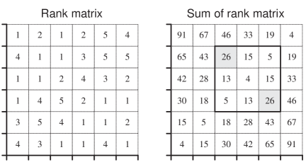
Figure 8: Improving speed performance by pre-computing $s_{i,j}$.

4 Evaluation

The definition of a topic segment ranges from complete stories [Allan et al., 1998] to summaries [Ponte and Croft, 1997]. Given the quality of an algorithm is task dependent, the following experiments focus on the relative performance. Our evaluation strategy is a variant of that described in [Reynar, 1998, 71-73] and the TDT segmentation task [Allan et al., 1998]. We assume a good algorithm is one that finds the most prominent topic boundaries.

4.1 Experiment procedure

An artificial test corpus of 700 samples is used to assess the accuracy and speed performance of segmentation algorithms. A sample is a concatenation of ten text segments. A segment is the first $n$ sentences of a randomly selected document from the Brown corpus. A sample is characterised by the range of $n$. The corpus was generated by an automatic procedure. Table 1 presents the corpus statistics.

Range of $n$	$3-11$	$3-5$	$6-8$	$9-11$
# samples	400	100	100	100

Table 1: Test corpus statistics.

$$\begin{array}[]{l}p(\textrm{error}|\textrm{ref},\textrm{hyp},k)=\\ \quad p(\textrm{miss}|\textrm{ref},\textrm{hyp},\textrm{diff},k)p(\textrm{diff}|\textrm{ref},k)+\\ \quad p(\textrm{fa}|\textrm{ref},\textrm{hyp},\textrm{same},k)p(\textrm{same}|\textrm{ref},k)\\ \end{array}$$ (6)

Speed performance is measured by the average number of CPU seconds required to process a test sample. Segmentation accuracy is measured by the error metric (equation 6, fa $\to$ false alarms) proposed in [Beeferman et al., 1999]. Low error probability indicates high accuracy. Other performance measures include the popular precision and recall metric (PR) [Hearst, 1994], fuzzy PR [Reynar, 1998] and edit distance [Ponte and Croft, 1997]. The problems associated with these metrics are discussed in [Beeferman et al., 1999].

4.2 Experiment 1 - Baseline

Five degenerate algorithms define the baseline for the experiments. $B_{n}$ does not propose any boundaries. $B_{a}$ reports all potential boundaries as real boundaries. $B_{e}$ partitions the sample into regular segments. $B_{(r,?)}$ randomly selects any number of boundaries as real boundaries. $B_{(r,b)}$ randomly selects $b$ boundaries as real boundaries.

The accuracy of the last two algorithms are computed analytically. We consider the status of $m$ potential boundaries as a bit string ($1\to$ topic boundary). The terms $p(\textrm{miss})$ and $p(\textrm{fa})$ in equation 6 corresponds to $p(\textrm{same}|k)$ and $p(\textrm{diff}|k)=1-p(\textrm{same}|k)$. Equation 7, 8 and 9 gives the general form of $p(\textrm{same}|k)$, $B_{(r,?)}$ and $B_{(r,b)}$, respectively.

Table 2 presents the experimental results. The values in row two and three, four and five are not actually the same. However, their differences are insignificant according to the Kolmogorov-Smirnov, or KS-test [Press et al., 1992].

$$p(\textrm{same}|k)=\frac{\textrm{\# valid segmentations}}{\textrm{\# possible segmentations}}$$ (7)

$$p(\textrm{same}|k,B_{(r,?)})=\frac{2^{m-k}}{2^{m}}=2^{-k}$$ (8)

$$\begin{array}[]{rcl}p(\textrm{same}|k,m,B_{(r,b)})&=&\frac{{}_{(m-k)}C_{b}}{{}_{m}C_{b}}\\ &&\\ {}_{x}C_{y}&=&\frac{x!}{y!(x-y)!}\\ \end{array}$$ (9)

	3-11	3-5	6-8	9-11
$B_{e}$	45%	38%	39%	36%
$B_{n}$	47%	47%	47%	46%
$B_{(r,b)}$	47%	47%	47%	46%
$B_{a}$	53%	53%	53%	54%
$B_{(r,?)}$	53%	53%	53%	54%

Table 2: The error rate of the baseline algorithms.

4.3 Experiment 2 - TextTiling

We compare three versions of the TextTiling algorithm [Hearst, 1994]. $H94_{(c,d)}$ is Hearst’s C implementation with default parameters. $H94_{(c,r)}$ uses the recommended parameters $k=6$, $w=20$. $H94_{(j,r)}$ is my implementation of the algorithm. Experimental result (table 3) shows $H94_{(c,d)}$ and $H94_{(c,r)}$ are more accurate than $H94_{(j,r)}$. We suspect this is due to the use of a different stopword list and stemming algorithm.

	3-11	3-5	6-8	9-11
$H94_{(c,d)}$	46%	44%	43%	48%
$H94_{(c,r)}$	46%	44%	44%	49%
$H94_{(j,r)}$	54%	45%	52%	53%
$H94_{(c,d)}$	0.67s	0.52s	0.66s	0.88s
$H94_{(c,r)}$	0.68s	0.52s	0.67s	0.92s
$H94_{(j,r)}$	3.77s	2.21s	3.69s	5.07s

Table 3: The error rate and speed performance of TextTiling.

4.4 Experiment 3 - DotPlot

Five versions of Reynar’s optimisation algorithm [Reynar, 1998] were evaluated. $R98$ and $R98_{(min)}$ are exact implementations of his maximisation and minimisation algorithm. $R98_{(s,cos)}$ is my version of the maximisation algorithm which uses the cosine coefficient instead of dot density for measuring similarity. It incorporates the optimisations described in section 3.4. $R98_{(m,dot)}$ is the modularised version of $R98$ for experimenting with different similarity measures.

$R98_{(m,sa)}$ uses a variant of Kozima’s semantic similarity measure [Kozima, 1993] to compute block similarity. Word similarity is a function of word co-occurrence statistics in the given document. Words that belong to the same sentence are considered to be related. Given the co-occurrence frequencies $f(w_{i},w_{j})$, the transition probability matrix $t$ is computed by equation 10. Equation 11 defines our spread activation scheme. $s$ denotes the word similarity matrix, $x$ is the number of activation steps and $\textrm{norm}(y)$ converts a matrix $y$ into a transition matrix. $x=5$ was used in the experiment.

$$t_{i,j}=p(w_{j}|w_{i})=\frac{f(w_{i},w_{j})}{\sum_{j}f(w_{i},w_{j})}$$ (10)

$$s=\textrm{norm}\left(\sum_{i=1}^{x}t^{i}\right)$$ (11)

Experimental result (table 4) shows the cosine coefficient and our spread activation method improved segmentation accuracy. The speed optimisations significantly reduced the execution time.

	3-11	3-5	6-8	9-11
$R98_{(m,sa)}$	18%	20%	15%	12%
$R98_{(s,cos)}$	21%	18%	19%	18%
$R98_{(m,dot)}$	22%	21%	18%	16%
$R98$	22%	21%	18%	16%
$R98_{(min)}$	n/a	34%	37%	37%
$R98_{(s,cos)}$	4.54s	2.24s	4.36s	6.99s
$R98$	29.58s	9.29s	28.09s	55.03s
$R98_{(m,sa)}$	41.02s	7.34s	40.05s	113.5s
$R98_{(m,dot)}$	46.58s	9.24s	42.72s	115.4s
$R98_{(min)}$	n/a	19.62s	58.77s	122.6s

Table 4: The error rate and speed performance of Reynar’s optimisation algorithm.

4.5 Experiment 4 - Segmenter

We compare three versions of Segmenter [Kan et al., 1998]. $K98_{(p)}$ is the original Perl implementation of the algorithm (version 1.6). $K98_{(j)}$ is my implementation of the algorithm. $K98_{(j,a)}$ is a version of $K98_{(j)}$ which uses a document specific chain breaking strategy. The distribution of link distances are used to identify unusually long links. The threshold is a function $\mu+c\times\sqrt{\nu}$ of the mean $\mu$ and variance $\nu$. We found $c=1$ works well in practice.

Table 5 summarises the experimental results. $K98_{(p)}$ performed significantly better than $K98_{(j,*)}$. This is due to the use of a different part-of-speech tagger and shallow parser. The difference in speed is largely due to the programming languages and term clustering strategies. Our chain breaking strategy improved accuracy (compare $K98_{(j)}$ with $K98_{(j,a)}$).

	3-11	3-5	6-8	9-11
$K98_{(p)}$	36%	23%	33%	43%
$K98_{(j,a)}$	n/a	41%	46%	50%
$K98_{(j)}$	n/a	44%	48%	51%
$K98_{(p)}$	4.24s	2.57s	4.21s	6.00s
$K98_{(j)}$	n/a	21.43s	65.54s	129.3s
$K98_{(j,a)}$	n/a	21.44s	65.49s	129.7s

Table 5: The error rate and speed performance of Segmenter.

4.6 Experiment 5 - Our algorithm, $C99$

Two versions of our algorithm were developed, $C99$ and $C99_{(b)}$. The former is an exact implementation of the algorithm described in this paper. The latter is given the expected number of topic segments for fair comparison with $R98$. Both algorithms used a $11\times 11$ ranking mask.

The first experiment focuses on the impact of our automatic termination strategy on $C99_{(b)}$ (table 6). $C99_{(b)}$ is marginally more accurate than $C99$. This indicates our automatic termination strategy is effective but not optimal. The minor reduction in speed performance is acceptable.

	3-11	3-5	6-8	9-11
$C99_{(b)}$	12%	12%	9%	9%
$C99$	13%	18%	10%	10%
$C99_{(b)}$	4.00s	1.91s	3.73s	5.99s
$C99$	4.04s	2.12s	4.04s	6.31s

Table 6: The error rate and speed performance of our algorithm, $C99$.

The second experiment investigates the effect of different ranking mask size on the performance of $C99$ (table 7). Execution time increases with mask size. A $1\times 1$ ranking mask reduces all the elements in the rank matrix to zero. Interestingly, the increase in ranking mask size beyond $3\times 3$ has insignificant effect on segmentation accuracy. This suggests the use of extrema for clustering has a greater impact on accuracy than linearising the similarity scores (figure 4).

	3-11	3-5	6-8	9-11
$1\times 1$	48%	48%	50%	49%
$3\times 3$	12%	11%	10%	8%
$5\times 5$	12%	11%	10%	8%
$7\times 7$	12%	11%	10%	8%
$9\times 9$	12%	11%	10%	9%
$11\times 11$	12%	11%	10%	9%
$13\times 13$	12%	11%	10%	9%
$15\times 15$	12%	11%	10%	9%
$17\times 17$	12%	10%	10%	8%
$1\times 1$	3.92s	2.06s	3.84s	5.91s
$3\times 3$	3.83s	2.03s	3.79s	5.85s
$5\times 5$	3.86s	2.04s	3.84s	5.92s
$7\times 7$	3.90s	2.06s	3.88s	6.00s
$9\times 9$	3.96s	2.07s	3.92s	6.12s
$11\times 11$	4.02s	2.09s	3.98s	6.26s
$13\times 13$	4.11s	2.11s	4.07s	6.41s
$15\times 15$	4.20s	2.14s	4.14s	6.60s
$17\times 17$	4.29s	2.17s	4.25s	6.79s

Table 7: The impact of mask size on the performance of $C99$.

4.7 Summary

Experimental result (table 8) shows our algorithm $C99$ is more accurate than existing algorithms. A two-fold increase in accuracy and seven-fold increase in speed was achieved (compare $C99_{(b)}$ with $R98$). If one disregards segmentation accuracy, $H94$ has the best algorithmic performance (linear). $C99$, $K98$ and $R98$ are all polynomial time algorithms. The significance of our results has been confirmed by both t-test and KS-test.

	3-11	3-5	6-8	9-11
$C99_{(b)}$	12%	12%	9%	9%
$C99$	13%	18%	10%	10%
$R98$	22%	21%	18%	16%
$K98_{(p)}$	36%	23%	33%	43%
$H94_{(c,d)}$	46%	44%	43%	48%
$H94_{(j,r)}$	3.77s	2.21s	3.69s	5.07s
$C99_{(b)}$	4.00s	1.91s	3.73s	5.99s
$C99$	4.04s	2.12s	4.04s	6.31s
$R98$	29.58s	9.29s	28.09s	55.03s
$K98_{(j)}$	n/a	21.43s	65.54s	129.3s

Table 8: A summary of our experimental results.

5 Conclusions and future work

A segmentation algorithm has two key elements, a clustering strategy and a similarity measure. Our results show divisive clustering ($R98$) is more precise than sliding window ($H94$) and lexical chains ($K98$) for locating topic boundaries.

Four similarity measures were examined. The cosine coefficient ($R98_{(s,cos)}$) and dot density measure ($R98_{(m,dot)}$) yield similar results. Our spread activation based semantic measure ($R98_{(m,sa)}$) improved accuracy. This confirms that although Kozima’s approach [Kozima, 1993] is computationally expensive, it does produce more precise segmentation.

The most significant improvement was due to our ranking scheme which linearises the cosine coefficient. Our experiments demonstrate that given insufficient data, the qualitative behaviour of the cosine measure is indeed more reliable than the actual values.

Although our evaluation scheme is sufficient for this comparative study, further research requires a large scale, task independent benchmark. It would be interesting to compare $C99$ with the multi-source method described in [Beeferman et al., 1999] using the TDT corpus. We would also like to develop a linear time and multi-source version of the algorithm.

References

- Allan et al., 1998 James Allan, Jaime Carbonell, George Doddington, Jonathan Yamron, and Yiming Yang. 1998. Topic detection and tracking pilot study final report. In Proceedings of the DARPA Broadcast News Transcription and Understanding Workshop.
- Beeferman et al., 1997a Doug Beeferman, Adam Berger, and John Lafferty. 1997a. A model of lexical attraction and repulsion. In Proceedings of the 35th Annual Meeting of the ACL.
- Beeferman et al., 1997b Doug Beeferman, Adam Berger, and John Lafferty. 1997b. Text segmentation using exponential models. In Proceedings of EMNLP-2.
- Beeferman et al., 1999 Doug Beeferman, Adam Berger, and John Lafferty. 1999. Statistical models for text segmentation. Machine learning, special issue on Natural Language Processing, 34(1-3):177–210. C. Cardie and R. Mooney (editors).
- Choi, 2000 Freddy Y. Y. Choi. 2000. A speech interface for rapid reading. In Proceedings of IEE colloquium: Speech and Language Processing for Disabled and Elderly People, London, England, April. IEE.
- Church and Helfman, 1993 Kenneth W. Church and Jonathan I. Helfman. 1993. Dotplot: A program for exploring self-similarity in millions of lines of text and code. The Journal of Computational and Graphical Statistics.
- Church, 1993 Kenneth W. Church. 1993. Char_align: A program for aligning parallel texts at the character level. In Proceedings of the 31st Annual Meeting of the ACL.
- Eichmann et al., 1999 David Eichmann, Miguel Ruiz, and Padmini Srinivasan. 1999. A cluster-based approach to tracking, detection and segmentation of broadcast news. In Proceedings of the 1999 DARPA Broadcast News Workshop (TDT-2).
- Grefenstette and Tapanainen, 1994 Gregory Grefenstette and Pasi Tapanainen. 1994. What is a word, what is a sentence? problems of tokenization. In Proceedings of the 3rd Conference on Computational Lexicography and Text Research (COMPLEX’94), Budapest, July.
- Hajime et al., 1998 Mochizuki Hajime, Honda Takeo, and Okumura Manabu. 1998. Text segmentation with multiple surface linguistic cues. In Proceedings of COLING-ACL’98, pages 881–885.
- Halliday and Hasan, 1976 Michael Halliday and Ruqaiya Hasan. 1976. Cohesion in English. Longman Group, New York.
- Hearst and Plaunt, 1993 Marti Hearst and Christian Plaunt. 1993. Subtopic structuring for full-length document access. In Proceedings of the 16th Annual International ACM/SIGIR Conference, Pittsburgh, PA.
- Hearst, 1994 Marti A. Hearst. 1994. Multi-paragraph segmentation of expository text. In Proceedings of the ACL’94. Las Crces, NM.
- Heinonen, 1998 Oskari Heinonen. 1998. Optimal multi-paragraph text segmentation by dynamic programming. In Proceedings of COLING-ACL’98.
- Helfman, 1996 Jonathan I. Helfman. 1996. Dotplot patterns: A literal look at pattern languages. Theory and Practice of Object Systems, 2(1):31–41.
- Kan et al., 1998 Min-Yen Kan, Judith L. Klavans, and Kathleen R. McKeown. 1998. Linear segmentation and segment significance. In Proceedings of the 6th International Workshop of Very Large Corpora (WVLC-6), pages 197–205, Montreal, Quebec, Canada, August.
- Kaufmann, 1999 Stefan Kaufmann. 1999. Cohesion and collocation: Using context vectors in text segmentation. In Proceedings of the 37th Annual Meeting of the Association of for Computational Linguistics (Student Session), pages 591–595, College Park, USA, June. ACL.
- Kozima, 1993 Hideki Kozima. 1993. Text segmentation based on similarity between words. In Proceedings of ACL’93, pages 286–288, Ohio.
- Kurohashi and Nagao, 1994 Sadao Kurohashi and Makoto Nagao. 1994. Automatic detection of discourse structure by checking surface information in sentences. In Processings of COLING’94, volume 2, pages 1123–1127.
- Litman and Passonneau, 1995 Diane J. Litman and Rebecca J. Passonneau. 1995. Combining multiple knowledge sources for discourse segmentation. In Proceedings of the 33rd Annual Meeting of the ACL.
- Miike et al., 1994 S. Miike, E. Itoh, K. Ono, and K. Sumita. 1994. A full text retrieval system. In Proceedings of SIGIR’94, Dublin, Ireland.
- Morris and Hirst, 1991 J. Morris and G. Hirst. 1991. Lexical cohesion computed by thesaural relations as an indicator of the structure of text. Computational Linguistics, (17):21–48.
- Morris, 1988 Jane Morris. 1988. Lexical cohesion, the thesaurus, and the structure of text. Technical Report CSRI 219, Computer Systems Research Institute, University of Toronto.
- O’Neil and Denos, 1992 M. A. O’Neil and M. I. Denos. 1992. Practical approach to the stereo-matching of urban imagery. Image and Vision Computing, 10(2):89–98.
- Palmer and Hearst, 1994 David D. Palmer and Marti A. Hearst. 1994. Adaptive sentence boundary disambiguation. In Proceedings of the 4th Conference on Applied Natural Language Processing, Stuttgart, Germany, October. ACL.
- Ponte and Croft, 1997 Jay M. Ponte and Bruce W. Croft. 1997. Text segmentation by topic. In Proceedings of the first European Conference on research and advanced technology for digital libraries. U.Mass. Computer Science Technical Report TR97-18.
- Porter, 1980 M. Porter. 1980. An algorithm for suffix stripping. Program, 14(3):130–137, July.
- Press et al., 1992 William H. Press, Saul A. Teukolsky, William T. Vettering, and Brian P. Flannery, 1992. Numerical recipes in C: The Art of Scientific Computing, chapter 14, pages 623–628. Cambridge University Press, second edition.
- Reynar and Ratnaparkhi, 1997 Jeffrey Reynar and Adwait Ratnaparkhi. 1997. A maximum entropy approach to identifying sentence boundaries. In Proceedings of the fifth conference on Applied NLP, Washington D.C.
- Reynar et al., 1997 Jeffrey Reynar, Breck Baldwin, Christine Doran, Michael Niv, B. Srinivas, and Mark Wasson. 1997. Eagle: An extensible architecture for general linguistic engineering. In Proceedings of RIAO ’97, Montreal, June.
- Reynar, 1994 Jeffrey C. Reynar. 1994. An automatic method of finding topic boundaries. In Proceedings of ACL’94 (Student session).
- Reynar, 1998 Jeffrey C. Reynar. 1998. Topic segmentation: Algorithms and applications. Ph.D. thesis, Computer and Information Science, University of Pennsylvania.
- Reynar, 1999 Jeffrey C. Reynar. 1999. Statistical models for topic segmentation. In Proceedings of the 37th Annual Meeting of the ACL, pages 357–364. 20-26th June, Maryland, USA.
- van Rijsbergen, 1979 C. J. van Rijsbergen. 1979. Information Retrieval. Buttersworth.
- Yaari, 1997 Yaakov Yaari. 1997. Segmentation of expository texts by hierarchical agglomerative clustering. In Proceedings of RANLP’97. Bulgaria.
- Youmans, 1991 Gilbert Youmans. 1991. A new tool for discourse analysis: The vocabulary-management profile. Language, pages 763–789.