Photon-Assisted Quasiparticle Transport and Andreev Transport through an Interacting Quantum Dot

Sam Young Cho1    Kicheon Kang1,2    and Chang-Mo Ryu1 1Department of Physics, Pohang University of Science and Technology, Pohang 790-784, Korea 2Max-Planck-Institut für Physik Komplexer Systeme Nöthnitzer Strasse 38, D-01187 Dresden, Germany
Abstract

Resonant tunneling through a quantum dot coupled to superconducting reservoirs in the presence of time-dependent external voltage has been studied. A general formula of the current is derived based on the nonequilibrium Green’s function technique. Using this formula photon-assisted quasiparticle transport has been investigated for the quantum dot connected to superconductors. In addition, resonant Andreev transport through a strongly correlated quantum dot connected to a normal metallic lead and a superconducting lead is studied.

pacs:
PACS numbers: 72.10.Bg, 74.80.Fp, 72.15.Qm, 85.30.Vw

I Introduction

Recent advance of nano-technology has stimulated much interest in the study of quantum transport in mesoscopic structures. Among the various mesoscopic structures, devices based on quantum dot (QD) have drawn particular attention[1]. For the quantum dot structures, electron transport is shown to be affected by the confined electrons in the dot. Very recently, novel tunable Kondo effect has been experimentally found in a single electron transistor[2, 3], where the level position of the quantum dot and the tunneling rate were controlled by the external gate voltages, via Coulomb blockade.

The influence of time-varying fields on the transport through a quantum dot structure is one of potentially interesting areas. Particular applications related to this physics are photo-electron devices, such as single electron pumps, turnstiles, and photon detectors (see Ref.[1] for a review). A time-dependent potential with frequency $\Omega$ superimposed to dc bias potential can induce additional tunneling processes when electrons exchange energy by absorbing or emitting photons of energy $\Omega$. This kind of tunneling is known as the photon-assisted tunneling (PAT)[4]. Experimental study on the PAT in the quantum dot devices, based on a configuration of a quantum dot coupled to normal metal leads (N), has been reported [5, 6, 7, 8].

In this paper we wish to study tunneling properties in an interacting quantum dot coupled to superconductors in the presence of an external ac voltage. For this purpose we first derive a general current formula for this system. Using this formula we investigate two examples of time-dependent transport, PAT of quasiparticles and that of the Kondo-Andreev resonance. When the quantum dot is coupled to a superconductor (S), the resonant tunneling current is strongly affected by the singular BCS density of states[9]. We find that the singularity of BCS density of states plays an important role in the photon assisted quasiparticle transport. If the coupling between the leads and the QD is sufficiently weak, the subgap transport is suppressed in the case of small dc bias, but the photon assisted tunneling combined with the asymmetric BCS density of states could allow finite electron transport. We also investigate the many-body resonance by an ac applied voltage in the N-QD-S system as an application of the derived current formula. We find new side peaks related to the photon absorption and/or emission of the strongly correlated electrons, in addition to the zero-bias peak due to the Kondo resonance with the Andreev reflection[10].

The paper is organized as follows. In Sec. II we derive a time-dependent current formula for the quantum dot connected to superconducting leads. This is an extension of the current formula for the normal metallic leads, derived by Jauho, Wingreen, and Meir [11]. On this base, the photon-assisted quasiparticle pumping current is studied in Sec. III. The Andreev current for photon-assisted tunneling is studied in Sec. IV. Main results of this paper are summarized in Sec. V.

II Current formula

We start with a general model Hamiltonian

$$H\!=\!\sum\nolimits_{\alpha}\!\!H_{\alpha}\{{c}_{k\sigma}^{\dagger};{c}_{k\sigma}\}+\sum\nolimits_{\alpha}\!\!H^{\alpha}_{T}+H_{D}\{{d}_{\sigma}^{\dagger};{d_{\sigma}}\},$$ (1)

where $\alpha(\in\{L,R\},\mbox{denoting the left hand and right hand sides})$ is the index of the leads. $H_{\alpha}$, $H_{D}$, and $H^{\alpha}_{T}=\sum_{k\sigma\in{\alpha}}[V^{\alpha}_{k\sigma}{{c}}_{k\sigma}^{\dagger}{{d}}_{\sigma}+{\mathrm{h}.c.}]$ represent the Hamiltonians of superconducting (or normal) lead, an interaction region, and tunneling between the lead and the interaction region, respectively. The superconducting lead $\alpha$ is characterized by the chemical potential $\mu_{\alpha}$ and the gap energy $\Delta_{\alpha}$. ${d}^{\dagger}_{\sigma}$ (${d}_{\sigma}$) is the electron creation (annihilation) operator with spin $\sigma$ in the quantum dot. When there is a time-dependent voltage difference $eV^{\alpha}(t)=\mu_{\alpha}(t)-\mu_{D}(t)$ between the lead $\alpha$ and the quantum dot, it is convenient to perform gauge transformation [12]. The electron creation and annihilation operator for the lead takes the form ${\hat{c}}_{k\sigma}^{\dagger}={\mathrm{e}}^{i\phi_{\alpha}/2}{c}_{k\sigma}^{\dagger}$ and ${\hat{c}}_{k\sigma}={\mathrm{e}}^{-i\phi_{\alpha}/2}{c}_{k\sigma}$, where $d\phi_{\alpha}/dt=2eV^{\alpha}/\hbar$.

The current flowing into the quantum dot can be defined as the rate of change in the number of electrons in a lead $\alpha$. The commutator of the number operator $N_{\alpha}=\sum_{k\sigma\in\alpha}c^{\dagger}_{k\sigma}c_{k\sigma}$ with the Hamiltonian (1) gives rise to the current,

$$J_{\alpha}(t)=-\frac{ie}{\hbar}{\mathrm{R}e}\Bigl{\{}\sum_{k\sigma\in\alpha}V^{*}_{k\sigma}\langle d^{\dagger}_{\sigma}{\hat{c}}_{k\sigma}\rangle\Bigr{\}}.$$ (2)

In the case of superconducting lead, several kinds of tunneling processes, i.e, quasiparticles, Cooper-pairs, etc., can be included in the general current expression. In order to treat the system in a convenient way, we have adopted the particle-hole Nambu representations in the lead and the quantum dot such as ${\mathbf{\Psi}}^{\dagger}_{k\sigma}(t)=({\hat{c}}^{\dagger}_{k\sigma}(t)\;{\hat{c}}_{-k-\sigma}(t))$ and ${\mathbf{\Psi}}^{\dagger}_{\sigma}(t)=({d}^{\dagger}_{\sigma}(t)\;{d}_{-\sigma}(t))$, respectively. In the particle-hole space, new Green’s function can be defined in terms of Keldysh Green’s function,

$\displaystyle{\mathbf{G}}^{<}_{k\sigma\!,d}(t,t^{\prime})\!$ $\displaystyle=$ $\displaystyle i\langle{\mathbf{\Psi}}^{\dagger}_{\sigma}(t^{\prime})\otimes{\mathbf{\Psi}}_{k\sigma}(t)\rangle$ (4)
$\displaystyle=$ $\displaystyle i\!\!\left(\!\!\begin{array}[]{cc}\!\langle\ d^{\dagger}_{\sigma}(t^{\prime})\;{\hat{c}}_{k\sigma}(t)\ \rangle\!&\!\langle\ d_{-\sigma}(t^{\prime})\;{\hat{c}}_{k\sigma}(t)\ \rangle\!\\ \!\langle d^{\dagger}_{\sigma}(t^{\prime}){\hat{c}}^{\dagger}_{-k,-\sigma}(t)\rangle\!&\!\langle d_{-\sigma}(t^{\prime}){\hat{c}}^{\dagger}_{-k,-\sigma}(t)\rangle\end{array}\!\!\right).$ (7)

The time-dependent current flowing out of the lead $\alpha$ into the quantum dot can be written as

$$J_{\alpha}(t)=-{2e\over\hbar}{\mathrm{Re}}\Bigl{\{}\sum_{k\sigma\in{\alpha}}{\mathbf{V}}^{\alpha*}_{k\sigma}{\mathbf{G}}_{k\sigma,d}^{<}(t,t)\Bigr{\}}_{11},$$ (8)

where $\{\cdots\}_{11}$ stands for the $(1,1)$ component of the current matrix and the hopping matrix is ${\mathbf{V}}^{\alpha}_{k\sigma}=\left(\begin{array}[]{cc}V^{\alpha}_{k\sigma}&0\\ 0&-V^{\alpha*}_{-k-\sigma}\end{array}\right)$.

By means of Keldysh technique[13] for the noninteraction Hamiltonian of the leads, we have obtained Dyson’s equation

$\displaystyle{\mathbf{G}}^{<}_{k\sigma,d}(t,t^{\prime})$ $\displaystyle=$ $\displaystyle i\langle T_{C}[S{\mathbf{\Psi}}^{\dagger}_{\sigma}(t^{\prime})\otimes{\mathbf{\Psi}}_{k\sigma}(t)]\;\rangle$ (10)
$\displaystyle=$ $\displaystyle\int dt_{1}\Bigl{(}{\mathbf{g}}^{r}_{k\sigma}(t,t_{1}){\mathbf{V}}^{\alpha}_{k\sigma}{\mathbf{G}}^{<}_{\sigma}(t_{1},t^{\prime})+{\mathbf{g}}^{<}_{k\sigma}(t,t_{1}){\mathbf{V}}^{\alpha}_{k\sigma}{\mathbf{G}}^{a}_{\sigma}(t_{1},t^{\prime})\Bigr{)}\;,$ (11)

where $S=T_{C}\{\exp[-i\int_{C}d\tau H_{T}(\tau)]\}$ is the contour-ordered $S$-matrix and $T_{C}$ is the contour-ordering operator. ${\mathbf{G}}^{<}_{\sigma}(t,t^{\prime})=i\langle{\mathbf{\Psi}}^{\dagger}_{\sigma}(t^{\prime})\otimes{\mathbf{\Psi}}_{\sigma}(t)\rangle$ and ${\mathbf{G}}^{a}_{\sigma}(t,t^{\prime})=i\theta(t^{\prime}-t)\langle\{{\mathbf{\Psi}}_{\sigma}(t),{\mathbf{\Psi}}^{\dagger}_{\sigma}(t^{\prime})\}\rangle$ are the lesser and advanced Green’s matrices in the interaction region. The full Green’s functions ${\mathbf{G}}_{\sigma}$ in the interaction region need to be solved. The Green’s function ${\mathbf{g}}_{k\sigma}$ represents the unperturbed Green’s function in the lead, which includes the time-dependent phase due to the chemical potential difference and the electron level variation.

In order to obtain the time-dependent Green’s functions in the superconducting leads, we take out the time-dependent phase associated with a voltage difference in the electron operators as we mentioned above. Assuming $\Delta_{\alpha}$ to be independent on the external fields in the superconducting leads, we can separately consider the time variations of the energy levels in the leads and in the interaction region (for example, $\varepsilon_{k}(t)=\varepsilon_{k}+V^{\alpha}_{ac}\cos\Omega t$ ). The total phase $\phi_{\alpha}(t)$ includes the phase due to the time variation of the energy levels. The Green’s functions of a superconducting lead have a form[14] such as ${\mathbf{g}}_{k\sigma}(t,t^{\prime})={\mathbf{R}}_{z}(\phi_{\alpha}(t)){\mathbf{g}}_{k\sigma}(t-t^{\prime}){\mathbf{R}}^{*}_{z}(\phi_{\alpha}(t^{\prime}))$, where ${\mathbf{R}}_{z}(\phi_{\alpha})={\mathrm{e}xp}[-i(\phi_{\alpha}/2)\mathchoice{{\hbox{\boldmath$\displaystyle\sigma$}}}{{\hbox{\boldmath$\textstyle\sigma$}}}{{\hbox{\boldmath$\scriptstyle\sigma$}}}{{\hbox{\boldmath$\scriptscriptstyle\sigma$}}}\!_{z}]$ is a rotation operator in the two-dimensional complex space. The electron operators $c$ transform to the quasi-particle operators $\gamma$ by means of the Bogoliubov-Valatin transformation[15],

$$\left(\begin{array}[]{c}c_{k\sigma}\\ c^{\dagger}_{-k,-\sigma}\end{array}\right)=\left(\begin{array}[]{cc}u_{k}&v_{k}\\ -v_{k}&u_{k}\end{array}\right)\left(\begin{array}[]{c}\gamma_{k\sigma}\\ \gamma^{\dagger}_{-k,-\sigma}\end{array}\right)$$ (12)

with the BCS coherence factors $u_{k}$ and $v_{k}$. The time-dependent Green’s functions in the leads can be written as

$\displaystyle{\mathbf{g}}^{r}_{k\sigma}(t,t^{\prime})$ $\displaystyle=$ $\displaystyle-i\theta(t-t^{\prime}){\mathbf{R}}_{z}(\phi_{\alpha}(t))\left[{\mathrm{e}}^{-iE_{k}(t-t^{\prime})}{\mathbf{U}}^{\alpha}_{\mathbf{k}}+{\mathrm{e}}^{iE_{k}(t-t^{\prime})}{\mathbf{V}}^{\alpha}_{\mathbf{k}}\right]{\mathbf{R}}^{*}_{z}(\phi_{\alpha}(t^{\prime})),$ (14)
$\displaystyle{\mathbf{g}}^{<}_{k\sigma}(t,t^{\prime})$ $\displaystyle=$ $\displaystyle i\,{\mathbf{R}}_{z}(\phi_{\alpha}(t))\left[f_{\alpha}(E_{k}){\mathrm{e}}^{-iE_{k}(t-t^{\prime})}{\mathbf{U}}^{\alpha}_{\mathbf{k}}+[1-f_{\alpha}(E_{k})]{\mathrm{e}}^{iE_{k}(t-t^{\prime})}{\mathbf{V}}^{\alpha}_{\mathbf{k}}\right]{\mathbf{R}}^{*}_{z}(\phi_{\alpha}(t^{\prime})),$ (15)

where $f_{\alpha}(E_{k})$ is the Fermi distribution function in the lead $\alpha$. One can define the matrix coherence factors $\mathbf{U}^{\alpha}_{k}$ and $\mathbf{V}^{\alpha}_{k}$ given by

$$\begin{array}[]{cc}{\mathbf{U}^{\alpha}_{k}}=\left(\begin{array}[]{cc}u_{k}^{2}&-u_{k}v_{k}\\ -u_{k}v_{k}&v_{k}^{2}\end{array}\right)\mbox{~{}~{} and~{}~{} }&{\mathbf{V}^{\alpha}_{k}}=\left(\begin{array}[]{cc}v_{k}^{2}&u_{k}v_{k}\\ u_{k}v_{k}&u_{k}^{2}\end{array}\right).\end{array}$$ (16)

The elements of the matrix coherence factors are given by $u^{2}_{k}=1/2(1+\varepsilon_{k}/E_{k})$ and $v^{2}_{k}=1/2(1-\varepsilon_{k}/E_{k})$. Here, $E_{k}=\sqrt{\varepsilon_{k}^{2}+\mid\Delta_{\alpha}\mid^{2}}$. For normal metallic leads $(\Delta_{\alpha}=0)$, $\varepsilon_{k}$ becomes the electron energy, and the matrix coherence factors are reduced to ${\mathbf{U}^{\alpha}_{k}}=\theta(\varepsilon_{k}){\mathbf{P}\!_{+}}+\theta(-\varepsilon_{k}){\mathbf{P}\!_{-}}$ and ${\mathbf{V}^{\alpha}_{k}}=\theta(-\varepsilon_{k}){\mathbf{P}\!_{+}}+\theta(\varepsilon_{k}){\mathbf{P}\!_{-}}$, where ${\mathbf{P}}\!_{\pm}=1/2({\mathbf{1}}\pm\mathchoice{{\hbox{\boldmath$\displaystyle\sigma$}}}{{\hbox{\boldmath$\textstyle\sigma$}}}{{\hbox{\boldmath$\scriptstyle\sigma$}}}{{\hbox{\boldmath$\scriptscriptstyle\sigma$}}}\!_{z})$ are the polarization matrices and $\mathchoice{{\hbox{\boldmath$\displaystyle\sigma$}}}{{\hbox{\boldmath$\textstyle\sigma$}}}{{\hbox{\boldmath$\scriptstyle\sigma$}}}{{\hbox{\boldmath$\scriptscriptstyle\sigma$}}}\!_{z}$($\mathbf{1}$) represent the Pauli (unit) matrices. The time-dependent coupling matrix can be written in a compact form as ${\mathbf{\Gamma}}^{\alpha}_{S}(E_{k},t,t^{\prime})=2\pi N_{S}^{\alpha}(E_{k}){\mathbf{V}}^{\alpha*}_{k\sigma}{\mathbf{R}}_{z}(t){\mathbf{W}^{\alpha}_{k}}{\mathbf{R}}^{*}_{z}(t^{\prime}){\mathbf{V}}^{\alpha}_{k\sigma}$, where ${\mathbf{W}^{\alpha}_{k}}(E_{k})={\mathbf{U}^{\alpha}_{k}}(\varepsilon_{k},E_{k})+{\mathbf{V}^{\alpha}_{k}}(-\varepsilon_{k},-E_{k})$ and $N^{\alpha}_{S}(E_{k})$ is the density of states of the superconducting lead $\alpha$. As a consequence, the time-dependent current for the systems coupled to two superconducting leads can be written as

$$J_{\alpha}(t)\!=\!{2e\over\hbar}\!\int_{-\infty}^{t}\!\!\!dt_{1}\!\!\int\!\frac{dE_{k}}{2\pi}{\mathrm{I}m}\Bigl{\{}\sum_{\sigma}{\mathrm{e}}^{-iE_{k}(t-t_{1}\!)}{\mathbf{\Gamma}}^{\alpha}_{S}(E_{k},t,t_{1})[-{\mathbf{G}}^{<}_{\sigma}(t_{1},t)+f_{\alpha}(E_{k}){\mathbf{G}}^{a}_{\sigma}(t_{1},t)]\Bigr{\}}_{11},$$ (17)

with the time-dependent coupling matrix

$${\mathbf{\Gamma}}^{\alpha}_{S}(E,t,t^{\prime})=\frac{{\mit\Gamma}^{\alpha}}{\sqrt{E^{2}-\Delta_{\alpha}^{2}}}\left(\begin{array}[]{cc}{\mathrm{e}}^{-i\phi(t)/2}&0\\ 0&{\mathrm{e}}^{i\phi(t)/2}\end{array}\right)\left(\begin{array}[]{cc}\mid E\mid&{\mathrm{s}ign}(E)\Delta_{\alpha}\\ {\mathrm{s}ign}(E)\Delta_{\alpha}&\mid E\mid\end{array}\right)\left(\begin{array}[]{cc}{\mathrm{e}}^{i\phi(t^{\prime})/2}&0\\ 0&{\mathrm{e}}^{-i\phi(t^{\prime})/2}\end{array}\right).$$ (18)

The coupling constant, which is assumed to be independent of energy and spin, is defined by ${\mit\Gamma}^{\alpha}=2\pi\mid V^{\alpha}_{k\sigma}\mid^{2}N^{\alpha}(0)$ with $N^{\alpha}(0)$ being the normal density of states at the Fermi level.

In the limit $\Delta_{\alpha}=0$, the current expression given in Eq. (17) reduces to the formula obtained by Jauho, Wingreen and Meir[11] for normal metallic leads. In principle, the current formula of Eq.(17) can describe various transport processes, associated with the superconducting leads. The time dependent transport physics for a quantum dot connected to the superconducting leads with the applied time-dependent voltage can be studied based on Eq. (17) once the interaction in the quantum dot is determined.

III Photon-assisted quasiparticle current

On the basis of the formula derived in the previous section, we now study the resonant quasiparticle tunneling process in the presence of an oscillating external ac voltage. We assume that the quantum dot is weakly coupled to the superconducting leads. The Coulomb charging energy $(U\sim e^{2}/C)$, where $C$ is the total capacitance of the quantum dot, and the level spacing of the discrete electronic states are much greater than the energy gap. Therefore, in the weak coupling limit $\Gamma\ll\Delta_{\alpha}\ll U$, the subgap transport due to Andreev reflection is negligible due to large charging energy in the quantum dot[9, 16, 17]. Recently, Oosterkamp, Kouwenhoven, Koolen, Vaart, and Harmans[8] observed photon induced pumping of the dc current via the 0D state in the normal single electron transistor. They also observed photon sideband resonances. Compared to the case of normal metallic leads, here in the case of the superconducting leads much enhanced currents are shown in the photon-induced pumping and the direction of the current changes, due to the singular BCS density of states.

We have calculated the time-averaged current, in the presence of sinusoidal external voltage difference between the lead $\alpha$ and the quantum dot with the frequency $\Omega$ and the oscillation amplitude $V_{ac}^{\alpha}$. By neglecting the off-diagonal terms of the general current expression which are related to the Andreev transport, and averaging with respect to time, the dc current can be written as

$$J^{Q}_{\alpha}\!=\!\!{ie\over\hbar}\!\sum_{\sigma}\!\!\int\!\frac{d\varepsilon}{2\pi}\Big{\{}{\mit\Gamma}^{\alpha}_{S}(\varepsilon){\cal G}^{<}_{\sigma}(\varepsilon)\!+\!K^{\alpha}_{S}(\varepsilon)\!\left({\cal G}^{r}_{\sigma}(\varepsilon)\!-\!{\cal G}^{a}_{\sigma}(\varepsilon)\right)\!\!\Big{\}},$$ (19)

where ${\cal G}$ denotes the $(1,1)$ component of the Green’s function matrix ${\mathbf{G}}$. ${\mit\Gamma}_{S}^{\alpha}(\varepsilon)=\int d\varepsilon^{\prime}\,{\mit\Gamma}^{\alpha}\,\varrho_{S}^{\alpha}(\varepsilon^{\prime})\,Q^{-}_{\alpha}(\varepsilon-\varepsilon^{\prime})$ and $K_{S}^{\alpha}(\varepsilon)=\int d\varepsilon^{\prime}\,{\mit\Gamma}^{\alpha}\,\varrho_{S}^{\alpha}(\varepsilon^{\prime})\,f_{\alpha}(\varepsilon^{\prime})\,Q^{-}_{\alpha}(\varepsilon-\varepsilon^{\prime})$. The dimensionless BCS factor is $\varrho^{S}_{\alpha}(\varepsilon)=\mid\varepsilon\mid/\sqrt{\varepsilon^{2}-\mid\Delta_{\alpha}\mid^{2}}$. The effects of photon absorption and emission processes are included in the probability function $Q^{\pm}_{\alpha}(\varepsilon)=\sum_{n}J^{2}_{n}(\lambda_{\alpha})\delta(\varepsilon\pm\mu_{\alpha}\pm n\Omega)$ where $J_{n}(\lambda_{\alpha})$ is the $n$-th order Bessel function with the argument of the normalized oscillation amplitude $\lambda_{\alpha}={\mit eV_{ac}^{\alpha}}/\hbar\Omega$.

To describe the interacting quantum dot we consider the Anderson impurity model $H_{D}=\sum_{\sigma}\varepsilon_{\sigma}{d}^{\dagger}_{\sigma}{d}_{\sigma}+Un_{\uparrow}n_{\downarrow}$ for $\varepsilon_{\sigma}=\varepsilon_{-\sigma}$. In general, the Green’s functions of the quantum dot can be found from Dyson’s equation ${\cal G}^{r,a}={\cal G}^{r,a}_{0}[1+\Sigma^{r,a}{\cal G}^{r,a}]$ and ${\cal G}^{<}=[1+{\cal G}^{r}\Sigma^{r}]{\cal G}^{<}_{0}[1+\Sigma^{a}{\cal G}^{a}]+{\cal G}^{r}\Sigma^{<}{\cal G}^{a}$. By using the equation of motion technique and the mean field approximation[18], for the photon-assisted tunneling, we obtain the approximate Green’s function ${\cal G}^{<}_{\sigma}(\varepsilon)\simeq-(K_{S}(\varepsilon)/{\mit\Gamma}_{S}(\varepsilon))\big{(}{\cal G}^{r}_{\sigma}(\varepsilon)-{\cal G}^{a}_{\sigma}(\varepsilon)\big{)},$ where ${\mit\Gamma}_{S}(\varepsilon)=\sum_{\alpha}{\mit\Gamma}_{S}^{\alpha}(\varepsilon)$ and $K_{S}(\varepsilon)=\sum_{\alpha}K_{S}^{\alpha}(\varepsilon)$. This approximation guarantees automatically the current conservation. The time averaged current through the system becomes

$$J^{Q}=\frac{e}{\hbar}\sum_{\sigma}\int d\varepsilon\,{\widetilde{\mit\Gamma}}(\varepsilon)\,A^{Q}_{\sigma}(\varepsilon),$$ (20)

where ${\widetilde{\mit\Gamma}}(\varepsilon)\equiv\left(K^{L}_{S}(\varepsilon){\mit\Gamma}^{R}_{S}(\varepsilon)-K^{R}_{S}(\varepsilon){\mit\Gamma}^{L}_{S}(\varepsilon)\right)/{\mit\Gamma}_{S}(\varepsilon)$ and $A^{Q}_{\sigma}(\varepsilon)=-{\mathrm{I}m}\left[{\cal G}^{r}_{\sigma}(\varepsilon)\right]/\pi$. In the absence of the ac voltage, Eq.(20) reduces to the current formula derived in Ref.[17] for the quasiparticle resonant tunneling of a quantum dot connected to superconductors. After neglecting the higher-order correlation functions[19], the approximate Green’s function ${\cal G}^{r}_{\sigma}(\varepsilon)$ can be written as

$${\cal G}^{r}_{\sigma}(\varepsilon)=\frac{1-\langle n_{-\sigma}\rangle}{\varepsilon-\varepsilon_{\sigma}-\Sigma^{r}_{0}(\varepsilon)}+\frac{\langle n_{-\sigma}\rangle}{\varepsilon-\varepsilon_{\sigma}-U-\Sigma^{r}_{0}(\varepsilon)},$$ (21)

where the self-energy is $\Sigma^{r}_{0}(\varepsilon)=-i{\mit\Gamma}_{S}(\varepsilon)/2$. Here we do not take into account the Kondo-like correlations because it is not important in the case of both leads being superconductors. The occupation number in the nonequilibrium state can be obtained from the relation $\langle n_{-\sigma}\rangle=(1/2\pi i)\int d\varepsilon\;{\cal G}^{<}_{\sigma}(\varepsilon)$. Then, the current and the occupation number of the quantum dot are solved self-consistently.

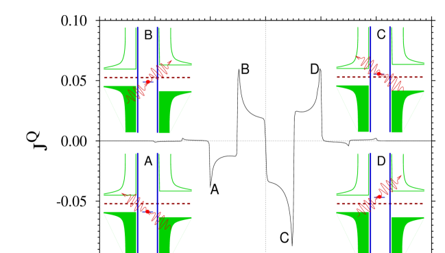
When the quantum dot is coupled to the superconductors, the pumping current due to quasiparticles can flow even when the ac-fields are applied to both sides of the leads. In the case of the normal lead, on the other hand, the electron pumping current can flow only when the ac-field is applied between the dot and one lead [8, 20]. In the normal lead case, when the ac-fields are applied to both sides of the leads, the current can not flow. Figure 1 displays the zero-bias current for unequal superconducting gap energies in the two leads. In this case, since the external frequency is smaller than the gap, the single photon processes are suppressed, and two photon processes become the dominant one because of the BCS gap. The sharp peak of the current induced by the oscillating field reflects the singularity of the BCS density of states. The sharp peaks can give rise to a good spectroscopic resolution. This suggests that a S-QD-S system can be utilized as a potentially good photo-electron device. Electron transmission processes are depicted in the inset of the Fig.1. Note that the direction and the magnitude of the current change as the level position in the quantum dot varies.

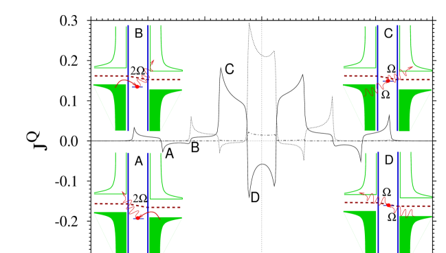
Figure 2 shows photon pumping of the current for two identical superconductors, when a small dc voltage is applied to the system. One can clearly see the negative current in some regions of parameters ($\mathsf{A,D}$), which means the negative differential conductance arises due to the photon pumping of the current. The dominant tunneling processes for $\Omega=1.5\Delta$ are depicted in the inset for several values of $\varepsilon_{\sigma}$. In regions $\mathsf{A}$ and $\mathsf{B}$ the two-photon process becomes dominant, whereas a single photon photon processes dominates, giving rise to a greater current, if the dot level lies in between the BCS gaps ($\mathsf{C,D}$). It is noteworthy that the direction and the amplitude of the current change depending on the external frequency. As one can see in the Fig.2, the direction of the current differs for different frequencies of $\Omega=0.5\Delta$, $1.0\Delta$ and $1.5\Delta$.

IV Photon-assisted Andreev Current

In the present section we will investigate the Andreev resonant tunneling through a strongly correlated quantum dot coupled to a normal metal and to a superconductor [21, 22]. We consider that an ac voltage is applied between the normal metallic lead and the quantum dot only. Generalizing the ansatz of Ng[23] to the case of a superconducting lead[21], (which leads to current conservation,) the time averaged current in the presence of sinusoidal external ac voltage on the normal lead can be obtained from Eq.(17) considering the Andreev reflections,

$$J^{A}_{\alpha}=\frac{ie}{\hbar}\!\int\!\frac{d\varepsilon}{2\pi}{\mathrm{T}r}\Big{\{}{\mathchoice{{\hbox{\boldmath$\displaystyle\sigma$}}}{{\hbox{\boldmath$\textstyle\sigma$}}}{{\hbox{\boldmath$\scriptstyle\sigma$}}}{{\hbox{\boldmath$\scriptscriptstyle\sigma$}}}}\!_{z}{\mathbf{G}}^{r}_{\sigma}(\varepsilon)[{\mathchoice{{\hbox{\boldmath$\displaystyle\Sigma$}}}{{\hbox{\boldmath$\textstyle\Sigma$}}}{{\hbox{\boldmath$\scriptstyle\Sigma$}}}{{\hbox{\boldmath$\scriptscriptstyle\Sigma$}}}}^{r}(\varepsilon),{\mathbf{K}}^{\alpha}_{N}(\varepsilon)]{\mathbf{G}}^{a}_{\sigma}(\varepsilon)\Big{\}},$$ (22)

where ${\mathbf{K}}^{\alpha}_{N}(\varepsilon)=\left(\begin{array}[]{cc}{K^{-}_{N}}(\varepsilon)&0\\ 0&{K^{+}_{N}}(\varepsilon)\end{array}\right)$ with ${K^{\pm}_{N}}(\varepsilon)=\int d\varepsilon^{\prime}\,{\mit\Gamma}^{\alpha}\,f_{\alpha}(\varepsilon^{\prime})\,Q^{\pm}_{\alpha}(\varepsilon-\varepsilon^{\prime})$. In obtaining the Andreev current we have assumed that the ac voltage difference is applied only on the normal side and that the noninteracting self-energies are in the limit $\Omega,k_{B}T,eV\ll\Delta,U$. In the absence of the ac voltage, our equation of (22) can be shown to be reduced to the current formula derived by Fazio and Raimondi[21]. The Green’s functions can be solved by the equation of motion technique, taking into account Kondo-like correlations[24]. In the infinite $U$ limit the Green’s function matrix has the form

$$\left(\mathchoice{{\hbox{\boldmath$\displaystyle\cal E$}}}{{\hbox{\boldmath$\textstyle\cal E$}}}{{\hbox{\boldmath$\scriptstyle\cal E$}}}{{\hbox{\boldmath$\scriptscriptstyle\cal E$}}}-\mathchoice{{\hbox{\boldmath$\displaystyle\cal E$}}}{{\hbox{\boldmath$\textstyle\cal E$}}}{{\hbox{\boldmath$\scriptstyle\cal E$}}}{{\hbox{\boldmath$\scriptscriptstyle\cal E$}}}_{\sigma}-\mathchoice{{\hbox{\boldmath$\displaystyle\Sigma$}}}{{\hbox{\boldmath$\textstyle\Sigma$}}}{{\hbox{\boldmath$\scriptstyle\Sigma$}}}{{\hbox{\boldmath$\scriptscriptstyle\Sigma$}}}^{r}(\varepsilon)\right){\mathbf{G}}^{r}_{\sigma}(\varepsilon)=\mathchoice{{\hbox{\boldmath$\displaystyle 1$}}}{{\hbox{\boldmath$\textstyle 1$}}}{{\hbox{\boldmath$\scriptstyle 1$}}}{{\hbox{\boldmath$\scriptscriptstyle 1$}}}-\langle\mathchoice{{\hbox{\boldmath$\displaystyle n$}}}{{\hbox{\boldmath$\textstyle n$}}}{{\hbox{\boldmath$\scriptstyle n$}}}{{\hbox{\boldmath$\scriptscriptstyle n$}}}\rangle,$$ (23)

where $\mathchoice{{\hbox{\boldmath$\displaystyle\cal E$}}}{{\hbox{\boldmath$\textstyle\cal E$}}}{{\hbox{\boldmath$\scriptstyle\cal E$}}}{{\hbox{\boldmath$\scriptscriptstyle\cal E$}}}_{\sigma}=\left(\begin{array}[]{cc}\varepsilon_{\sigma}&0\\ 0&-\varepsilon_{-\sigma}\end{array}\right)$ and the self-energy can be written as ${\mathbf{\Sigma}}(\varepsilon)={\mathbf{\Sigma}}^{r}_{N}(\varepsilon)+{\mathbf{\Sigma}}^{r}_{S}(\varepsilon)$, with ${\mathbf{\Sigma}}^{r}_{N}$ and ${\mathbf{\Sigma}}^{r}_{S}$ denoting the self-energy contribution from the normal metal and the superconductor, respectively. The effects of the PAT and Kondo correlations are included in ${\mathbf{\Sigma}}^{r}_{N,11}(\varepsilon)$ as [23]

$${\mathbf{\Sigma}}^{r}_{N,11}\!(\varepsilon)\!=\!\!\!\!\sum^{\infty}_{n=-\infty}\!\!\!J^{2}_{n}(\lambda_{N})\!\int\!\!\frac{d\varepsilon_{k}}{2\pi}\!\frac{{\mit\Gamma}^{N}[1+f_{N}(\varepsilon_{k})]}{\varepsilon\!-\!\varepsilon_{k}\!-\!eV\!-\!n\Omega\!+\!i0^{+}}.$$ (24)

We can confirm the time reversal symmetry that ${\mathbf{\Sigma}}^{r}_{N,22}(\varepsilon)=-{\mathbf{\Sigma}}^{r*}_{N,11}(-\varepsilon)$. In the large $\Delta$ limit ($\Omega,\varepsilon\ll\Delta$), ${\mathbf{\Sigma}}^{r}_{S}$ can be written as [21]

$${\mathbf{\Sigma}}^{r}_{S}=\left(\begin{array}[]{cc}{\mit\Gamma}^{S}\ln[W/\Delta]/2\pi&-{\mit\Gamma}^{S}/2\\ -{\mit\Gamma}^{S}/2&-{\mit\Gamma}^{S}\ln[W/\Delta]/2\pi\end{array}\right).$$ (25)

The off-diagonal terms are directly related to the Andreev transport, whereas the effect of the diagonal term renormalizes the energy level of the quantum dot as $\widetilde{\varepsilon}_{\sigma,-\sigma}=\varepsilon_{\sigma,-\sigma}+{\mit\Gamma}^{S}\ln[W/\Delta]/2\pi$ in the large $\Delta$ limit.

Differential conductance $dJ^{A}/dV$ as a function of the dc bias is shown in Fig.3. The zero-bias peak in the figure originates from the Kondo effect associated with the Andreev reflection. The enhancement of the zero-bias resonance by the superconductor is already studied [21, 22]. We find that new small peaks appear near the zero-bias peak, due to the PAT of the many-body resonance. The side peaks are located where the voltage is the multiple of $\mathbf{\Omega}/2$, instead $\Omega$, differently from the case for N-QD-N [25, 26]. This implies that the many-body resonance in the superconducting system changes from the normal Kondo resonance because of the Andreev reflection. The Kondo resonance in the superconducting system seems to have an effective charge $2e$ instead of $e$ due to the proximity effect. This proximity coupling seems to allow the side peaks at $2eV=n\Omega$ with $n$ being an integer.

V Conclusion

We have studied resonant transport through an interacting quantum dot coupled to superconductors in the presence of external microwave field. We derived a general formula of the current for this system, adopting the nonequilibrium Green’s function technique. We have seen that the singularity of BCS density of states plays an important as well as interesting role in the quasiparticle PAT. Influence of microwave fields on the resonant Andreev transport through a strongly correlated quantum dot has also been studied. In addition to a zero-bias peak due to many-body resonance, side peaks are found at the bias voltage corresponding to the multiples of the half of the ac oscillation frequency.

Acknowledgements.
This work has been supported in part by KOSEF, and STEPI, POSTECH/BSRI research fund. K. Kang acknowledges support by the Max-Planck-Society.

REFERENCES

  • [1] L. P. Kouwenhoven, C. M. Marcus, P. L. Mceuen, S. Tarucha, R. M. Westervelt, and N. S. Wingreen, in Mesoscopic Electron Transport, Proceedings of the NATO Advanced Study Institute, edited by L. Sohn, L. P. Kouwenhoven, G. Schön, (Kluwer,Dordrecht,1997) Series E, Vol. 345.
  • [2] D. Goldhaber-Gordon, H. Shtrikman, D. Mahalu, D. Abush-Magder, U. Meirav, and M. A. Kastner, Nature 391, 156 (1998); D. Goldhaber-Gordon, J. Göres, M. A. Kastner, H. Shtrikman, D. Mahalu, and U. Meirav, Phys. Rev. Lett.81, 5225 (1998).
  • [3] S. M. Cronenwett, T. H. Oosterkamp, and L. P. Kouwenhoven, Science 281, 540 (1998).
  • [4] P. K. Tien and J. R. Gordon, Phys. Rev. 129, 647 (1963).
  • [5] L. P. Kouwenhoven, S. Jauhar, J. Orenstein, P. L. McEuen, Y. Nagamune, J. Motohisa, and H. Sakaki, Phys. Rev. Lett.73, 3443 (1994); L. P. Kouwenhoven, S. Jauhar, K. McCormick, D. Dixon, P. L. McEuen, Yu. V. Nazarov, N. C. van der Vaart, and C. T. Foxon, Phys. Rev. B50, 2019 (1994).
  • [6] R. H. Blick, R. J. Haug, D. W. van der Weide, K. von Klitzing, and K. Eberl, Appl. Phys. Lett. 67, 3924 (1995).
  • [7] T. Fujisawa and S. Tarucha, Superlattices and Microstructures 21, 247 (1997).
  • [8] T. H. Oosterkamp, L. P. Kouwenhoven, A. E. A. Koolen, N. C. van der Vaart, and C. J. P. M. Harmans, Phys. Rev. Lett.78, 1536 (1997); Physica Scripta T69, 98 (1997).
  • [9] D. C. Ralph, C. T. Black and M. Tinkham, Phys. Rev. Lett.74, 3241 (1995); ibid. 78, 4087 (1997).
  • [10] A. F. Andreev, Zh. Eksp. Theor. Fiz. 46, 1823 (1964) [Sov. Phys. -JETP 19, 1228 (1964)].
  • [11] N. S. Wingreen, A. -P. Jauho, and Y. Meir, Phys. Rev. B48, 8489 (1993); A. -P. Jauho, N. S. Wingreen, and Y. Meir, Phys. Rev. B50, 5528 (1994).
  • [12] D. Rogovin and D. J. Scalapino, Ann. Phys. 86, 1 (1974); A. Barone and G. Paterno, Physics and Applications of the Josephson Effect (John Wiley & Sons, 1982) p.25.
  • [13] L. V. Keldysh, Zh. Eksp. Theor. Fiz. 47, 1515 (1964) [Sov. Phys. -JETP 20, 1018 (1965)]; C. Caroli, R. Combescot, P. Nozieres, and D. Saint-James, J. Phys. C 4, 916 (1971).
  • [14] S. N. Artemenko, A. F. Volkov and A. V. Zaitsev, Zh. Eksp. Theor. Fiz. 76, 1816 (1979) [Soviet Phys.-JETP 49, 924 (1979)].
  • [15] N. N. Bogoliubov, Nuovo Cimento 7, 794 (1958); Zh. Eksp. Theor. Fiz. 34, 58 (1958) [Soviet Phys.-JETP 7, 41 (1958)]; J. G. Valatin, Nuovo Cimento 7,843 (1958).
  • [16] A. L. Yeyati, J. C. Cuevas, A. López -Dávalos, and A. Martín-Rodero, Phys. Rev. B55, R6139 (1997).
  • [17] K. Kang, Phys. Rev. B57, 11 891 (1998).
  • [18] H. -K. Zhao, Phys. Lett. A 226, 105 (1997).
  • [19] H. Haug and A.-P. Jauho, Quantum Kinetics in Transport and Optics of Semiconductors, Springer Series in Solid State Sciences, Vol.123 (Springer, Berlin, Heidelberg 1996) p.170-178.
  • [20] C. Bruder and H. Schoeller, Phys. Rev. Lett.72, 1076 (1994).
  • [21] R. Fazio and R. Raimondi, Phys. Rev. Lett.80, 2913 (1998); P. Schwab and R. Raimondi, Phys, Rev. B 59 1637 (1999).
  • [22] K. Kang, Phys. Rev. B 58, 9641 (1998).
  • [23] Tai-kai Ng, Phys. Rev. Lett.76, 3635 (1996).
  • [24] Y. Meir and P. A. Lee, Phys. Rev. Lett.70, 2601 (1993).
  • [25] M. H. Hettler and H. Schoeller, Phys. Rev. Lett.74, 4907 (1995).
  • [26] A. Schiller and S. Hershfield, Phys. Rev. Lett.77, 1821 (1996).
Refer to caption
FIG. 1.: Zero-bias quasiparticle current of the S-QD-S in units of $e{\mit\Gamma}/\hbar$ for asymmetric gap energy; $\Delta_{L}=1.0$, $\Delta_{R}=1.5$. The other parameters taken here are ${\mit\Gamma}={\mit\Gamma}^{L}={\mit\Gamma}^{R}=0.01$, $k_{B}T=0.1$, $U=20$, $\lambda_{L}=\lambda_{R}=1.0$, $\Omega=1.0$, in units of $\Delta_{L}$. Diagrams of the inset displays the dominant two photon processes for several cases denoted by $\mathsf{A},B,C$ and $\mathsf{D}$.
Refer to caption
FIG. 2.: Photon induced pumping of the quasiparticle current for the S-QD-S in units of $e{\mit\Gamma}/\hbar$ for a small dc bias with two identical superconductors. $\mu_{L}=-\mu_{R}=eV/2$, $eV=0.5$, ${\mit\Gamma}={\mit\Gamma}^{L}={\mit\Gamma}^{R}=0.01$, $k_{B}T=0.1$, $U=20$, $\lambda_{L}=\lambda_{R}=1.0$, $\Omega=1.5$(solid line), $\Omega=1.0$(dotted line), and $\Omega=0.5$(dash-dotted line) in units of $\Delta=\Delta_{L}=\Delta_{R}$. Dominant processes with $\Omega=1.5$ are depicted in the diagrams of the inset for several values of the energy level in the QD.
Refer to caption
FIG. 3.: The differential conductance for the N-QD-S structure as a function of dc voltage in the units of $4e^{2}/h$ is plotted at the low temperature ($k_{B}T=1\times 10^{-4}$). In the absence of the ac field (sold line), the differential conductance has the zero-bias peak due to many-body correlation. For the ac fields of $\lambda_{N}=1$ with frequency $\Omega=0.001$ (dotted line) and $\Omega=0.0015$ (dash-dotted line), the side peaks at $2eV=n\Omega$ are found in addition to the reduced zero-bias peaks. Here ${\mit\Gamma}^{N}={\mit\Gamma}^{S}=0.02$, $\widetilde{\varepsilon}_{\sigma}=\widetilde{\varepsilon}_{-\sigma}=-0.04$ on the scale of bandwidth $W$.