[
Torque magnetometry on single-crystal high temperature superconductors near the critical temperature: a scaling approach
Abstract
Angular-dependent magnetic torque measurements performed near the critical temperature on single crystals of HgBa2CuO, LaSrCuO4, and YBa2Cu3O6.93 are scaled, following the 3D model, in order to determine the scaling function which describes the universal critical properties near . A systematic shift of the scaling function with increasing effective mass anisotropy is observed, which may be understood in terms of a 3D-2D crossover. Further evidence for a 3D-2D crossover is found from temperature-dependent torque measurements carried out in different magnetic fields at different field orientations , which show a quasi 2D “crossing region” (). The occurrence of this “crossing phenomenon” is explained in a phenomenological way from the weak dependence of the scaling function around a value . The “crossing” temperature is found to be angular-dependent. Torque measurements above reveal that fluctuations are strongly enhanced in the underdoped regime where the anisotropy is large, whereas they are less important in the overdoped regime.
pacs:
PACS: 74.25.Ha, 74.25.Bt, 05.70.Jk]
I Introduction
Angular-dependent magnetic torque measurements performed on a HgBa2CuO single crystal around were recently described within a 3D critical fluctuation model. [1, 2] When 3D critical fluctuations dominate, in a magnetic field the free energy density is given by [1]
| (1) |
is the critical amplitude of the correlation length along the direction, diverging as (), is the reduced temperature, and . is an universal constant and is an universal scaling function. It depends on the dimensionless variable which, if is applied in the plane of the sample, is given by
| (2) |
is the angle between and the axis of the sample. , is the effective mass anisotropy, and .
In a magnetic field applied in the plane of a sample with volume the magnetic torque along the axis is given by the derivative of with respect to the angle [2]
| (3) |
The functional form of the scaling function can be deduced in the following three limits:[1] for (, ), for (, ), for (, ). In the intermediate -regime was determined from angular-dependent measurements using a scaling procedure dictated by Eq. (3), as described in detail in Ref. [2]. In this paper we apply this scaling approach to single crystals of HgBa2CuO, LaSrCuO4, and YBa2Cu3O6.93 to explore the limitations of the approach arising from a large anisotropy. We assume for HgBa2CuO and for LaSrCuO4, which is reasonable due to the tetragonal structure of these compounds. For YBa2Cu3O6.93 we use (Ref. [3]).
Due to the large effective mass anisotropy most cuprates are in a 3D-2D crossover regime at temperatures slightly below where becomes smaller than the interlayer distance .[4] In the samples investigated the anisotropy values reach up to . These large values may lead to a shrinking of the temperature regime where the 3D scaling approach is applicable. The observation of a so-called “crossing point” in the temperature dependence of the magnetization can test the dimensionality of a high- material. For a 3D system the quantity is predicted to be field-independent at the critical temperature . On the other hand, in a 2D system the magnetization is predicted to be field-independent at the critical temperature of this system (Kosterlitz-Thouless transition temperature).[4] In fact, YBa2Cu3O6.93 with a moderate anisotropy only shows a 3D “crossing point” at (Ref. [5]), whereas Bi2.15Sr1.85CaCu2O with shows a rather well defined 2D “crossing point” () at .[5, 6] In the same compound 2D effects have been observed at low temperatures in muon spin rotation measurements.[7] The 2D “crossing point” () was observed in Bi2.15Sr1.85CaCu2O for fields applied along the axis, but not for fields in the plane.[4] We performed temperature-dependent torque measurements on a La1.914Sr0.086CuO4 crystal with to investigate the 2D “crossing point” in this material. The measurements were carried out at different angles in order to clarify the angular dependence of the “crossing” phenomenon.
Although an enhanced anisotropy may lead to a shrinking of the the 3D scaling temperature region, it increases the importance of fluctuation effects.[8, 9] Thus, fluctuation effects are assumed to be more important in underdoped samples showing a large anisotropy. From angular-dependent torque measurements performed above we determined the doping dependence of fluctuation effects in LaSrCuO4 compounds with different Sr contents ranging from the underdoped to the overdoped regime.
II Experimental details
The HgBa2CuO single crystals were grown using a high-pressure growth technique.[10] Oxygen annealing resulted in two crystals with and , respectively. The LaSrCuO4 samples were cut from single crystals grown by the traveling-solvent-floating-zone method with different nominal Sr compositions.[11, 12] The Sr contents of the samples were determined by an electron-probe-micro-analysis to be , , , , and , respectively. Angular-dependent torque data obtained on the YBa2Cu3O6.93 sample used in Ref. [3] were reanalyzed for this work.
The HgBa2CuO and LaSrCuO4 single crystals had typical dimensions of (g). They were mounted on a piezoresistive torque sensor between the poles of a conventional NMR-magnet with a maximum field of 1.5 T.[13] The magnetic torque acting on the magnetization of the sample was measured as a function of the angle at different constant field strengths and temperatures below and above . Only data showing reversible behavior were used for the analysis. The reversible regime was partly extended using an AC field perpendicular to to enhance relaxation processes. [14] From these reversible angular-dependent torque data the scaling function was determined for each sample.
Temperature-dependent measurements were performed on the La1.914Sr0.086CuO4 crystal for fields , , , , , and T at angles , , , , , and to study the “crossing point” phenomenon. The torque signal was continuously recorded upon cooling the sample in the applied field at a cooling rate of K/s. The measurements were only possible by compensating the strongly temperature-dependent background of the piezoresistive torque sensor by a second cantilever placed near the sample.[13] In fact, in the temperature regime , where these measurements were performed, no temperature-dependent signal was observed in zero field, pointing towards an almost perfect compensation.
The same compensation method was also used for the angular-dependent measurements where it reduced the angular-dependent magnetoresistive background of the cantilever drastically. The LaSrCuO4 samples with concentrations were measured using the cantilever in the so-called torsion mode where a torsion of the sensor around its long axis is measured by a difference in the resistance of the two piezoresistive paths integrated in the outer two legs of the lever.[13] In this differential mode no additional compensation lever is needed, and no angular dependence of the magnetoresistance is observed due to the fact that the magnetic field is always perpendicular to the main current path of the cantilever. This was especially advantageous for angular-dependent measurements, performed above in order to determine the temperature where the diamagnetic signal arising from superconducting fluctuations exactly compensates the normal paramagnetic background of the sample.
III Scaling of the angular-dependent data
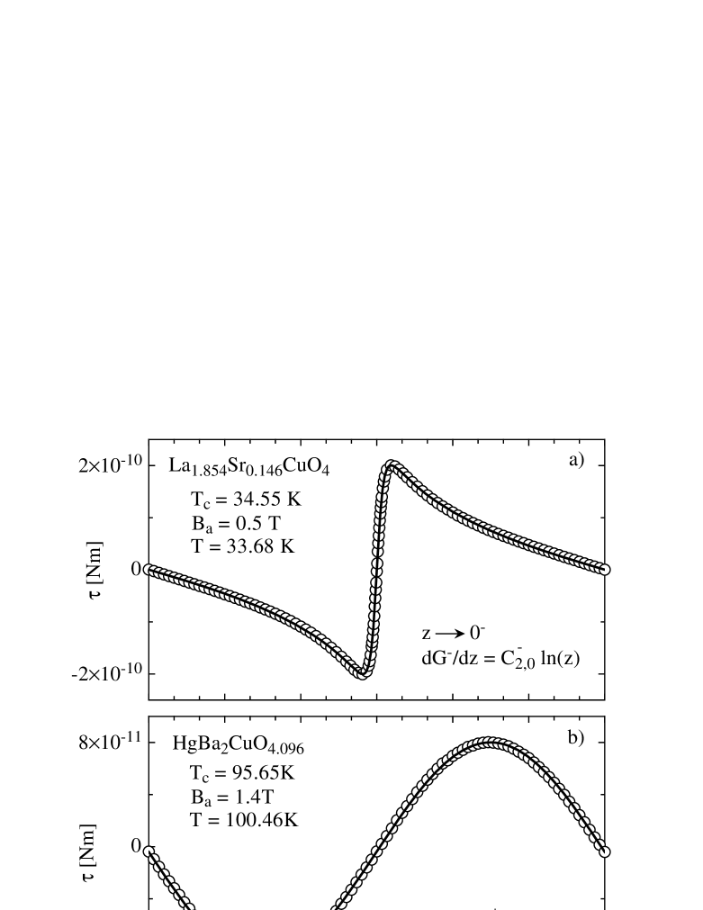
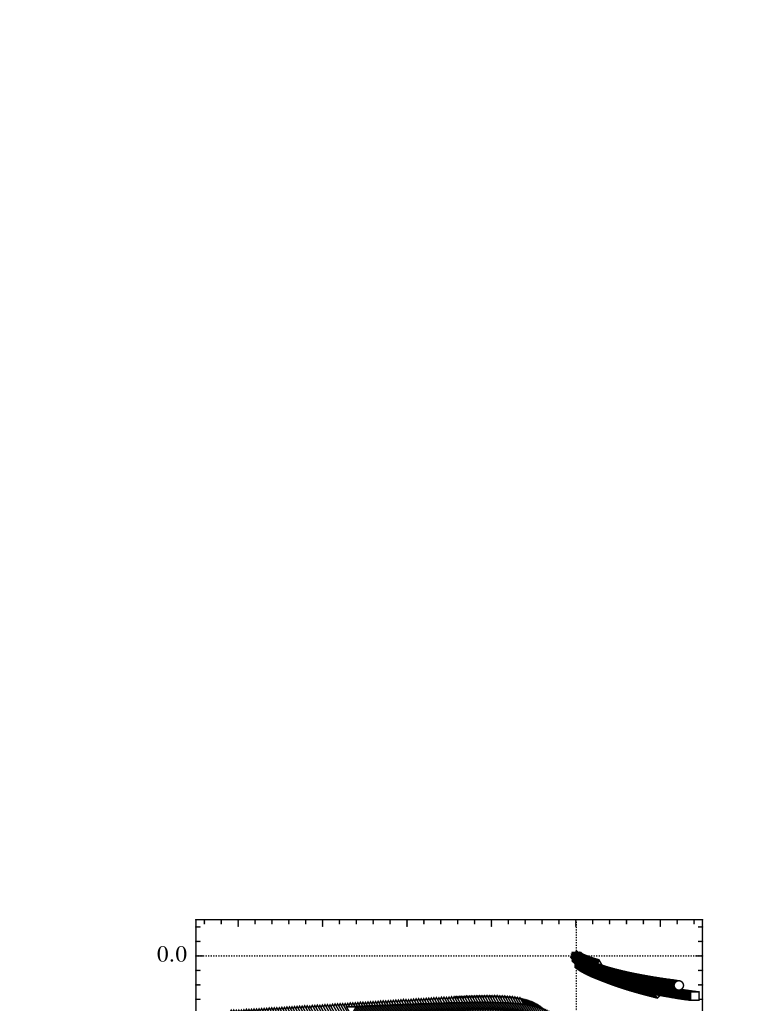
Angular-dependent torque data recorded in the three limits , , and , where the analytical form of can be deduced, are displayed in Fig. 1. The data are well described by the limiting behavior of the scaling function in the corresponding limits. For six samples with varying anisotropy the scaling procedure outlined in Ref. [2] was applied to the angular-dependent data in order to determine the scaling function . The normal paramagnetic background of the sample was determined from measurements performed above (cf. Section V) and subtracted from the data. The effective mass anisotropy and the critical amplitude of the correlation length were determined from angular-dependent measurements performed below in the low regime where [Fig. 1(a)]. In this limit the 3D form of the angular dependence of the torque coincides with the prediction of the 3D anisotropic London model.[15] Equation (3) was then resolved for using the values obtained for and . was iteratively adjusted in steps of K in order to get the best overlap of scaled curves. For , was calculated using the universal relation .
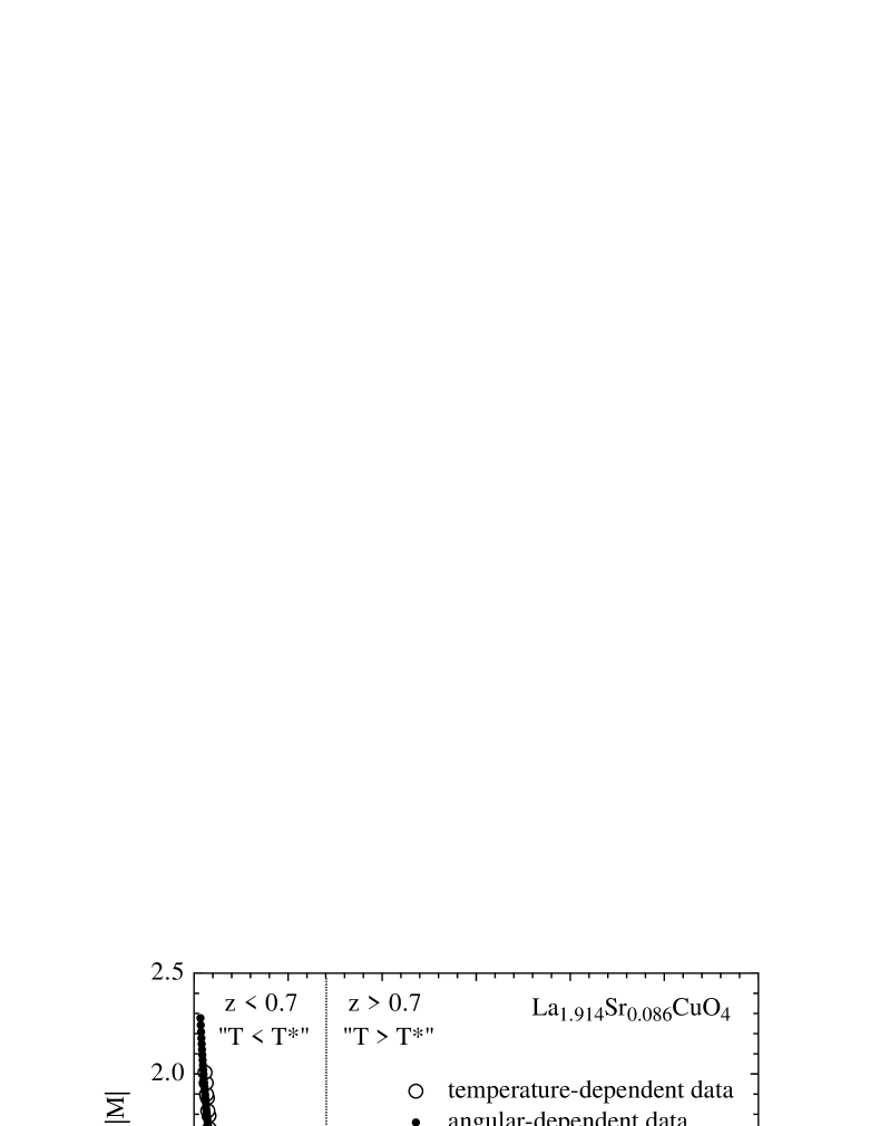
The specific heat universal constants , and critical amplitudes ratio were taken from Ref. [16]. The scaling functions obtained for all six samples are plotted in Fig. 2 as a function of .
The qualitative behavior of is the same for all samples. Especially, for the crossover from the dependence to the dependence is clearly seen for all compounds. It occurs around . All scaled data lie within an interval of 80%. This scattering partly reflects the experimental errors in performing the scaling procedure. An initial uncertainty arises from the paramagnetic background of the sample which is determined at temperatures far above and assumed to adopt the same value at temperatures around . For temperatures very close to , where the torque signal arising from superconductivity is of the same order of magnitude as the paramagnetic background, any uncertainty in determining this background can have a rather large effect. Secondly, inhomogeneities within the samples will lead to finite size effects. Talking in terms of a distribution of , will be overestimated if
the scaling procedure is performed using one single value. This overestimation comes from parts of the sample having a slightly higher and therefore giving a larger contribution to the measured torque signal. Indeed, as seen in Fig. 2 obtained for YBa2Cu3O6.93, the sample with the sharpest transition, adopts the smallest values. A third uncertainty is coming from the volume which is somewhat problematic to determine for such small samples. Finally, a crucial parameter for the scaling procedure is the correlation length amplitude which has to be determined from measurements performed in the limit . Since torque measurements cannot be carried out in very low magnetic fields where the sensitivity is not high enough, the only possibility to reach this limit is to reduce the temperature. The width of the 3D scaling temperature regime, where the temperature dependence of the correlation length is given as , is determined by corrections to scaling. For anisotropic systems, being in a 3D-2D crossover regime, the amplitudes of the correction terms can become rather large.[17] This may lead to a shrinking of the temperature regime where 3D scaling is applicable. The correction amplitudes are not known a priori and vary between different samples,
| sample | [K] | [Å] | [Å] | |
|---|---|---|---|---|
| YBa2Cu3O6.93 | 93.35(5) | 7.5(5) | 13(2) | 1130(90) |
| HgBa2CuO4.108 | 88.80(5) | 20.5(8) | 29(4) | 1000(80) |
| HgBa2CuO4.096 | 95.65(5) | 29(1) | 26(4) | 780(80) |
| La1.854Sr0.146CuO4 | 34.55(5) | 18.4(6) | 30(4) | 1720(130) |
| La1.914Sr0.086CuO4 | 21.60(5) | 46(1) | 79(12) | 2230(170) |
| La1.920Sr0.080CuO4 | 19.35(5) | 51(1) | 101(15) | 2530(190) |
therefore only the 3D temperature dependence was taken into account for our analysis. The critical amplitude of the correlation length determined from measurements performed at different temperatures and fields, such that was rather well fulfilled for each measurement, showed a scattering of about 20%. Therefore, we estimate the error in to be 15%, leading to the same error in and to an error of 30% in .
As observed in Fig. 2, the scaling functions obtained for the samples investigated deviate systematically with increasing from that of YBa2Cu3O6.93, the sample with the smallest anisotropy. The amplitudes of the correction terms mentioned above depend on how gradually the crossover occurs [17], and is a measure for quasi 2D behavior of the cuprates. Therefore, it is plausible that the corrections to 3D scaling depend systematically on the anisotropy are getting more important with increasing . However, there are not enough data available to determine these corrections quantitatively.
The critical amplitudes obtained for all six samples from the 3D scaling approach are listed in Table I. The penetration depth amplitude is calculated using the universal relation .[1] An error of 15% was assumed for (see above) leading to an error of % for . The tendency for , , and to increase with decreasing doping in the underdoped regime, as observed in different experiments, [18, 19, 20, 21] is evident for the LaSrCuO4 samples. The anisotropy values found for LaSrCuO4 are in rather good
| universal constant | range |
|---|---|
| 0.6 to 0.8 | |
| -0.8 to -1.0 | |
| -0.3 to -0.5 |
Table II lists the range which we determined from the 3D scaling approach for the three universal constants corresponding to the three limits of (cf. Fig. 1). The largest uncertainty is found for the limit , i.e. . This may reflect the problems arising from a distribution of , as already discussed above.
IV The “crossing point” phenomenon
Taking the derivative of [Eq. (1)] with respect to the magnetic field, we find the 3D- expression for the magnetization
| (4) |
In the limit , where , Eq. (4) predicts the 3D “crossing point” () which is observed in the temperature-dependent magnetization.[5] Here we concentrate on the 2D “crossing point” (), which has been widely studied.[4, 5, 6] For , decreases with increasing field, whereas for it increases with increasing field. The same change in the field dependence of the magnetization is described by the scaling function for . , as determined by scaling the angular-dependent data, is plotted in Fig. 3 for the case of La1.914Sr0.086CuO4 (small symbols). The scaling function obtained from temperature-dependent data measured at different angles and fields is also included (large symbols). The agreement of the angular-dependent and temperature-dependent measurements is excellent. For , decreases with increasing , whereas for it increases with increasing . Let us recall the dependence of on temperature, field and angle by looking at Eq. (2). can be increased in three ways: (i) , , ; (ii) , , ; (iii) , , . Since , we recover the above crossover in the field dependence of from , if for an intermediate field of T the scaling argument adopts the value , where has its minimum, at the temperature . The situation is indicated by the vertical line in Fig. 3. Thus, we can define in a purely phenomenological way a “crossing temperature” by the condition
| (5) |
The “crossing” magnetization is then given by . From Fig. 3 it is evident that we will not observe a perfect “crossing point” (), where is exactly independent of the applied field. Indeed, at the temperature as defined by Eq. (5), for all applied fields T, and therefore .
Since decreases monotonically upon approaching from below, only for a temperature the magnetization adopts the value . However, only shows a weak dependence for and is close to . Therefore, if one looks at temperature-dependent magnetization measurements over a rather large temperature interval, a quite well defined “crossing point” will be observed for fields up to T. The situation is slightly different for fields T. In that case , and again . But shows a strong dependence for . Therefore , where , can be considerably higher than , and magnetization curves measured in fields T tend to “cross” at higher temperatures. Thus we expect to observe a “crossing region” with a width that is mainly determined by low field measurements. In fact, experiments show that the “crossing point” is actually a “crossing region”, and low field measurements lie at higher temperatures.[4]
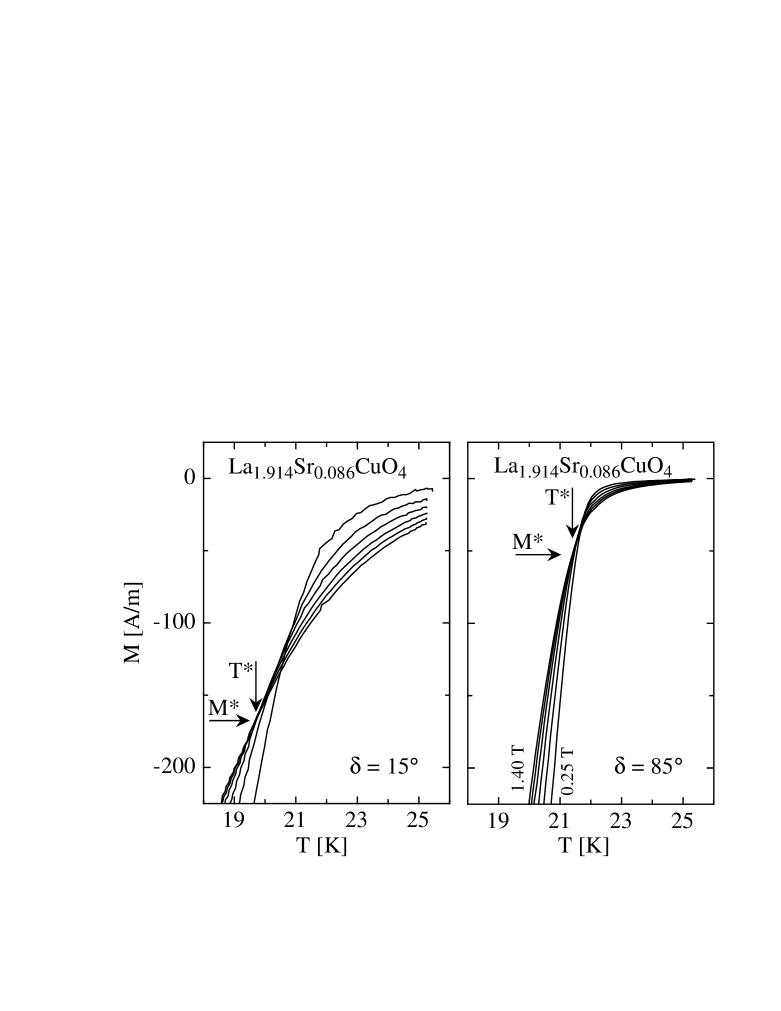
If we take the angular dependence of into account, we see that for a field orientation close to the plane of the sample, where has a minimum, Eq. (5) is fulfilled for a higher temperature . Therefore, we expect to increase with increasing in the range . Furthermore, as the temperature dependence of gets stronger upon approaching the width of the crossing region, which is determined by measurements with small , is expected to shrink for field orientations close to the plane. This trend is clearly seen in Fig. 4 where temperature-dependent measurements on La1.914Sr0.086CuO4 performed in different fields are presented for and , respectively. As indicated by the arrows, and are determined from the crossing of the magnetization curves recorded in fields T. The measurements at T and T are not taken into account.
Presuming for all orientations , one obtains from Eq. (2) an angular-dependent “crossing temperature”
| (6) |
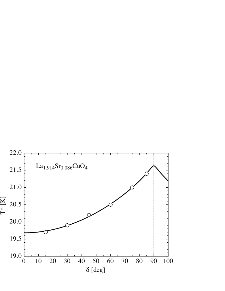
Figure 5 shows as a function of the angle . The solid line represents a least square fit to Eq. (6). The observed angular dependence of is well reproduced with the fitting parameters K and K (the anisotropy was fixed at ). With K we find the actual value of to be . Indeed, the “crossing region” is located around the -value, where adopts its minimum. Comparing the left panel to the right panel of Fig. 4, we can see that adopts a considerable higher value for than for . Figure 6 displays as a function of . The solid line is calculated by combining Eqs. (4) and (6) using K, K, , , and for (see Fig. 3). The calculated angular-dependence of is in fair agreement
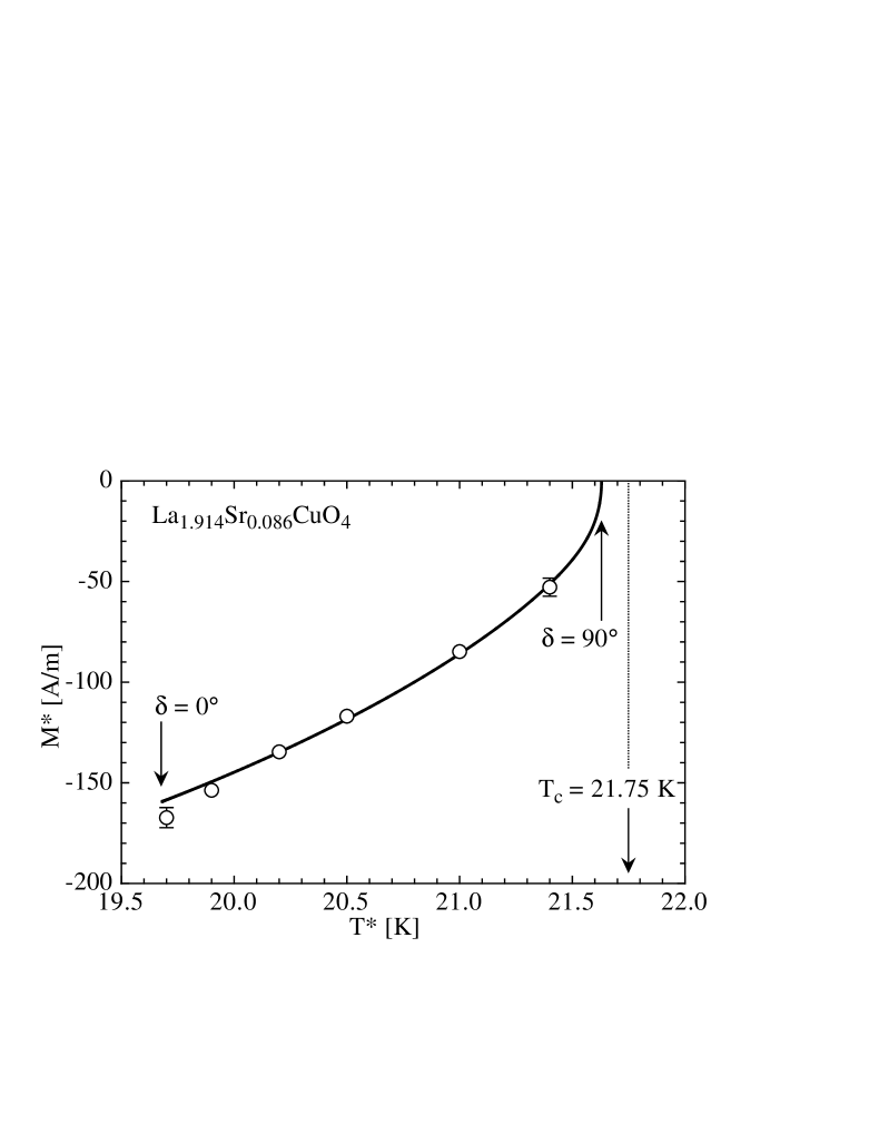
with the measured data. Figure 7 displays the dependence of on in the La1.914Sr0.086CuO4 sample. Upon turning the field towards the plane, monotonically increases from K to K (see also Fig. 5). Due to the strong temperature dependence of the magnetization in this temperature range, changes dramatically. For we find Am2, whereas it almost vanishes for , where we calculate A/m, K. Due to the small value of , it is very difficult to resolve the “crossing point” for fields applied at . Indeed, magnetization curves recorded at are found to join at rather than to “cross” slightly below (Ref. [4]).
V Torque signal above the critical temperature: importance of superconducting fluctuations
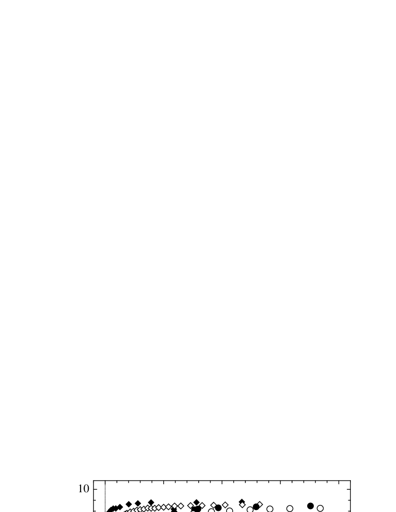
The temperature dependence of the amplitude of the signal observed for temperatures [Fig. 1(b)] yields information about the importance of superconducting fluctuations. Figure 8 shows the normalized amplitude as a function of the reduced temperature for LaSrCuO4 samples with different doping . At temperatures well above a positive, almost temperature-independent amplitude is observed. This signal is mainly due to the Van Vleck paramagnetic response of the copper ions.[22, 23] Within the investigated doping range the Van Vleck contribution is found to be independent of . In the underdoped regime, below temperatures , starts to decrease and finally vanishes at a temperature . For the amplitude is negative and increases dramatically upon approaching . The observed temperature dependence of is due to superconducting fluctuations. This is evidenced by the fact that the signal is clearly related with . Moreover, the temperature dependence of is well described by the 3D expression for
temperatures close to (Ref. [2]). With , from Eq. (3) we find
| (7) |
It is evident from this expression that is large (i.e. fluctuations are important) for large values of and . As seen from Table I, and both increase with decreasing doping in underdoped LaSrCuO4. The decrease in , which also affects , is smaller than the increase in and . Thus, from Eq. (7) we can conclude that fluctuations are important in the underdoped regime. More general, the importance of fluctuations in highly anisotropic systems is seen from the fact, that an anisotropic system can be rescaled to the isotropic case with a strongly enhanced temperature .[24] This enhancement of the rescaled temperature gives rise to strong fluctuations.
As seen in Fig. 8, in the underdoped compounds, at temperatures substantially higher than superconducting fluctuations start to play an important role and the corresponding diamagnetic signal competes the paramagnetic Van Vleck contribution. Below the fluctuation signal predominates the paramagnetic background and the overall response of the sample is of diamagnetic nature. The temperature below which deviations from the normal paramagnetic behavior are observed, provides a measure for the temperature regime where fluctuations are important. However, this temperature is not well defined. On the other hand, the temperature , where the torque signal completely vanishes, is very well defined and its value compared to yields information about the importance of superconducting fluctuations. Clearly, shifts closer to upon increasing the doping. The doping dependence of is shown in Fig. 9. This quantity is a good indicator for the importance of superconducting fluctuations at different doping levels,
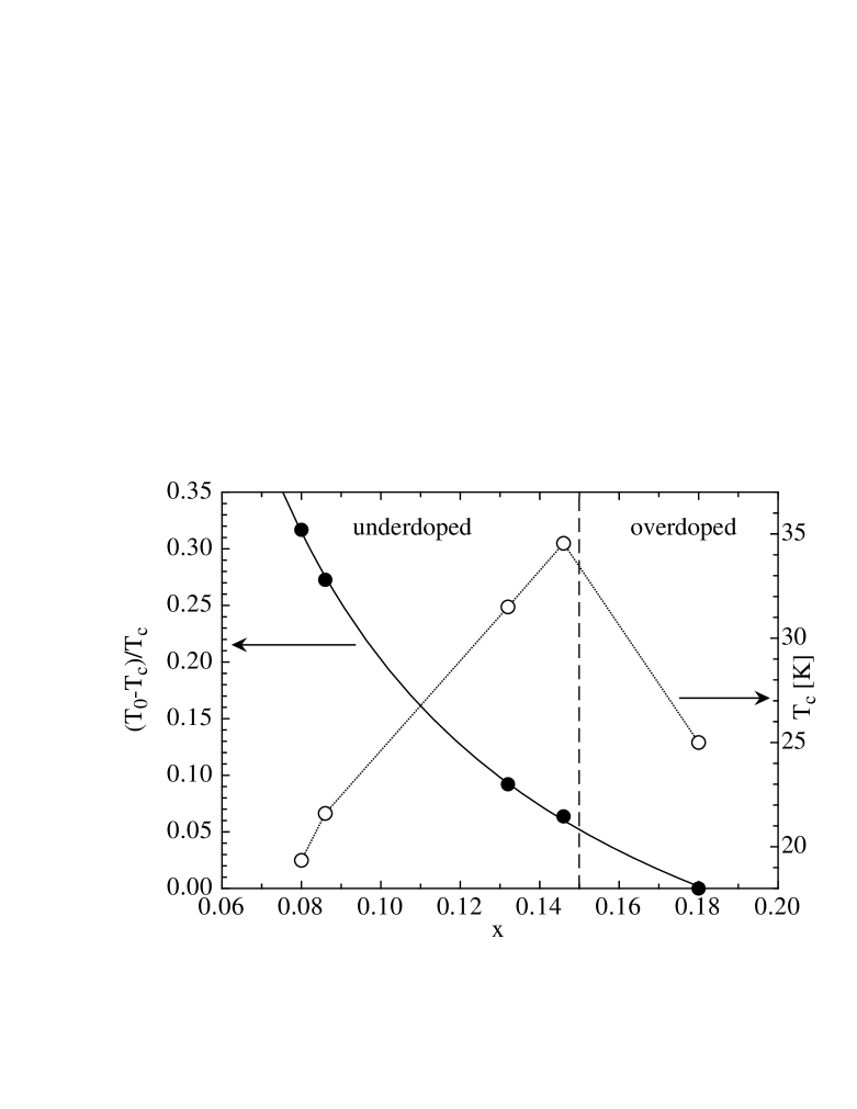
since the paramagnetic background is the same for all samples. For , at the superconducting signal already exceeds the paramagnetic background. This means that superconducting fluctuations show up over a wide temperature range in this doping regime. Indeed, fluctuations are important at least up to , as shown in Fig. 8. On the other hand, and can no longer be distinguished for ; as expected, fluctuations are less important in the overdoped regime, where is small.
VI discussion
Since the scaling function is determined experimentally, all features showing up in experiments are included in . Therefore, it is evident that the “crossing point” phenomenon can be deduced from a feature contained in the scaling function. As pointed out in Section IV, once is determined, it is possible to predict the angular dependence of and and to predict that the “crossing point” is actually a “crossing region”, spreading over a finite temperature interval. Moreover, the fact that no “crossing point” can be resolved for fields applied in the plane is explained. Note that all these predictions regarding temperature-dependent data can be easily obtained by scaling angular-dependent measurements, using the fact that all torque data recorded within a not too large temperature regime around fall onto a single curve if they are scaled according to Eq. (3). Temperature-dependent measurements performed at on the La1.914Sr0.086CuO4 single crystal showing the “crossing point” phenomenon are shown in the left panel of Fig. 10. The right panel displays the temperature-dependent magnetization at the same angles and fields, extracted from the scaling function which is obtained from three angular-dependent measurements performed below (small symbols in Fig. 3) and from one angular-dependent measurement performed above .
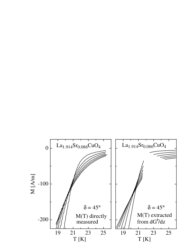
For each data point (), the corresponding temperature is calculated from using Eq. (2), afterwards is calculated using Eq. (4). Since very high values are not covered by the angular-dependent data for , temperatures very close to are not reached. Small deviations between the measured data and the calculated points for temperatures very near and above are due to finite size effects and an uncertain background correction. On the other hand, we observe a remarkable agreement between the measured and the extracted magnetization for temperatures around . For K the magnetization curves extracted from start to deviate significantly from the directly measured curves, because we leave the temperature regime where the scaling approach is applicable. This temperature region is thus estimated to be .
The investigation of the “crossing point” phenomenon is one example for the powerful possibilities of the scaling approach. Another example regarding the melting line is given in Ref. [2]. Moreover, by integrating with respect to one gets the scaling function of the singular part of the free energy density, Eq (1), where the integration constant is determined by the condition (Ref. [1]). Other quantities of interest as the specific heat can then be calculated using thermodynamic relations.
The determination of the scaling function from angular-dependent measurements is a very reliable technique, since a rotation of the sample at fixed magnetic field and temperature allows to scan over a large regime, , by only changing the well controllable parameter [Eq. (2)]. One should mention, that in order to test the expression for the 3D free energy density [Eq. (1)], it is much more convenient to investigate the magnetization or the magnetic torque than to investigate the specific heat. This is due to the fact that taking the derivative of with respect to the magnetic field or the angle (leading to the magnetization or the magnetic torque) only results in one term, whereas the double derivative of with respect to the temperature leads to six terms. On the other hand, specific heat measurements performed in zero field around yield important information about finite size effects. [25]
The occurrence of a “crossing point” in the cuprates is ascribed to a quasi 2D behavior of these materials. [4, 26, 27] As shown in this work, the same crossover in the behavior of the magnetization (i.e. a decrease of with increasing field for low temperatures and an increase of with increasing field for high temperatures) also exists in the 3D model. This is seen by recalling again the two limits and where and , respectively. The square root dependence of for is a characteristic property of the 3D model. As seen from Eq. (3), a finite torque at is only possible for . The resulting very unusual angular dependence of the magnetic torque near is indeed observed [cf. Fig. 1(c)] and gives very strong evidence for 3D critical fluctuations close to . On the other hand, the low limit is mainly covered by torque data recorded for angles close to the plane, where the cuprates show 3D behavior.[2, 4, 7] However, it is not clear whether the “crossing region” () can be described as an exact 3D behavior, as well. If we attribute the “crossing point” to a quasi 2D behavior, this means that for intermediate values includes data recorded in a region where quasi 2D effects become important. One would then still expect one single 3D scaling function for all samples at temperatures very close to , i.e. for large values of . However, as already mentioned above, in this temperature regime different distributions in the samples lead to discrepancies of the scaling functions. In addition, the overlap of the scaled curves occurs in the intermediate regime, i.e. the scaling procedure is optimized for a region where the cuprates may not show exact 3D behavior. This might explain the systematic shift of with increasing anisotropy observed in Fig. 2. On the other hand, deviations from a 3D behavior are not too large since it is still possible to perform a scaling procedure based on the 3D model for each sample. Note, that due to restrictions of our magnet all measurements are performed in relatively low fields T. For all samples used in this work, the crossover field , above which the pancake vortices loose their correlation along the axis and thus show quasi 2D behavior,[4, 7] is larger than T. It is well possible, that for higher fields T 2D effects are much more important, and the 3D scaling approach, restricted to a narrow temperature regime around , breaks down for .
From Fig. 9 it is evident that fluctuation effects play a more important role in the underdoped regime of high- systems whereas they are less important in the overdoped regime. If we take into account that the anisotropy increases in the underdoped regime (see Table I and Refs. [18, 19]), that strongly underdoped compounds show 2D scaling behavior[28] and that fluctuations are strong in quasi 2D systems,[9] our measurements are consistent with the picture that highly overdoped high- cuprates may be treated within a 3D mean field theory, whereas strongly underdoped compounds are dominated by (2D) fluctuations.[28] Although an enhanced anisotropy increases the fluctuation regime, it may shrink the temperature regime where 3D scaling is applicable, due to enhanced corrections to scaling. It is worth to point out, that the occurrence of superconducting fluctuations above clearly implies that pairs exist above . Thus, in the underdoped regime pairs are present at least up to .
In summary we applied a 3D scaling approach to a variety of high- cuprates with different anisotropy . For each sample, scaled angular-dependent torque data recorded near fall onto the scaling function . Starting from this scaling function, it is possible to predict the behavior of different physical quantities, such as magnetization, specific heat etc. close to , using the fact that all measurements fall onto the same curve , provided they are scaled properly. We are able to predict an angular-dependent “crossing temperature” where the magnetization seems to be independent of the applied field. Investigations of the angular-dependent torque data recorded at on LaSrCuO4 single crystals with different doping show that fluctuation effects are more important in the underdoped regime. This is understood in terms of an enhanced anisotropy in the underdoped samples and supports the picture that a 3D mean field treatment of high- materials is applicable in the highly overdoped regime, whereas strongly underdoped compounds are dominated by (2D) fluctuations. The scaling functions obtained for samples with higher deviate systematically with increasing anisotropy from that obtained for the sample with the lowest value. This may be understood by the fact that the layered high- cuprates show a 3D-2D crossover with decreasing temperature. This crossover enhances the corrections to scaling and reduces the 3D critical regime.
acknowledgments
The authors would like to thank K. Kwok for providing the YBa2Cu3O7 sample. Fruitful discussions with C. Rossel are deeply acknowledged. This work was partly supported by the Swiss National Science Foundation, and by NEDO and CREST/JST (Japan). One of the authors (T.S.) would like to thank JSPS for financial support.
REFERENCES
- [1] T. Schneider, J. Hofer, M. Willemin, J.M. Singer, and H. Keller, Eur. Phys. J. B 3, 413 (1998).
- [2] J. Hofer, T. Schneider, J.M. Singer, M. Willemin, H. Keller, C. Rossel, and J. Karpinski, Phys. Rev. B 60, 1332 (1999).
- [3] M. Willemin, A. Schilling, H. Keller, C. Rossel, J. Hofer, U. Welp, W.K. Kwok, R.J. Olsson, and G.W. Crabtree, Phys. Rev. Lett. 81, 4236 (1998).
- [4] T. Schneider and J.M. Singer, Physica C 313, 188 (1999).
- [5] A. Junod, K.-Q. Wang, T. Tsukamoto, G. Triscone, B. Revaz, E. Walker, and J. Muller, Physica C 229, 209 (1994).
- [6] P.H. Kes, C.J. Van der Beek, M.P. Maley, M.E. McHenry, D.A. Huse, M.J.V. Menken, and A.A. Menovsky, Phys. Rev. Lett. 67, 2383 (1991).
- [7] C.M. Aegerter, J. Hofer, I.M. Savić, H. Keller, S.L. Lee, C. Ager, S.H. Lloyd, and E.M. Forgan, Phys. Rev. B 57, 1253 (1998).
- [8] D.S. Fisher, M.P.A. Fisher, and D.A. Huse, Phys. Rev. B 43, 130 (1991).
- [9] N. Goldenfeld, in Lectures on Phase Transitions and the Renormalization Group, Addison-Wesley, Reading, (1992).
- [10] J. Karpinski, G.I. Meijer, H. Schwer, R. Molinski, E. Kopnin, K. Conder, M. Angst, J. Jun, S. Kazakov, A. Wisniewski, R. Puzniak, J. Hofer, V. Alyoshin, and A. Sin, Supercond. Sci. Technol. 12, R153 (1999).
- [11] T. Kimura, K. Kishio, T. Kobayashi, Y. Nakayama, N. Motohira, K. Kitazawa, and K. Yamafuji, Physica C 192, 247 (1992).
- [12] T. Sasagawa, K. Kishio, Y. Togawa, J. Shimoyama, and K. Kitazawa, Phys. Rev. Lett. 80, 4297 (1998).
- [13] M. Willemin, C. Rossel, J. Brugger, M.H. Despont, H. Rothuizen, P. Vettiger, J. Hofer, and H. Keller, J. Appl. Phys. 83, 1163 (1998).
- [14] M. Willemin, C. Rossel, J. Hofer, H. Keller, A. Erb, and E. Walker, Phys. Rev. B 58, R5940 (1998).
- [15] D.E. Farrell, C.M. Williams, S.A. Wolf, N.P. Bansal, and V.G. Kogan, Phys. Rev. Lett. 61, 2805 (1988).
- [16] C. Bervillier, Phys. Rev. B 14, 4964 (1976).
- [17] M.E. Fisher, Rev. Mod. Phys. 46, 597 (1974).
- [18] T.R. Chien, W.R. Datars, B.W. Veal, A.P. Paulikas, P. Kostic, C. Gu, and Y. Jiang, Physica C 229, 273 (1994).
- [19] J. Hofer, J. Karpinski, M. Willemin, G. I. Meijer, E. M. Kopnin, R. Molinski, H. Schwer, C. Rossel, and H. Keller, Physica C 297 , 103 (1998).
- [20] Y. Jaccard, T. Schneider, J. P. Locquet, E. J. Williams, P. Martinoli, and Ø. Fischer, Europhys. Lett. 34, 281 (1996).
- [21] T. Schneider and H. Keller, Int. J. Mod. Phys. 8, 487 (1993).
- [22] W.C. Lee and D.C. Johnson, Phys. Rev. B 41, 1904 (1990).
- [23] F. Mehran, T.R. McGuire, and G.V. Chandrashekar, Phys. Rev. B 41, R11 583 (1990).
- [24] G. Blatter, M.V. Feigel’man, V.B. Geshkenbein, A.I. Larkin, and V.M. Vinokur, Rev. Mod. Phys. 66, 1125 (1994).
- [25] T. Schneider and J.M. Singer (cond-mat/9911352).
- [26] L.N. Bulaevskii, M. Ledvij, and V.G. Kogan, Phys. Rev. Lett. 68, 3773 (1992).
- [27] Z. Teŝanović, L. Xing, L. Bulaevskii, Q. Li, and M. Suenaga, Phys. Rev. Lett. 69, 3563 (1992).
- [28] T. Schneider, Acta Phys. Pol. A 91, 203 (1997).