Economic Fluctuations and Diffusion

Abstract

Stock price changes occur through transactions, just as diffusion in physical systems occurs through molecular collisions. We systematically explore this analogy [1] and quantify the relation between trading activity — measured by the number of transactions $N_{\Delta t}$ — and the price change $G_{\Delta t}$ for a given stock, over a time interval $[t,\,t+\Delta t]$. To this end, we analyze a database documenting every transaction for 1000 US stocks over the two-year period 1994–1995 [2]. We find that price movements are equivalent to a complex variant of diffusion, where the diffusion coefficient fluctuates drastically in time. We relate the analog of the diffusion coefficient to two microscopic quantities: (i) the number of transactions $N_{\Delta t}$ in $\Delta t$, which is the analog of the number of collisions and (ii) the local variance $w^{2}_{\Delta t}$ of the price changes for all transactions in $\Delta t$, which is the analog of the local mean square displacement between collisions. We study the distributions of both $N_{\Delta t}$ and $w_{\Delta t}$, and find that they display power-law tails. Further, we find that $N_{\Delta t}$ displays long-range power-law correlations in time, whereas $w_{\Delta t}$ does not. Our results are consistent with the interpretation that the pronounced tails of the distribution of $G_{\Delta t}$ [3, 4, 5, 6, 7, 8, 9, 10, 11, 12] are due to $w_{\Delta t}$, and that the long-range correlations previously found [13, 14, 15, 16, 17] for $|G_{\Delta t}|$ are due to $N_{\Delta t}$.

Consider the diffusion [18, 19, 20] of an ink particle in water. Starting out from a point, the ink particle undergoes a random walk due to collisions with the water molecules. The distance covered by the particle after a time $\Delta t$ is

$$x_{\Delta t}=\sum_{i=1}^{N_{\Delta t}}\,\delta x_{i}\,,$$ (2)

where $\delta x_{i}$ are the distances that the particle moves in between collisions, and $N_{\Delta t}$ denotes the number of collisions during the interval $\Delta t$. The distribution $P(x_{\Delta t})$ is Gaussian with a variance $\langle x_{\Delta t}^{2}\rangle=N_{\Delta t}\,w_{\Delta t}^{2}$, where the local mean square displacement $w_{\Delta t}^{2}\equiv\langle(\delta x_{i})^{2}\rangle$ is the variance of the individual steps $\delta x_{i}$ in the interval $[t,\,t+\Delta t]$.

For the classic diffusion problem considered above: (i) the probability distribution $P(N_{\Delta t})$ is a “narrow” Gaussian, i.e., has a standard deviation much smaller than the mean $\langle N_{\Delta t}\rangle$, (ii) the time between collisions of an ink particle are not strongly correlated, so $N_{\Delta t}$ at any future time $t+\,\tau$ depends at most weakly on $N_{\Delta t}$ at time $t$—i.e., the correlation function $\langle N_{\Delta t}(t)N_{\Delta t}(t+\tau)\rangle$ has a short-range exponential decay, (iii) the distribution $P(w_{\Delta t})$ is also a narrow Gaussian, (iv) the correlation function $\langle w_{\Delta t}(t)w_{\Delta t}(t+\tau)\rangle$ has a short-range exponential decay and (v) the variable $\epsilon\equiv x_{\Delta t}/(w_{\Delta t}\sqrt{N_{\Delta t}})$ is uncorrelated and Gaussian-distributed. These conditions result in $x_{\Delta t}$ being Gaussian distributed and weakly correlated.

An ink particle diffusing under more general conditions would result in a quite different distribution of $x_{\Delta t}$, such as in a bubbling hot spring, where the characteristics of bubbling depend on a wide range of time and length scales. In the following, we will present empirical evidence that the movement of stock prices is equivalent to a complex variant of classic diffusion, specified by the following conditions: (i) $P(N_{\Delta t})$ is not a Gaussian, but has a power-law tail, (ii) $N_{\Delta t}$ has long-range power-law correlations, (iii) $P(w_{\Delta t})$ is not a Gaussian, but has a power-law tail, (iv) the correlation function $\langle w_{\Delta t}(t)w_{\Delta t}(t+\tau)\rangle$ is short ranged, and (v) the variable $\epsilon\equiv x_{\Delta t}/(w_{\Delta t}\sqrt{N_{\Delta t}})$ is Gaussian distributed and short-range correlated. Under these conditions, the statistical properties of $x_{\Delta t}$ will depend on the exponents characterizing these power laws.

Just as the displacement $x_{\Delta t}$ of a diffusing ink particle is the sum of $N_{\Delta t}$ individual displacements $\delta x_{i}$, so also the stock price change $G_{\Delta t}$ is the sum of the price changes $\delta p_{i}$ of the $N_{\Delta t}$ transactions in the interval $[t,t+\Delta t]$,

$$G_{\Delta t}=\sum_{i=1}^{N_{\Delta t}}\delta p_{i}\,.$$ (3)

Figure 1a shows $N_{\Delta t}$ for classic diffusion and for one stock (Exxon Corporation). The number of trades for Exxon displays several events the size of tens of standard deviations and hence is inconsistent with a Gaussian process [21, 22, 23, 24, 25, 26].

(i) We first analyze the distribution of $N_{\Delta t}$. Figure 1c shows that the cumulative distribution of $N_{\Delta t}$ displays a power-law behavior $P\{N>x\}\sim x^{-\beta}$. For the 1000 stocks analyzed, we obtain a mean value $\beta=3.40\pm 0.05$ (Fig. 1d). Note that $\beta>2$ is outside the Lévy stable domain $0<\beta<2$.

(ii) We next determine the correlations in $N_{\Delta t}$. We find that the correlation function $\langle N_{\Delta t}(t)N_{\Delta t}(t+\tau)\rangle$ is not exponentially decaying as in the case of classic diffusion, but rather displays a power-law decay (Fig. 1e,f). This result quantifies the qualitative fact that if the trading activity ($N_{\Delta t}$) is large at any time, it is likely to remain so for a considerable time thereafter.

(iii) We then compute the variance $w_{\Delta t}^{2}\equiv\langle(\delta p_{i})^{2}\rangle$ of the individual changes $\delta p_{i}$ due to the $N_{\Delta t}$ transactions in the interval $[t,\,t+\Delta t]$ (Fig. 2a). We find that the distribution $P(w_{\Delta t})$ displays a power-law decay $P\{w_{\Delta t}>x\}\sim x^{-\gamma}$ (Fig. 2b). For the 1000 stocks analyzed, we obtain a mean value of the exponent $\gamma=2.9\pm 0.1$ (Fig. 2c).

(iv) Next, we quantify correlations in $w_{\Delta t}$. We find that the correlation function $\langle w_{\Delta t}(t)\,w_{\Delta t}(t+\tau)\rangle$ shows only weak correlations (Fig. 2d,e). This means that $w_{\Delta t}$ at any future time $t+\tau$ depends at most weakly on $w_{\Delta t}$ at time $t$.

(v) Consider now $\delta p_{i}$ chosen only from the interval $[t,\,t+\Delta t]$, and let us hypothesize that these $\delta p_{i}$ are mutually independent and with a common distribution $P(\delta p_{i}|t\in[t,t+\Delta t])$ having a finite variance $w_{\Delta t}^{2}$. Under this hypothesis, the central limit theorem implies that the ratio

$$\epsilon\equiv{G_{\Delta t}\over w_{\Delta t}\sqrt{N_{\Delta t}}}$$ (4)

must be a Gaussian-distributed random variable with zero mean and unit variance [27]. Indeed, for classic diffusion, $x_{\Delta t}/(w_{\Delta t}\sqrt{N_{\Delta}})$ is Gaussian-distributed and uncorrelated (Fig. 3a). We confirm this hypothesis by analyzing (a) the distribution $P(\epsilon)$, which we find to be consistent with Gaussian behavior (Fig. 3b), and (b) the correlation function $\langle\epsilon(t)\,\epsilon(t+\tau)\rangle$, for which we find only short-range correlations (Fig. 3c,d).

Thus far, we have seen that the data for stock price movements support the following results: (i) the distribution of $N_{\Delta t}$ decays as a power-law, (ii) $N_{\Delta t}$ has long-range correlations, (iii) the distribution of $w_{\Delta t}$ decays as a power-law, (iv) $w_{\Delta t}$ displays only weak correlations, and (v) the price change $G_{\Delta t}$ at any time is consistent with a Gaussian-distributed random variable [21, 22, 23, 24, 28, 29, 30, 31] with a time-dependent variance $N_{\Delta t}\,w_{\Delta t}^{2}$, that is, the variable $\epsilon\equiv G_{\Delta t}/(w_{\Delta t}\sqrt{N_{\Delta t}})$ is Gaussian-distributed and uncorrelated.

Next, we explore the implications of our empirical findings. Namely, we show how the statistical properties [5, 6, 7, 8, 9, 10, 11, 12, 13, 14, 15] of price changes $G_{\Delta t}$ can be understood in terms of the properties of $N_{\Delta t}$ and $w_{\Delta t}$. We will argue that the pronounced tails of the distribution of price changes [5, 6, 7, 8, 9, 10, 11, 12] are largely due to $w_{\Delta t}$ and the long-range correlations previously found [13, 14, 15, 16, 17] for $|G_{\Delta t}|$ are largely due to the long-range correlations in $N_{\Delta t}$. By contrast, in classic diffusion $N_{\Delta t}$ and $w_{\Delta t}$ do not change the Gaussian behavior of $x_{\Delta t}$ because they have only uncorrelated Gaussian-fluctuations [21, 27].

Consider first the distribution of price changes $G_{\Delta t}$, which decays as a power-law $P\{G_{\Delta t}>x\}\sim x^{-\alpha}$ with an exponent $\alpha\approx 3$ [8, 9, 10, 11, 12]. Above, we reported that the distribution $P\{N_{\Delta t}>x\}\sim x^{-\beta}$ with $\beta\approx 3.4$ (Fig. 1c,d). Therefore, $P\{\sqrt{N_{\Delta t}}>x\}\sim x^{-2\beta}$ with $2\beta\approx 6.8$. Equation (4) then implies that $N_{\Delta t}$ alone cannot explain the value $\alpha\approx 3$. Instead, $\alpha\approx 3$ must arise from the distribution of $w_{\Delta t}$, which indeed decays with approximately the same exponent $\gamma\approx\alpha\approx 3$ (Fig. 2b,c). Thus the power-law tails in $P(G_{\Delta t})$ appear to originate from the power-law tail in $P(w_{\Delta t})$.

Next, consider the long-range correlations found for $|G_{\Delta t}|$ [13, 14, 15, 16, 17]. Above, we reported that $N_{\Delta t}$ displays long-range correlations, whereas $w_{\Delta t}$ does not (Figs. 1–2). Therefore, the long range correlations in $|G_{\Delta t}|$ should arise from those found in $N_{\Delta t}$. Hence, while the power-law tails in $P(G_{\Delta t})$ are due to the power-law tails in $P(w_{\Delta t})$, the long-range correlations of $|G_{\Delta t}|$ are due to those of $N_{\Delta t}$.

In sum, we have shown that stock price movements are analogous to a complex variant of classic diffusion. Further, we have empirically demonstrated the relation between stock price changes and market activity, i.e., the price change at any time $G_{\Delta t}(t)$ is consistent with a Gaussian-distributed random variable with a local variance $N_{\Delta t}\,w^{2}_{\Delta t}$. What could be the interpretations of our results for the number of transactions $N_{\Delta t}$ and the local standard deviation $w_{\Delta t}$? Since $N_{\Delta t}$ measures the trading activity for a given stock, it is possible that its power-law distribution and long-range correlations may be related to “avalanches” [32, 33, 34, 35]. The fluctuations in $w_{\Delta t}$ reflect several factors: (i) the level of liquidity of the market, (ii) the risk-aversion of the market participants and (iii) the uncertainty about the fundamental value of the asset.

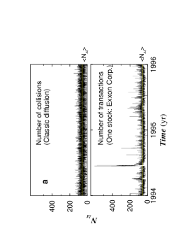
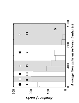
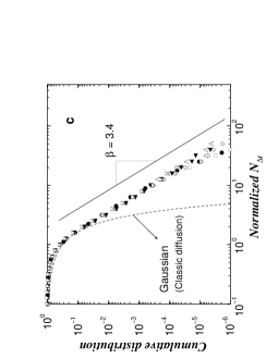
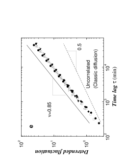
FIG. 1.: Statistical properties of $N_{\Delta t}$. a) The lower panel shows $N_{\Delta t}$ for Exxon Corporation with $\Delta t=30$ min and the average value $\langle N_{\Delta t}\rangle\approx 52$. The upper panel shows a sequence of uncorrelated Gaussian random numbers with the same mean and variance, which depicts the number of collisions in $N_{\Delta t}$ for the classic diffusion problem. Note that in contrast to diffusion, $N_{\Delta t}$ for Exxon shows frequent large events of the magnitude of tens of standard deviations, which would be forbidden for Gaussian statistics. b) The histogram of the average time interval between trades $\langle\delta t\rangle$ for the 1000 stocks studied. In order to ensure that the sampling time interval $\Delta t$ for each stock contains sufficient number of transactions, we partition the stocks into 6 groups (I–VI) based on $\langle\delta t\rangle$. For a specific group, we choose a sampling time $\Delta t$ at least 10 times larger than the average value of $\langle\delta t\rangle$ for that group. We choose the sampling time interval $\Delta t=30,39,65,78,130$ and $190$ min respectively for groups I–VI. c) Log-log plot of the cumulative distribution of $N_{\Delta t}$ for the stocks in each of the six groups in b). Since each stock has a different average value of $\langle N_{\Delta t}\rangle$, we use a normalized number of transactions $n_{\Delta t}\equiv N_{\Delta t}/\langle N_{\Delta t}\rangle$. Each symbol shows the cumulative distribution $P\{n_{\Delta t}>x\}$ of the normalized number of transactions $n_{\Delta t}$ for all stocks in each group. d) The histogram of exponents obtained by fits to the cumulative distributions $P\{N_{\Delta t}>x\}$ for each of the 1000 stocks. For the 1000 stocks studied, we obtain an average value $\beta=3.40$. We calculate an error estimate $\pm 0.05$ by dividing the standard deviation of the estimates of $\beta$ by $\sqrt{1000}$.

e) In order to accurately quantify time correlations in $N_{\Delta t}$, we use the method of detrended fluctuations [36] often used to obtain accurate estimates of power-law correlations. We plot the detrended fluctuations $F(\tau)$ as a function of the time scale $\tau$ on a log-log scale for each of the 6 groups. Absence of long-range correlations would imply $F(\tau)\sim\tau^{0.5}$, whereas $F(\tau)\sim\tau^{\nu}$ with $0.5<\nu\leq 1$ show power-law correlations with long-range persistence. For each group, we plot $F(\tau)$ averaged over all stocks in that group. In order to detect genuine long-range correlations, the U-shaped intraday pattern for $N_{\Delta t}$ has been removed by dividing each $N_{\Delta t}$ by the intraday pattern [14]. For $0.5<\nu<1.0$, correlation function exponent $\nu_{cf}$ and $\nu$ are related through $\nu_{cf}=2-2\nu$. f) The histogram of the exponents $\nu$ obtained by fits to $F(\tau)$ for each of the 1000 stocks shows a relatively narrow spread of $\nu$ around the mean value $\nu=0.85\pm 0.01$.

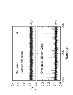
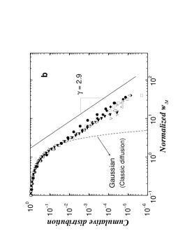
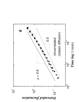
FIG. 2.: Statistical properties of $w_{\Delta t}$. a) The local standard deviation $w_{\Delta t}$ computed from price changes $\delta p_{i}$ due to every transaction in the interval $[t,\,t+\Delta t]$ for Exxon Corporation (lower panel) in contrast to uncorrelated Gaussian random numbers with the same mean value $\langle w_{\Delta t}\rangle\approx 0.08$ and variance (upper panel). The time series of $w_{\Delta t}$ for Exxon shows a number of large events of the size of tens of standard deviations. Intervals having fewer than 4 transactions are not used for computing $w_{\Delta t}$. Note that the large values of $N_{\Delta t}$ in Fig. 1a do not correspond to large values of $w_{\Delta t}$, showing that $N_{\Delta t}$ and $w_{\Delta t}$ are weakly, if at all, correlated. b) Log-log plot of the cumulative distribution of $w_{\Delta t}$ for each of the six groups defined in Fig. 1b. Since the average value $\langle w_{\Delta t}\rangle$ changes from one stock to another, we normalize $w_{\Delta t}$ by $\langle w_{\Delta t}\rangle$. Each symbol shows the cumulative distribution of the normalized $w_{\Delta t}$ for all stocks in each group. c) The power law exponents for the cumulative distribution of $w_{\Delta t}$ obtained by fits to the cumulative distributions of each of the 1000 stocks separately. We obtain an average value $\gamma=2.9\pm 0.1$. d) Log-log plot of the detrended fluctuation $F(\tau)$ as a function of the time lag $\tau$. Each symbol shows $F(\tau)$ averaged over all stocks in each group. e) The histogram of detrended fluctuation exponents obtained by fitting $F(\tau)$ for each stock separately. We obtain an average value $\mu=0.60\pm 0.01$.

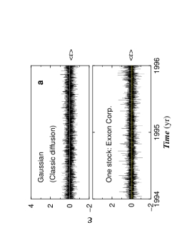
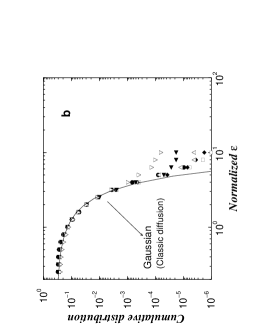
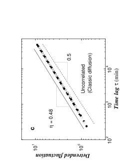
FIG. 3.: Statistical properties of $\epsilon$. a) The time series of $\epsilon\equiv G_{\Delta t}/(w_{\Delta t}\sqrt{N_{\Delta t}})$ for Exxon Corporation (lower panel) in contrast with a sequence of uncorrelated Gaussian random numbers with the same mean and variance which depicts $x_{\Delta t}/(w_{\Delta t}\sqrt{N_{\Delta t}})$ for classic diffusion (upper panel). b) The positive tail of the cumulative distribution of $\epsilon$ for the six groups. We normalize $\epsilon$ by its standard deviation in order to compare different stocks. Each symbol shows the cumulative distributions of the normalized $\epsilon$ for all stocks in each of the six groups. The negative tail (not shown) displays similar behavior. c) Log-log plot of the detrended fluctuation $F(\tau)$ averaged for all stocks belonging to each of the six groups. d) The histogram of detrended fluctuation exponents obtained by fits to $F(\tau)$ for each stock. We obtain the average value $\eta=0.48\pm 0.06$.

REFERENCES

- [1] Bachelier, L., Théorie de la spéculation. Ann. Sci. École Norm. Sup. III-17, 21–86 (1900).
- [2] The Trades and Quotes Database, 24 CD-ROMs for 1994-95, published by the New York Stock Exchange.
- [3] Bouchaud, J.-P. & Potters, M., Theory of Financial Risk (Cambridge University Press, Cambridge 2000)
- [4] Farmer, J. D., Physicists Attempt to Scale the Ivory Towers of Finance. Computing in Science & Engineering 26, November Issue.
- [5] Mandelbrot, B. B., The variation of certain speculative prices. J. Business 36, 394–419 (1963).
- [6] Mantegna, R. N. & Stanley, H. E., Scaling behavior in the dynamics of an economic index. Nature 376, 46–49 (1995).
- [7] Ghashgaie, S., Breymann, W., Peinke, J., Talkner, P., & Dodge, Y., Turbulent cascades in foreign exchange markets. Nature 381, 767–770 (1996).
- [8] Pagan, A., The econometrics of financial markets. J. Empirical Finance 3, 15–102 (1996).
- [9] Lux, T., The stable Paretian hypothesis and the frequency of large returns: An examination of major German stocks. Applied Financial Economics 6, 463-75 (1996).
- [10] Loretan, M. & Phillips, P. C. B., Testing the covariance stationarity of heavy-tailed time series. J. Empirical Finance 1, 211–248 (1994)
- [11] Muller, U. A., Dacorogna, M. M. & Pictet, O. V., Heavy tails in high-frequency financial data. A Practical Guide to Heavy Tails, Adler, R. J., Feldman, R. E. & Taqqu, M. S. (eds.) 283–311 (Birkhäuser Publishers, 1998).
- [12] Plerou, V., Gopikrishnan, P., Amaral, L. A. N., Meyer, M. & Stanley, H. E., Scaling of the distribution of price fluctuations of individual companies. Phys. Rev. E. 60, 6519-6529 (1999).
- [13] Ding, Z., Granger, C. W. J. & Engle, R. F., A long memory property of stock market returns and a new model. J. Empirical Finance 1, 83–105 (1993).
- [14] Liu, Y., Cizeau, P., Meyer, M., Peng, C.-K & Stanley, H. E., Quantification of correlations in economic time series. Physica A 245, 437–440 (1997).
- [15] Lundin, M., Dacorogna, M. M., & Muller, U. A., in Financial Markets Tick by Tick, P. Lequeux (ed.), 91–126, (John Wiley & Sons, 1999).
- [16] Anderson, T., Bollerslev, T., Diebold, F. & Labys, P., The distribution of exchange rate volatility. NBER Working Paper WP6961 (1999).
- [17] Arnoedo, A., Muzy, J.-F. & Sornette, D., Causal cascade in the stock market from the “infrared” to the “ultraviolet”. Eur. Phys. J. B 2, 277–282 (1998).
- [18] Chandrasekhar, S., Stochastic problems in Physics and Astronomy. Rev. Mod. Phys. 15 1–91 (1943), in Selected Papers on Noise and Stochastic Processes, Wax, N. (ed.) (Dover Publications Inc., New York, 1954).
- [19] Montroll, E. W. & Shlesinger, M. F., The wonderful world of random walks, in Nonequilibrium Phenomena II. From Stochastics to Hydrodynamics Lebowitz, J. L. & Montroll, E. W. (eds.) 1-121 (North-Holland, Amsterdam, 1984).
- [20] Bouchaud, J.-P. & Georges, A., Anomalous diffusion in disordered media: statistical mechanisms, models, and physical applications. Phys. Rep. 195, 127 (1990).
- [21] Clark, P. K., A subordinated stochastic process model with finite variance for speculative prices. Econometrica 41, 135–155 (1973).
- [22] Mandelbrot, B. B. & Taylor, H., On the distribution of stock price differences. Operations Research 15, 1057–1062 (1962).
- [23] Epps, T. W. & Epps, M. L., The stochastic dependence of security price changes and transaction volumes: Implications of the mixture-of-distributions hypothesis. Econometrica 44, 305-321 (1976).
- [24] Tauchen, G. & Pitts, M., The price variability-volume relationship on speculative markets. Econometrica 57, 485–505 (1983).
- [25] Stock, J., Estimating continuous time processes subject to time deformation. Journal of the American Statistical Association 83 77–85 (1988).
- [26] Guillaume, D. M., Pictet, O. V., Muller, U. A. & Dacorogna, M. M., Unveiling non-linearities through time scale transformations. Olsen group preprint OVP.1994-06-26 (1995), available at http://www.olsen.ch.
- [27] Feller, W., An Introduction to Probability Theory and its Applications (John Wiley, New York, 1966).
- [28] Engle, R. F., (ed.) ARCH: Selected Readings (Oxford University Press, Oxford, 1995).
- [29] Ghysels, E., Harvey, A. & Renault, E., Stochastic Volatility. Handbook of Statistics Vol. 14, Statistical Methods in Finance, G. S. Maddala (ed.), 119–191 (North-Holland, Amsterdam, 1996).
- [30] Jones, C., Gautam, K. & Lipson, M., Transactions, volumes and volatility. Reviews of Financial Studies 7, 631–651 (1994).
- [31] Ane, T. & Geman, H., Order flow, transaction clock and normality of asset returns. Journal of Finance, forthcoming (2000).
- [32] Lux, T. & Marchesi, M., Scaling and criticality in a stochastic multi-agent model of a financial market. Nature 397, 498–500 (1999).
- [33] Cont, R. & Bouchaud, J.-P., Herd behavior and aggregate fluctuations in financial markets. Macroeconomic Dynamics, forthcoming; preprint cond-mat/9712318.
- [34] Bouchaud, J.-P. & Cont, R., A Langevin approach to stock market fluctuations and crashes. Eur. Phys. J. B 6, 543–550 (1998).
- [35] Easley, D. & O’Hara, M., Time and the process of security price adjustment. Journal of Finance 47, 905–927.
- [36] Peng, C.-K., et. al., Mosaic organization of DNA nucleotides. Phys. Rev. E 49, 1685–1689 (1994).