Exact ground states for a class of one-dimensional frustrated quantum spin models

Abstract

We have found the exact ground state for two frustrated quantum spin-1/2 models on a linear chain. The first model describes ferromagnet – antiferromagnet transition point. The singlet state at this point has double-spiral ordering. The second model is equivalent to special case of the spin-1/2 ladder. It has non-degenerate singlet ground state with exponentially decaying spin correlations and there is an energy gap. The exact ground state wave function of these models is presented in a special recurrent form and recurrence technics of expectation value calculations is developed.

I Introduction

Last decade frustrated Heisenberg models have been a subject of intensive studies^1-12. Of main interests are ground state properties with respect to variations of exchange integrals and character of the phase transitions. In particular, these properties may be important in the theory of high-$T_{c}$ superconductivity.

There is much interest in quantum spin systems with competing interactions for which exact ground state can be constructed. The first example of such a model has been given by Majumdar and Ghosh¹³. They have considered $s=\frac{1}{2}$ chain with antiferromagnetic nearest- and next-nearest neighbor interactions and the strength of the second interaction is one half of the first. The ground state of this model is two-fold degenerate, consists of dimerized singlets and there is a gap in the spectrum of excited states.

Another example found by Affleck, Kennedy, Lieb and Tasaki¹⁴ is an $S=1$ spin chain with special bilinear and biquadratic interactions (AKLT model). This model has unique resonating-valence-bond ground state and ground state correlations have exponential decay. Besides, there is the gap between ground state and excited states. Further generalizations of the AKLT model have been studied in a number recent papers¹⁵.

In this paper we present two classes of $s=\frac{1}{2}$ chains for which exact ground state wave function has a special recurrent form. These models have competing ferro- and antiferromagnetic interactions and their ground states can be either ferromagnetic or singlet depending on the relation between exchange integrals. The first type of exactly solvable models is related to the systems at the ferromagnet-antiferromagnet transition point when the ferromagnetic and the singlet states are degenerate. The calculation of the spin correlation function in the singlet ground state shows the spiral magnetic order at this point.

The model of the second type has the nearest, next-nearest and next-next-nearest neighbor interactions depending on one parameter. This model has the non-degenerate singlet ground state for cyclic chains and for a certain region of the parameter and its ground state properties are similar to that of AKLT model. In other words, this model has all properties of the ”Haldane scenario”¹⁶, though it is the model with half-integer spin. We note, however, that the considered model has two sites in an unit cell and it is equivalent to the special case of a spin ladder. In some limit this model reduces to the effective spin-1 chain for which the ground state wave function coincides with that for the AKLT model.

The paper is organized as follows. In Section 2 we will consider the model of the first type and describe the exact singlet ground state wave function as well as details of the spin correlation function calculations. Section 3 and Appendix present the study of the model of the second type. The results of the paper will be summarized in Section 4.

II Frustrated spin chain at ferromagnet-antiferromagnet transition points.

A The exact ground state wave function.

Let us consider $s=\frac{1}{2}$ spin model with nearest- and next-nearest neighbor interactions given by the Hamiltonian

$$H=-\sum_{i=1}^{M}({\bf S}_{2i-1}\cdot{\bf S}_{2i}-\frac{1}{4})+J_{23}\sum_{i=1}^{M}({\bf S}_{2i}\cdot{\bf S}_{2i+1}-\frac{1}{4})+J_{13}\sum_{i=1}^{N}({\bf S}_{i}\cdot{\bf S}_{i+2}-\frac{1}{4}),$$ (1)

with periodic boundary conditions and even $N=2M$.

If $J_{23}<1$, then the ground state of (1) is ferromagnetic (singlet) at $\delta<0$ ($\delta>0$), where $\delta=J_{13}+\frac{J_{23}}{2(1-J_{23})}$ (Fig.1). The equation $\delta=0$ defines the line of transition points from the ferromagnetic to the singlet state, when energies of these states are zero. The model (1) along this line is given by the Hamiltonian depending on the parameter $\nu$ ($\nu>0$):

\begin{picture}(11.0,8.0)\centerline{\hbox{\psfig{angle=0,width=256.0748pt}}} \end{picture}

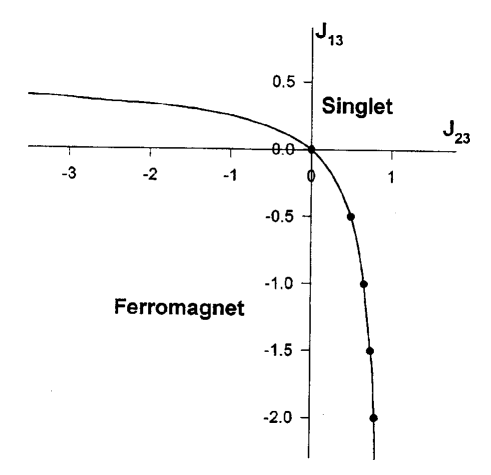
FIG. 1.: $T=0$ phase diagram of the model (1). The solid line is the boundary between the ferromagnetic and singlet phases. Model (1) along this line is given by Hamiltonian (2). Circles correspond to the special cases of this Hamiltonian.

$$H=-\sum_{i=1}^{M}({\bf S}_{2i-1}\cdot{\bf S}_{2i}-\frac{1}{4})-(\nu-1)\sum_{i=1}^{M}({\bf S}_{2i}\cdot{\bf S}_{2i+1}-\frac{1}{4})+\frac{\nu-1}{2\nu}\sum_{i=1}^{N}({\bf S}_{i}\cdot{\bf S}_{i+2}-\frac{1}{4}),$$ (2)

with periodic boundary conditions.

We note that the Hamiltonian (2) has a symmetry: its spectrum coincides with the spectrum of $\widetilde{H}(\nu)$ obtained by the following transformation

$\displaystyle\widetilde{H}(\nu)=(\nu-1)~{}H(\frac{\nu}{\nu-1}),\qquad\nu>1$

This transformation permutes the factors at the first and the second terms in the Hamiltonian (2). Thus, due to the symmetry it is sufficient to consider the range $0\leq\nu\leq 2$.

First, we will show that the ground state energy of (2) is zero. Let us represent the Hamiltonian (2) as a sum of Hamiltonians $H_{n}$ of cells containing three sites

$$H=\sum_{i=1}^{M}(H_{2i-1}+H_{2i}),$$ (3)

where

$\displaystyle H_{2i-1}=-\frac{1}{2}({\bf S}_{2i-1}\cdot{\bf S}_{2i}-\frac{1}{4})-\frac{\nu-1}{2}({\bf S}_{2i}\cdot{\bf S}_{2i+1}-\frac{1}{4})+\frac{\nu-1}{2\nu}({\bf S}_{2i-1}\cdot{\bf S}_{2i+1}-\frac{1}{4}),$

$\displaystyle H_{2i}=-\frac{1}{2}({\bf S}_{2i+1}\cdot{\bf S}_{2i+2}-\frac{1}{4})-\frac{\nu-1}{2}({\bf S}_{2i}\cdot{\bf S}_{2i+1}-\frac{1}{4})+\frac{\nu-1}{2\nu}({\bf S}_{2i}\cdot{\bf S}_{2i+2}-\frac{1}{4})$

Eigenvalues of each $H_{n}$ are

$\displaystyle\lambda_{1}=\lambda_{2}=0,\qquad\lambda_{3}=\frac{\nu^{2}-\nu+1}{2\nu}>0$

We will present a singlet wave function which is the exact one of each $H_{n}$ with zero energy and, therefore, it is the exact ground state wave function of (2). This function has a form

$$\Psi_{0}(M)=P_{0}\Psi_{M},$$ (4)

where

$$\Psi_{M} = (s_{1}^{+}+\nu s_{2}^{+}+\nu s_{3}^{+}\ldots+\nu s_{N}^{+})(s_{3}^{+}+\nu s_{4}^{+}\ldots+\nu s_{N}^{+})\ldots$$ (6)

$$\times(s_{2n-1}^{+}+\nu s_{2n}^{+}\ldots+\nu s_{N}^{+})\ldots(s_{N-1}^{+}+\nu s_{N}^{+})\mid 1,2,\ldots N\rangle,$$

where $s_{i}^{+}$ is the $s=\frac{1}{2}$ raising operator.

Eq.(5) contains $M=\frac{N}{2}$ operator multipliers and the vacuum state $\mid 1,2,\ldots N\rangle$ is the state with all spins pointing down. The function $\Psi_{M}$ is the eigenfunction of $S_{z}$ with $S_{z}=0$ but it is not the eigenfunction of ${\bf S}^{2}$. $P_{0}$ is a projector onto the singlet state. This operator is¹⁷

$\displaystyle P_{0}=\frac{1}{8\pi^{2}}\int_{0}^{2\pi}d\alpha\int_{0}^{2\pi}d\beta\int_{0}^{\pi}\sin\gamma d\gamma~{}e^{i\alpha\stackrel{{\scriptstyle\wedge}}{{S_{z}}}}e^{i\gamma\stackrel{{\scriptstyle\wedge}}{{S_{x}}}}e^{i\beta\stackrel{{\scriptstyle\wedge}}{{S_{z}}}},$

where $\stackrel{{\scriptstyle\wedge}}{{S}}_{x(z)}$ are components of the total spin operator.

The function $\Psi_{M}$ contains components with all possible values of spin $S$ ($0\leq S\leq M$) and, in fact, a fraction of the singlet is exponentially small at large $N$. This component is filtered out by the operator $P_{0}$.

It is not difficult to check that

$$H_{n}\Psi_{M}=0$$ (7)

for $n=1,\ldots(N-2)$ and, therefore, the ground state energies for all values of spin $S$ of an open chain describing by the Hamiltonian

$$H_{\rm op}=\sum_{n=1}^{N-2}H_{n}$$ (8)

are zero.

The operators $H_{N-1}$ and $H_{N}$ do not give zero acting on $\Psi_{M}$ but

$$H_{N-1(N)}P_{0}\Psi_{M}=P_{0}H_{N-1(N)}\Psi_{M}=0$$ (9)

The latter equation can be easily checked using the fact the first bracket in (5) can be replaced by $(1-\nu)s_{1}^{+}$ under the projector $P_{0}$.

Eqs.(6) and (8) mean that $\Psi_{0}(M)$ is the exact singlet ground state wave function of (2) for any $M$ and the ground state energy is zero. We note that the ground state energy coincides with its exact lower bound because $H$ is the sum of non-negative defined operators (Eq.(3)). Of course, the trivial ferromagnetic state has zero energy as well.

In particular case, $\nu=2$, when $J_{12}=J_{23}=-1$ and $J_{13}=\frac{1}{4}$, another form of the exact singlet ground state wave function has been found in Ref.18. It reads

$\displaystyle\Psi=\sum[i,j][k,l][m,n]\ldots,$

where $[i,j]$ denotes the singlet pair and the summation is made for any combination of spin sites under the condition that $i<j,k<l,m<n\ldots$. However, it is not clear how this function can be generalized to $\nu\neq 2$.

The following general statements relevant to the Hamiltonian (2) can be proved:

1). The ground states of open chains described by (7) in the sector with fixed total spin $S$ are non-degenerate and their energies are zero.

2). For cyclic chains the ground state in the $S=0$ sector is non-degenerate and has momentum $\pi$. The ground state energies for $0<S<M$ are non-zero.

3). The singlet ground state wave function for open and cyclic chains coincide with each other.

4). The singlet ground state wave function $\Psi_{0}(M)$ is superstable¹⁹ with respect to any cell operator $H_{n}$, i.e. $\Psi_{0}(M)$ is the ground state wave function of the Hamiltonian $H+\lambda H_{n}$ for $-1<\lambda<\infty$.

B The norm of the ground state wave function.

Let us return to the problem of the projection of the function $\Psi_{M}.$ As one can see from Eq.(5) the function $\Psi_{M}$ satisfies a recurrent equation

$$\Psi_{M}=\left[(s_{1}^{+}+\nu s_{2}^{+})+\nu S^{+}(N-2)\right]\mid 1,2\rangle\Psi_{M-1},$$ (10)

where $\Psi_{M-1}$ is the function (5) for the system of $(N-2)$ spins on sites $3,4,\ldots N$ and $S^{+}(N-l)=\sum_{i=l+1}^{N}\,s_{i}^{+}.$

In principle, it is possible to generate $\Psi_{0}(M)$ starting from $M=1$ and using Eqs.(4) and (9). However, it is more convenient to obtain the recurrent formulae for expectation values (norm and correlators) with respect to the function $\Psi_{0}(M)$ directly.

First, we consider a norm of $\Psi_{0}(M)$ which has a form

$$G_{M}=\langle\Psi_{0}(M)\Psi_{0}(M)\rangle=\langle\Psi_{M}P_{0}\Psi_{M}\rangle=\frac{1}{2}\int_{0}^{\pi}\Phi_{M}(\gamma)\sin\gamma d\gamma,$$ (11)

where

$\displaystyle\Phi_{M}(\gamma)=\Phi_{M}(\gamma_{1},\gamma_{2})\mid_{\gamma_{1}=\gamma_{2}=\gamma}$

and

$$\Phi_{M}(\gamma_{1},\gamma_{2})=\langle\Psi_{M}\exp(i\frac{\gamma_{1}}{2}S^{+}(N)+i\frac{\gamma_{2}}{2}S^{-}(N))\Psi_{M}\rangle$$ (12)

Commuting operators in Eq.(11) and using the fact, that $S_{z}\Psi_{M}=0,$ we rewrite Eq.(11) in a form

$$\Phi_{M}(\gamma_{1},\gamma_{2})=\langle\Psi_{M}\exp(izS^{-}(N))\exp(iz^{\prime}S^{+}(N))\Psi_{M}\rangle,$$ (13)

where

$\displaystyle z=\sqrt{\frac{\gamma_{2}}{\gamma_{1}}}\tan\frac{\sqrt{\gamma_{1}\gamma_{2}}}{2},\qquad z^{\prime}=\sqrt{\frac{\gamma_{1}}{\gamma_{2}}}\frac{\sin\sqrt{\gamma_{1}\gamma_{2}}}{2}$

It follows from Eqs.(9) and (12) that the function $\Phi_{M}(\gamma_{1},\gamma_{2})$ satisfies the equation

$$\Phi_{M}(\gamma_{1},\gamma_{2}) = [1+\nu^{2}-(1+\nu)^{2}zz^{\prime}+\nu(\nu+1)(1-zz^{\prime})(z\frac{\partial}{\partial z}+z^{\prime}\frac{\partial}{\partial z^{\prime}})$$

$$-\nu^{2}(1-zz^{\prime})^{2}\frac{\partial^{2}}{\partial z\partial z^{\prime}}]~{}\Phi_{M-1}(\gamma_{1},\gamma_{2})$$

Using this equation we obtain for $\Phi_{M}(\gamma)$

$$\Phi_{M}(\gamma) = [1+\nu^{2}-(1+\nu)^{2}\sin^{2}\frac{\gamma}{2}+\nu(\nu+1)\sin\gamma\frac{d}{d\gamma}$$ (15)

$$-\nu^{2}\cos^{2}\frac{\gamma}{2}(\frac{d^{2}}{d\gamma^{2}}+\frac{1}{\sin\gamma}\frac{d}{d\gamma})]\Phi_{M-1}(\gamma)$$

The solution of Eq.(13) is

$$\Phi_{M}(y)=L^{M}(y)\Phi_{0}(y),$$ (16)

where

$$L(y)=\frac{(1-\nu)^{2}}{2}+\frac{(1+\nu)^{2}}{2}y-\nu(\nu+1)(1-y^{2})\frac{d}{dy}-\frac{\nu^{2}}{2}(1+y)^{2}\frac{d}{dy}(1-y)\frac{d}{dy},$$ (17)

$y=\cos\gamma$ and $\Phi_{0}(y)=1.$

According to Eq.(15) $\Phi_{M}(y)$ is a polynomial in $y$ of order $M$. It turns out that further calculations will be simplified if $\Phi_{M}(y)$ is expanded over Legendre polynomials $P_{n}(y)$ :

$$\Phi_{M}(y)=\sum_{n=0}^{M}c_{n}(M)P_{n}(y)$$ (18)

The coefficients $c_{n}(l)$ are defined by the recurrent equation

$$c_{n}(l+1)=\frac{n}{2n-1}\frac{(\nu n+1)^{2}}{2}c_{n-1}(l)+\frac{\nu^{2}(n^{2}+n)+(\nu-1)^{2}}{2}c_{n}(l)+\frac{n+1}{2n+3}\frac{(\nu n+\nu-1)^{2}}{2}c_{n+1}(l)$$ (19)

with initial condition $c_{0}(0)=1.$ Besides, $c_{n}(l)=0$ at $n>l.$

The norm $G_{M}$ is given by

$$G_{M}=\frac{1}{2}\int_{-1}^{1}\Phi_{M}(y)dy=c_{0}(M)$$ (20)

C Spin correlations.

The spin correlation functions can be found in the same way as $G_{M}.$ It is convenient to express the scalar product ${\bf S}_{i}\cdot{\bf S}_{j}$ by the permutation operator $p_{ij}=2{\bf S}_{i}\cdot{\bf S}_{j}+\frac{1}{2}$. Then the non-normalized expectation value $Q(i,j)=$ $\langle\Psi_{0}(M)({\bf S}_{i}\cdot{\bf S}_{j}-\frac{1}{4})\Psi_{0}(M)\rangle$ is

$$Q(i,j)=-\frac{1}{4}\langle\Psi_{0}(M)(p_{i,j}-1)^{2}\Psi_{0}(M)\rangle=-\frac{1}{4}\langle\Psi_{M}(p_{i,j}-1)P_{0}(p_{i,j}-1)\Psi_{M}\rangle$$ (21)

The equations for $Q(i,j)$ can be obtained as in the derivation of Eqs.(14)-(15). They are somewhat different for even and odd $i$. For example, the equations for $Q(1,n)$ have forms

$$Q(1,2l)=-\frac{(\nu-1)^{2}}{4}\int_{-1}^{1}\frac{1+y}{2}(L^{l-2}L_{1}L^{M-l}~{}1)dy,$$ (22)

$$Q(1,2l-1)=-\frac{\nu^{2}(\nu-1)^{2}}{4}\int_{-1}^{1}\frac{1+y}{2}(L^{l-2}L_{2}L^{M-l}~{}1)dy,$$ (23)

where

$\displaystyle L_{1}=1-2\nu(1-y)\frac{d}{dy}-\nu^{2}(1+y)\frac{d}{dy}(1-y)\frac{d}{dy},$

$\displaystyle L_{2}=1-2(1-y)\frac{d}{dy}-(1+y)\frac{d}{dy}(1-y)\frac{d}{dy}$

It is clear, that

$\displaystyle Q(2,n+2)=Q(1,N-n+1)$

Making use consequent integration of Eqs.(20) and (21), we obtain

$$\int_{-1}^{1}\frac{1+y}{2}(L^{l-2}L_{1(2)}L^{M-l}1)dy=\int_{-1}^{1}\frac{1+y}{2}(\widetilde{L}^{l-2}1)(L_{1(2)}L^{M-l}1)dy=\int_{-1}^{1}(\widetilde{L}_{1(2)}\widetilde{L}^{l-2}1)(L^{M-l}1)dy,$$

where

$\displaystyle\widetilde{L}=\widetilde{L}_{1}=\frac{1}{2}+\frac{(2\nu-1)^{2}}{2}y-\nu(2\nu-1)(1-y^{2})\frac{d}{dy}-\frac{\nu^{2}}{2}(1+y)^{2}\frac{d}{dy}(1-y)\frac{d}{dy},$

$\displaystyle\widetilde{L}_{2}=\frac{1+y}{2}-(1-y^{2})\frac{d}{dy}-\frac{(1+y)^{2}}{2}\frac{d}{dy}(1-y)\frac{d}{dy},$

So, Eqs.(20) and (21) can be rewritten as

$$Q(1,2l)=-\frac{(\nu-1)^{2}}{4}\int_{-1}^{1}\widetilde{\Phi}_{l-1}(y)~{}\Phi_{M-l}(y)dy,$$ (24)

$$Q(1,2l-1)=-\frac{\nu^{2}(\nu-1)^{2}}{4}\int_{-1}^{1}(\widetilde{L}_{2}\widetilde{\Phi}_{l-2}(y))~{}\Phi_{M-l}(y)dy,$$ (25)

where

$$\widetilde{\Phi}_{l}(y)=\widetilde{L}^{l}(y)~{}1$$ (26)

The function $\widetilde{\Phi}_{l}(y)$ can be expanded over Legendre polynomials similarly to $\Phi_{l}(y)$

$$\widetilde{\Phi}_{l}(y)=\sum_{n=0}^{l}a_{n}(l)P_{n}(y),$$ (27)

and coefficients $a_{n}(l)$ satisfy the equations

$$a_{n}(l+1)=\frac{n}{2n-1}\frac{(\nu n+\nu-1)^{2}}{2}a_{n-1}(l)+\frac{\nu^{2}(n^{2}+n)+1}{2}a_{n}(l)+\frac{n+1}{2n+3}\frac{(\nu n+1)^{2}}{2}a_{n+1}(l)$$ (28)

with initial condition $a_{0}(0)=1$ and $a_{n}(l)=0$ at $n>l.$

Using Eqs.(18), (22) and (23) we can express the correlation function $K(1,n)=\langle{\bf S}_{1}\cdot{\bf S}_{n}\rangle/G_{M}$ in the forms

$$K(1,2l)=\frac{1}{4}-\frac{(\nu-1)^{2}}{2c_{0}(M)}\sum_{n=0}^{l-1}\frac{a_{n}(l-1)c_{n}(M-l)}{2n+1},$$ (29)

$$K(1,2l-1)=\frac{1}{4}-\frac{\nu^{2}(\nu-1)^{2}}{2c_{0}(M)}\sum_{n=0}^{l-1}\frac{b_{n}(l-1)c_{n}(M-l)}{2n+1},$$ (30)

where coefficients $b_{n}(l-1)$ are defined by $a_{n}(l-2)$ as follows:

$$b_{n}(l-1)=\frac{1}{2}\frac{n^{3}}{2n-1}a_{n-1}(l-2)+\frac{n^{2}+n+1}{2}a_{n}(l-2)+\frac{1}{2}\frac{(n+1)^{3}}{2n+3}a_{n+1}(l-2)$$ (31)

Therefore, the calculation of the spin correlation function reduces to the solution of the recurrent equations (17) and (26) which were used for numerical calculations of the spin correlation function for finite systems.

At large $M$ the solutions of the recurrent equations (17) and (26) have scaling forms:

$$c_{n}(M)=2M(M!)^{2}\nu^{2M}s\exp\left(Mf_{0}(s)+\frac{2-\nu}{\nu}\ln M+f_{1}(s)\right),$$ (32)

$$a_{n}(M)=2M(M!)^{2}\nu^{2M}s\exp\left(Mf_{0}(s)-\frac{2-\nu}{\nu}\ln M+g_{1}(s)\right),$$ (33)

where the parameter

$\displaystyle s=\frac{2n+1}{2M}$

can be considered as a continuous variable.

We note that Eqs.(30) and (31) are not valid for special values of $\nu$, $\nu=\frac{1}{m+1}$ ($m=0,1,2\ldots$). For these $\nu$ the last term in (17) vanishes when $n=m$ and Eq.(17) reduces to ($m+1$) equations for $c_{n}(l)$ with $n\leq m$.

The recurrent equations (17) and (26) at $M>>1$ and $\nu\neq\frac{1}{m+1}$ reduce to differential ones for $f_{0}(s)$, $f_{1}(s)$ and $g_{1}(s).$ For example, $f_{0}(s)$ satisfies the equation

$\displaystyle\exp\left(f_{0}(s)-s\frac{df_{0}(s)}{ds}\right)=s^{2}\cosh^{2}\left(\frac{1}{2}\frac{df_{0}(s)}{ds}\right)$

with initial condition $f_{0}(1)=-\ln 4$.

Its implicit solution is

$$f_{0}(s)=-2\ln\xi+2\frac{\sin\xi}{\xi}\ln\tan\frac{\xi}{2},$$ (34)

where

$\displaystyle s=\frac{\sin\xi}{\xi}$

As it follows from Eq.(32), $a_{n}(M)$ and $c_{n}(M)$ as a functions of $n$ have a sharp maximum at $\frac{n}{M}=\frac{2}{\pi}.$

The functions $f_{1}(s)$ and $g_{1}(s)$ are given by

$$f_{1}(s)=-\frac{2+\nu}{\nu}\ln\xi+\frac{4-\nu}{2\nu}\ln\sin\xi-\frac{1}{2}\ln(\frac{\sin\xi}{\xi^{2}}-\frac{\cos\xi}{\xi})+C\frac{\nu-1}{\nu^{2}},$$ (35)

$$g_{1}(s)=\frac{2-3\nu}{\nu}\ln\xi+\frac{3\nu-4}{2\nu}\ln\sin\xi-\frac{1}{2}\ln(\frac{\sin\xi}{\xi^{2}}-\frac{\cos\xi}{\xi})+C\frac{\nu-1}{\nu^{2}},$$ (36)

where constant $C\simeq 0.969$.

To obtain $K(1,2l)$ at $N\rightarrow\infty$ we substitute Eqs.(30)-(34) into Eq.(27) and replace the sum over $n$ by the integral over $s.$ This integral is calculated by the method of steepest descent. The saddle point is $s_{0}=\frac{1}{\pi}\sin(\frac{2\pi l}{N})$ and the integrand does not depend on parameter $\nu$. The final result for the spin correlation function $K(1,2l)$ at $N\rightarrow\infty$ is also independent on $\nu$:

$$K(1,2l)=\frac{1}{4}\cos\left(\frac{2\pi(2l-1)}{N}\right)+O\left(\frac{1}{N}\right)$$ (37)

For the particular case $\nu=2$ Eq.(35) has been obtained earlier in Ref.18.

The corresponding calculations for $K(1,2l-1)$ to within terms $\sim\frac{1}{N}$ lead to the same expression (35). But taking into account terms $\sim\frac{1}{N}$ we find that the difference $K(1,2l-1)-K(1,2l)$ is

$\displaystyle K(1,2l-1)-K(1,2l)=\frac{\pi}{N}\frac{\nu-1}{\nu}\sin\left(\frac{4\pi l}{N}\right)+O\left(\frac{1}{N^{2}}\right)$

The latter equation means that the double-spiral structure exists. The pitch angle of each spiral is $\frac{4\pi}{N}$ and there is a small shift angle $\triangle\varphi=\frac{2\pi}{N}\frac{2-\nu}{\nu}$ between them:

$$K(1,2l)=\frac{1}{4}\cos\left(\frac{2\pi(2l-1)}{N}-\triangle\varphi\right),$$ (38)

$$K(1,2l+1)=\frac{1}{4}\cos\left(\frac{4\pi l}{N}\right)$$ (39)

This shift angle reflects the fact that the unit cell contains two sites unless $\nu=2$.

Eqs.(36) and (37) show that the long range spiral order exists in the singlet ground state of the Hamiltonian (2) in the thermodynamic limit and the double-spiral state is formed.

It is interesting to note that correlators (36) and (37) coincide with those obtained by using the simple ‘quasi-classical’ trial wave function in a form

$\displaystyle\psi_{cl}=\exp\left(\sum_{n=1}^{N}\varsigma_{n}s_{n}^{+}\right)\left|1,2,\ldots N\right\rangle,$

where

$\displaystyle\varsigma_{n}=\exp\left(\frac{2\pi n}{N}+\frac{(-1)^{n}\pi}{N}\frac{\nu-2}{\nu}\right)$

Thus, the quantum ground state of the large-$N$ limit resembles the classical one though for small size systems the quantum fluctuations are essential.

The formation of the spirals having the period which is equal to the system size reflects the tendency to the creation of the incommensurate spiral state at the antiferromagnetic region when $\delta>0$. The behavior of the system in the vicinity of the transition point has been studied by us⁷ for the model (1) with $J_{12}=J_{23}=-1$, $J_{13}=\frac{1}{4}+\delta$. For $\delta\ll 1$ the period of the spiral is finite and is proportional to $\delta^{-\frac{1}{2}}$. The transition from the ferromagnetic to the singlet state is a phase transition of the second order with respect to $\delta$.

D Special cases of the model.

There are the special points, $\nu=\frac{1}{m}$ ($m=1,2,\ldots$) at which Eqs.(36) and (37) are not valid.

At $\nu=\frac{1}{2}$ the function (4) reduces to the product of singlets

$$\Psi_{0}(M)=[2,3][4,5]\ldots[N,1],$$ (40)

and $K(2,3)=K(4,5)=\ldots=K(N,1)=-\frac{3}{4}$. Other spin correlators are zero.

Analysis of Eqs.(17), (26) and (27) shows that the ground state correlations of the model (2) with $\nu=\frac{1}{m}$ ($m\geq 3$) have antiferromagnetic character with an exponentially decay:

$\displaystyle K(1,n+1)\sim(-1)^{n}\exp(-\frac{n}{r_{c}}),$

where the correlation length is

$$r_{c}=-2\ln^{-1}\left(1-\frac{2}{m(m-1)}\right)$$ (41)

The crossover between the spiral state at $\frac{1}{m}<\nu<\frac{1}{m-1}$ and the antiferromagnetic state at $\nu=\frac{1}{m}$ occurs in the exponentially small (at $N\gg 1$) vicinity of these spacial points. At $m\gg 1$

$$r_{c}=m^{2},$$ (42)

and the correlation length diverges when $\nu$ trends to zero along the special points and there is the Neel ordering in this limit.

At $\nu=1$, when $J_{12}=-1$, $J_{23}=J_{13}=0$, the system is divided into the ferromagnetic pairs $1-2,3-4,\ldots$.

Using the second order perturbation theory with respect to $(\nu-1)$, we reduce the model (2) at $\nu\rightarrow 1$ to the effective spin-$1$ Hamiltonian

$$H_{eff} = \frac{(\nu-1)^{2}}{8}\sum_{n=1}^{M}\left\{-({\bf L}_{n}\cdot{\bf L}_{n+1}-1)+{\bf L}_{n}\cdot{\bf L}_{n+2}\right.$$ (44)

$$\left.-\frac{1}{2}({\bf L}_{n}\cdot{\bf L}_{n+1})({\bf L}_{n+1}\cdot{\bf L}_{n+2})-\frac{1}{2}({\bf L}_{n+1}\cdot{\bf L}_{n+2})({\bf L}_{n}\cdot{\bf L}_{n+1})\right\},$$

with $M$ spins $L=1$.

The exact singlet ground state wave function of the Hamiltonian (41) can be obtained from the Eqs.(4) and (5). It has a form

$$\Psi_{0}(M)=P_{0}~{}L_{1}^{+}(L_{2}^{+}+L_{3}^{+}+...+L_{M}^{+})\ldots(L_{M-1}^{+}+L_{M}^{+})L_{M}^{+}~{}|-1,\ldots,-1\rangle,$$ (45)

where $L_{i}^{+}$ are raising operators of spin $1$.

The ground state correlation function of (41) $K(1,n+1)=\langle{\bf L}_{1}\cdot{\bf L}_{n+1}\rangle/G_{M}$ is found from Eqs.(36) and (37). It is

$\displaystyle K(1,n+1)=\cos\left(\frac{2\pi n}{M}\right)$

Finally, we note that it is possible to calculate higher terms of the perturbation theory and to obtain an effective spin-$1$ Hamiltonians which are proportional to the third, fourth and higher power of the small parameter $(\nu-1)$. All of them have zero ground state energy as well as (41).

III Frustrated spin chain with an antiferromagnetic ground state.

A The model and its exact ground state.

In the preceding section the spin model at the ferromagnet-antiferromagnet transition point has been studied. The exact singlet ground state wave function at this point is given by Eq.(4). In this section the function (4) will be generalized to give the exact ground state wave function of new special one-dimensional frustrated spin-$\frac{1}{2}$ model. This model has the unique singlet ground state (for the cyclic chain) with an exponentially decay of correlations and there is a gap to the excitations.

Let us consider the wave function which depends on two parameters and has the form (4)

$$\Psi_{0}(M)=P_{0}\Psi_{M},$$ (46)

where

$$\Psi_{M} = (s_{1}^{+}+\nu_{1}s_{2}^{+}+\nu_{2}s_{3}^{+}\ldots+\nu_{2}s_{N}^{+})(s_{3}^{+}+\nu_{1}s_{4}^{+}+\nu_{2}s_{5}^{+}\ldots+\nu_{2}s_{N}^{+})\ldots$$ (48)

$$\times(s_{N-1}^{+}+\nu_{1}s_{N}^{+})~{}\left|1,2,\ldots N\right\rangle$$

We will construct the Hamiltonian for which $\Psi_{0}(M)$ is the exact ground state wave function as the sum of the local four-sites Hamiltonians

$$H=H_{1,2,3,4}+H_{3,4,5,6}+\ldots+H_{N-3,N-2,N-1,N}+H_{N-1,N,1,2}$$ (49)

The Hamiltonians $H_{i,i+1,i+2,i+3}$ are chosen in the form:

$$H_{i,i+1,i+2,i+3} = J_{12}\left[({\bf S}_{i}\cdot{\bf S}_{i+1}-\frac{1}{4})+({\bf S}_{i+2}\cdot{\bf S}_{i+3}-\frac{1}{4})\right]$$ (52)

$$+2J_{13}\left[({\bf S}_{i}\cdot{\bf S}_{i+2}-\frac{1}{4})+({\bf S}_{i+1}\cdot{\bf S}_{i+3}-\frac{1}{4})\right]$$

$$+2J_{23}({\bf S}_{i+1}\cdot{\bf S}_{i+2}-\frac{1}{4})+2J_{14}({\bf S}_{i}\cdot{\bf S}_{i+3}-\frac{1}{4})$$

Thus, the model has nearest ($J_{12}$ and $J_{23}$), next-nearest ($J_{13}$) and next-next-nearest ($J_{14}$) neighbor interactions. In fact, this model is equivalent to the spin-$\frac{1}{2}$ ladder with different interactions as it is shown in Fig.2.

\begin{picture}(11.0,4.0)\centerline{\hbox{\psfig{angle=0,width=256.0748pt}}} \end{picture}

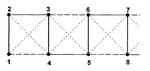
FIG. 2.: Spin ladder representation of the model (45). Different lines correspond to different exchange interactions.

We demand that $\Psi_{0}(M)$ is the eigenfunction of each local Hamiltonian with the eigenvalue $\varepsilon<0$, i.e.

$$H_{i,i+1,i+2,i+3}\Psi_{0}(M)=\varepsilon~{}\Psi_{0}(M)$$ (53)

The exchange integrals $J_{ij}$ and the energy $\varepsilon$ is defined by the Schrödinger equation:

$$H_{1,2,3,4}\Psi_{M}=\varepsilon~{}\Psi_{M}$$ (54)

Let us represent the function $\Psi_{M}$ in the form

$$\Psi_{M}=\left[\widehat{q}_{1}+\nu_{2}\widehat{q}_{2}S^{+}(N-4)+\nu_{2}^{2}S^{+2}(N-4)\right]\left|1,2,3,4\right\rangle\Psi_{M-2},$$ (55)

where

$\displaystyle\widehat{q}_{1}=s_{1}^{+}s_{3}^{+}+\nu_{1}(s_{1}^{+}s_{4}^{+}+s_{2}^{+}s_{3}^{+})+\nu_{1}^{2}s_{2}^{+}s_{4}^{+}+\nu_{2}(1+\nu_{1})s_{3}^{+}s_{4}^{+},$

$\displaystyle\widehat{q}_{2}=s_{1}^{+}+\nu_{1}s_{2}^{+}+(1+\nu_{2})s_{3}^{+}+(\nu_{1}+\nu_{2})s_{4}^{+}$

The equation

$$H_{1,2,3,4}\widehat{q}_{1}\left|1,2,3,4\right\rangle=\varepsilon~{}\widehat{q}_{1}\left|1,2,3,4\right\rangle$$ (56)

reduces to five equations for four exchange integrals and the energy $\varepsilon$. The necessary condition of the existence of a solution with $\varepsilon<0$ is

$$1+\nu_{1}+\nu_{2}=0$$ (57)

So, under this condition there is only one parameter of the Hamiltonian (45). It is convenient to take the value $\mu=\frac{2+\nu_{1}}{2\nu_{1}+1}$ as a system parameter. Then, the solution of Eq.(50) at $\nu_{1}=\frac{2-\mu}{2\mu-1}$ and $\nu_{2}=\frac{\mu+1}{1-2\mu}$ yields the following expressions for $J_{ij}$ and $\varepsilon$:

$$\begin{array}[]{c}J_{12}=\frac{(1-2\mu)(2-\mu)}{9},\qquad J_{23}=-\frac{1}{3}\frac{(2-\mu)^{2}(\mu-1)\mu}{(\mu+1)^{2}}\\ \\ J_{13}=\frac{(2\mu-1)(2-\mu)(\mu-1)^{2}}{6(\mu+1)^{2}},\qquad J_{14}=\frac{(2\mu-1)^{2}(\mu-1)}{3(\mu+1)^{2}}\\ \\ \varepsilon=-\frac{3\mu(\mu-1)^{2}}{(\mu+1)^{2}}\end{array}$$ (58)

It turns out that the equation

$\displaystyle H_{1,2,3,4}\widehat{q}_{2}\left|1,2,3,4\right\rangle=\varepsilon~{}\widehat{q}_{2}\left|1,2,3,4\right\rangle$

with $J_{ij}$ and $\varepsilon$ given by Eq.(52) is satisfied automatically.

As it will be proven in Appendix the function $\Psi_{M}$ with $\nu_{1}=-\nu_{2}-1$ contains the singlet and the triplet components only, i.e.

$$S^{+2}(N)\Psi_{M}=0$$ (59)

Therefore, the last term in Eq.(49) vanishes and $\Psi_{M}$ is the eigenfunction of $H_{1,2,3,4}$ with the eigenvalue $\varepsilon$.

Generally, the Hamiltonian $H_{1,2,3,4}$ has following eigenstates: one quintet, three triplets and two singlets. Two of them (one singlet and one triplet) have the energy $\varepsilon$ while other four states have higher energies at $\mu>0$ ($\mu\neq 1$). At $\mu<0$ the ground state of $H_{1,2,3,4}$ is a quintet with zero energy. In Appendix we will show that the wave function $\Psi_{M}$ is the eigenfunction with the eigenvalue $\varepsilon$ of each local Hamiltonian $H_{i,i+1,i+2,i+3}$ excluding that for $i=N-1$. Therefore, the ground state energy of the open chain at $\mu>0$ is $(\frac{N}{2}-1)\varepsilon$ and it coincides with the exact lower bound of the energy similarly to the model of Section 2. However, in the contrast with the latter the present model is four-fold degenerate for the open chain.

As for the Hamiltonian $H_{N-1,N,1,2}$ the function $\Psi_{M}$ is not its eigenfunction, but

$\displaystyle H_{N-1,N,1,2}\Psi_{0}(M)=\varepsilon~{}\Psi_{0}(M)$

(see Appendix) and

$\displaystyle H\Psi_{0}(M)=\frac{N}{2}\varepsilon~{}\Psi_{0}(M)$

As it follows from Eq.(52) the spectrum of $H(\mu)$ coincides with the spectrum of $\widetilde{H}(\mu)$ which is connected with $H(\mu)$ by transformation

$\displaystyle\widetilde{H}(\mu)=\mu^{2}H(\frac{1}{\mu})$

This transformation permutes the factors at the third and the last terms in Eq.(46). Therefore, it is sufficient to consider the Hamiltonian $H(\mu)$ in the region $-1\leq\mu\leq 1$.

The ground state of $H$ is ferromagnetic at $\mu<0$. When $0<\mu<1$ the ground state of the cyclic chain is the non-degenerate singlet. The point $\mu=0$ is the ferromagnet-antiferromagnet transition point. At this point the present model coincides with the model (2) at the special point $\nu=\frac{1}{3}$. As it follows from Eq.(52) this transition is the phase transition of the first order with respect to $\mu$.

At $\mu=\frac{1}{2}$ the only non-zero exchange integral is $J_{23}$ and the ground state consists of non-interacting singlet pairs $2-3,4-5,\ldots,1-N$. When $\mu\rightarrow 1$ the first term in Eq.(46) dominates and the system is divided into weekly interacting ferromagnetic pairs $1-2,3-4,\ldots$ . Using the second order perturbation theory with respect to the small parameter $(\mu-1)$ we reduce the Hamiltonian $H$ (Eq.45) to the effective spin-$1$ model given by

$\displaystyle H=\frac{(\mu-1)^{2}}{16}H_{eff},$

where

$$H_{eff}=\sum_{n=1}^{M}\left\{5{\bf L}_{n}\cdot{\bf L}_{n+1}+{\bf L}_{n}\cdot{\bf L}_{n+2}+\frac{1}{2}({\bf L}_{n}\cdot{\bf L}_{n+1}-{\bf L}_{n+1}\cdot{\bf L}_{n+2})^{2}-6\right\},$$ (60)

and ${\bf L}_{n}$ is spin-$1$ operator.

The ground state wave function of (54) can be obtained from Eq.(43) at $\mu=1$. It reads

$$\Psi_{0}(M)=P_{0}~{}({\bf L}_{1}^{+}-2{\bf L}_{2}^{+}-\ldots-2{\bf L}_{M}^{+})({\bf L}_{2}^{+}-2{\bf L}_{3}^{+}-\ldots-2{\bf L}_{M}^{+})\ldots\times({\bf L}_{M-1}^{+}-2{\bf L}_{M}^{+}){\bf L}_{M}^{+}~{}\left|-1,-1,\ldots-1\right\rangle$$ (61)

It is remarkable that the function (55) coincides with the ground state wave function of the AKLT model. Therefore, the ground state physics of the model given by Eq.(54) and AKLT one is the same, though the Hamiltonians of these two models are different.

B Spin correlations in the ground state.

First, we calculate the norm of the ground state wave function. It is convenient to express the function $\Psi_{M}$ in terms of the parameter $\mu$ and to introduce a new function $\widetilde{\Psi}_{M}$

$\displaystyle\Psi_{M}=(2\mu-1)^{-M}~{}\widetilde{\Psi}_{M},$

where

$$\widetilde{\Psi}_{M} = \left[(2\mu-1)s_{1}^{+}+(2-\mu)s_{2}^{+}-(\mu+1)S^{+}(N-2)\right]\left[(2\mu-1)s_{3}^{+}+(2-\mu)s_{4}^{+}-(\mu+1)S^{+}(N-4)\right]$$

$$\ldots\left[(2\mu-1)s_{N-1}^{+}+(2-\mu)s_{N}^{+}\right]\left|1,2,\ldots N\right\rangle$$

According to Eq. (18) the norm of $\widetilde{\Psi}_{0}(M)=P_{0}\widetilde{\Psi}_{M}$ is

$\displaystyle G_{M}=\left\langle\widetilde{\Psi}_{0}(M)\widetilde{\Psi}_{0}(M)\right\rangle=\frac{1}{2}\int_{-1}^{1}\Phi_{M}(y)dy$

For the present model the function $\Phi_{l}(y)$ is defined by the equation

$$\Phi_{l}(y)=L^{l}(y)~{}1,$$ (62)

where

$\displaystyle L(y)=\frac{9(1-\mu)^{2}}{2}+\frac{(1+\mu)^{2}}{2}\left[y+2(1-y^{2})\frac{d}{dy}-(1+y)^{2}\frac{d}{dy}(1-y)\frac{d}{dy}\right]$

The solution of Eq.(56) is

$\displaystyle\Phi_{l}(y)=\frac{\omega_{1}^{l}+3\omega_{2}^{l}}{4}+\frac{\omega_{1}^{l}-\omega_{2}^{l}}{4}y,$

where

$\displaystyle\omega_{1}=6(\mu^{2}-\mu+1),\qquad\omega_{2}=2(\mu-2)(2\mu-1)$

This form of $\Phi_{l}(y)$ reflects the fact that the function $\widetilde{\Psi}_{M}$ contains the singlet and the triplet components only. Thus, $G_{M}$ is

$$G_{M}=\frac{\omega_{1}^{M}+3\omega_{2}^{M}}{4}$$ (63)

As $\left|\frac{\omega_{2}}{\omega_{1}}\right|<1$ then $G_{M}=\frac{1}{4}\omega_{1}^{M}$ at $M\rightarrow\infty$.

The spin correlation functions can be found in the similar way as in the Section 2. In analogy with the Eqs.(19)-(20), we obtain

$$Q(N-2l-1,N)=-\frac{1}{8}\int_{-1}^{1}(L^{M-l-1}\Phi_{l+1}^{\prime}(y))dy,$$ (64)

where

$\displaystyle\Phi_{l+1}^{\prime}(y)=\langle\widetilde{\Psi}_{l+1}(p_{N-2l-1,N}-1)P_{0}(p_{N-2l-1,N}-1)\widetilde{\Psi}_{l+1}\rangle$

Carrying out the necessary calculations, we find

$$\Phi_{l+1}^{\prime}(y)=4(\mu+1)^{2}(2-\mu)^{2}\omega_{1}^{l-1}+\omega_{2}^{l+1}+(2\mu-1)^{2}\left[(2\mu^{2}-2\mu+5)\omega_{1}^{l-1}+(2\mu^{2}+10\mu-1)\omega_{2}^{l-1}\right](1+y)$$

Substituting $\Phi_{l+1}^{\prime}(y)$ into Eq.(58) we obtain for the spin correlation function $K(1,2l+2)=K(N-2l-1,N)$

$$K(1,2)=\frac{1}{4}-\frac{9(\mu-1)^{2}}{2\omega_{1}}\frac{1+3\left(\frac{\omega_{2}}{\omega_{1}}\right)^{M-1}}{1+3\left(\frac{\omega_{2}}{\omega_{1}}\right)^{M}},$$ (65)

$$K(1,2l+2)=-\frac{3(\mu+1)^{2}}{\omega_{1}\omega_{2}}\frac{(2\mu-1)^{2}\left(\frac{\omega_{2}}{\omega_{1}}\right)^{l}+(\mu-2)^{2}\left(\frac{\omega_{2}}{\omega_{1}}\right)^{M-l}}{1+3\left(\frac{\omega_{2}}{\omega_{1}}\right)^{M}},$$ (66)

where $l=1,2,\ldots M-1$.

The similar calculations for $K(1,2l+1)$ result in

$$K(1,2l+1)=\frac{3(\mu+1)^{2}}{2\omega_{1}}\frac{\left(\frac{\omega_{2}}{\omega_{1}}\right)^{l}+\left(\frac{\omega_{2}}{\omega_{1}}\right)^{M-l}}{1+3\left(\frac{\omega_{2}}{\omega_{1}}\right)^{M}}$$ (67)

The correlators $K(2,n)$ have been obtained by using the symmetry of the system (see Fig.2). For example,

$\displaystyle K(2,3)=K(1,N),\quad etc.$

In the thermodynamic limit $M\rightarrow\infty$ and $l\ll M$ Eqs.(59)-(61) reduce to

$$K(1,2)=-\frac{3}{4}\frac{\omega_{2}}{\omega_{1}},$$ (68)

$$K(1,2l+2)=-\frac{3(\mu+1)^{2}(2\mu-1)^{2}}{\omega_{1}\omega_{2}}\left(\frac{\omega_{2}}{\omega_{1}}\right)^{l}$$ (69)

$$K(1,2l+1)=\frac{3(\mu+1)^{2}}{2\omega_{1}}\left(\frac{\omega_{2}}{\omega_{1}}\right)^{l}$$ (70)

The correlators have the exponential decay and the correlation length $r_{c}$ is

$$r_{c}(\mu)=2\ln^{-1}\left|\frac{\omega_{1}(\mu)}{\omega_{2}(\mu)}\right|$$ (71)

It follows from Eq.(65) that the ground state has ultrashort-range correlations. For example, $r_{c}(0)=2\log^{-1}\left(\frac{3}{2}\right)$ (this value coincides with $r_{c}$ given by Eq.(39) with $m=3$) and $r_{c}(1)=2\log^{-1}3$. In the latter case $r_{c}$ coincides with correlation length of the AKLT model. At $\mu=\frac{1}{2}$ the only non-zero correlators are $K(2,3)=K(4,5)=\ldots=K(N,1)=-\frac{3}{4}$ in accordance with the dimer character of the ground state.

The value $\omega_{2}(\mu)$ changes the sign at $\mu=\frac{1}{2}$ and as it follows from Eqs.(62), (63) and (64) the correlators show the antiferromagnetic structure of the ground state at $0\leq\mu\leq\frac{1}{2}$ while at $\frac{1}{2}\leq\mu\leq 1$ there are ferromagnetic correlations inside pairs $(1,2),(3,4),\ldots$ and the antiferromagnetic correlations between the pairs.

C Energy gap.

The Hamiltonian $H$ of the cyclic chain has a singlet-triplet gap $\Delta$ for finite $N$. It is evident that for $\mu=\frac{1}{2}$ the gap exists for $N\rightarrow\infty$ and $\Delta(\frac{1}{2})=\frac{1}{6}$. The existence of the finite gap at the thermodynamic limit in the range $0<\mu<1$ follows from the continuity of the function $\Delta(\mu)$. It is also clear that $\Delta(\mu)$ at $N\rightarrow\infty$ vanishes at the boundary points $\mu=0$ and $\mu=1$ when the ground state is degenerate and there are low-lying spin wave excitations.

Unfortunately, the method of the exact calculation of $\Delta(\mu)$ in the thermodynamic limit is unknown. For $\mu\simeq\frac{1}{2}$ the gap can be found by using the perturbation theory in $(\mu-\frac{1}{2})$. In this case $\Delta(\mu)$ is

$$\begin{array}[]{c}\Delta(\mu)=\frac{1}{6}+O((\mu-\frac{1}{2})^{2}),\quad\mu\leq\frac{1}{2}\\ \\ \Delta(\mu)=\frac{1}{6}-\frac{8}{9}(\mu-\frac{1}{2})+O((\mu-\frac{1}{2})^{2}),\quad\mu\geq\frac{1}{2}\end{array}$$ (72)

Eq.(66) shows that $\Delta(\mu)$ has a cusp at $\mu=\frac{1}{2}$. For the approximate calculation $\Delta(\mu)$ we use the trial function of the triplet state in the form

$$\Psi_{t}=\sum_{n=1}^{N}c_{n}s_{n}^{+}\Psi_{0}(M),$$ (73)

where

$\displaystyle c_{2l-1}=ae^{ikl},\quad c_{2l}=be^{ikl},\quad k=\frac{4\pi}{N}t,\quad t=1,\ldots M$

This trial function gives $\Delta(\mu)$ which is

$$\Delta(\mu)=\frac{2\sum_{n\neq m}c_{n}^{*}c_{m}K(n,m)J_{n,m}-2\sum_{n\neq m}|c_{n}^{2}|K(n,m)J_{n,m}}{\frac{3}{4}\sum_{n}|c_{n}^{2}|+\sum_{n\neq m}c_{n}^{*}c_{m}K(n,m)}$$ (74)

Function (68) has minima at $k=\frac{4\pi}{N}$ and $k=\pi$ for $0<\mu<\frac{1}{2}$ and $\frac{1}{2}<\mu<1$, respectively. Then $\Delta(\mu)$ at $N\rightarrow\infty$ is

$$\begin{array}[]{c}\Delta(\mu)=\frac{8}{3}\frac{(\mu+1)^{4}(\mu-1)^{2}}{\omega_{1}(\omega_{1}+\omega_{2})},\qquad 0<\mu<\frac{1}{2}\\ \\ \Delta(\mu)=\frac{2}{3}(1+\frac{\omega_{2}}{\omega_{1}})(\mu-1)^{2},\qquad\frac{1}{2}<\mu<1\end{array}$$ (75)

The dependance of $\Delta(\mu)$ given by Eq.(69) is shown on Fig.3 together with the results of extrapolations of exact finite-chain calculations. Both dependences agree very well for $\mu\geq\frac{1}{2}$. In particular, Eq.(69) correctly reproduces (66) at $\mu\simeq\frac{1}{2}$. However, $\Delta(\mu)$ given by Eq.(69) is not zero at $\mu=0$ while numerical calculations fit the dependence $\Delta(\mu)\sim\sqrt{\mu}$ at $\mu\rightarrow 0$.

\begin{picture}(11.0,8.0)\centerline{\hbox{\psfig{angle=0,width=256.0748pt}}} \end{picture}

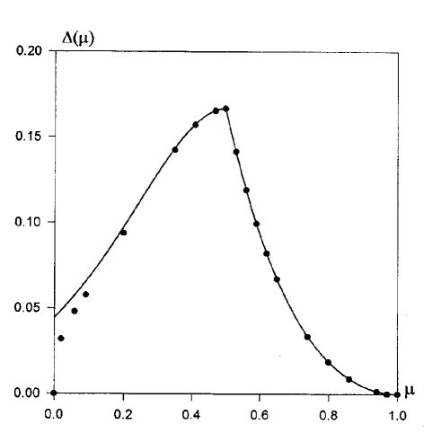
FIG. 3.: Singlet-triplet gap of the model (45) as a function of the parameter $\mu$. The circles denote the results of the extrapolation of an exact finite-chain calculations. The solid line represents the dependence $\Delta(\mu)$ given by Eq.(69).

We note that the trial function of the type (67) gives the value $0.7407$ for the singlet-triplet gap in the AKLT model. This estimate is close to the value $0.7143$ obtained by another approach in Ref.20.

The above consideration refers to the gap in the cyclic chain. The open chain has four-fold degenerate ground state. Finite chain calculations show that the spin of the lowest excitation is $S=2$ . However, there are also two excited singlet and triplet states the energies of which are close to that of $S=2$. The difference of these three eigenvalues decreases to zero exponentially at $N\rightarrow\infty$. We expect that these states are degenerate in the thermodynamic limit (at $\mu=\frac{1}{2}$ they are degenerate for finite $N$). The gap in the open chain equals to the difference between the energies of the degenerate ground state and the lowest excited one. The extrapolation of the results of finite-chain calculations to $N\rightarrow\infty$ gives the finite gap in the open chains at $0<\mu<1$. Its value is very close to that for the cyclic chains.

IV Summary

We have studied a class of the one dimensional quantum spin-$\frac{1}{2}$ models with competing interactions. The exact ground state wave function of these models is found in the special recurrent form. The Hamiltonians of these models are the sums of local, non-commuting with each other Hamiltonians; the ground state wave function of the total Hamiltonian is the ground state solution for each of them. This means that this ground state wave function is superstable¹⁹ with respect to each local Hamiltonian.

One of the studied models describes the transition point from the ferromagnetic to the spiral state when the energies of these two states are equal to each other. It is interesting to compare the exact quantum singlet state with the classical one. Both states are the states of a helical type (excluding some special cases) and their spin correlation functions are identical in the thermodynamic limit though quantum effects are essential for finite chains. This fact is rather surprising for the one-dimensional model with spin $\frac{1}{2}$.

Another exactly solvable Hamiltonian has the antiferromagnetic ground state. This state is non-degenerate for the closed chains and is four-fold degenerate for the open ones. The Hamiltonian depends on the one parameter $\mu$ and there are two special values, $\mu=0$ and $\mu=1$ where the singlet and the ferromagnetic states are degenerate. The value $\mu=0$ is the ferromagnet-antiferromagnet transition point where the phase transition of the first order with respect to $\mu$ occurs.

The ground state is characterized by the exponential decay of correlators with a very short correlation length, and there is the gap in the excitation spectrum at $0<\mu<1$. Thus, this model has all properties suggested by Haldane¹⁶ for the one-dimensional Heisenberg antiferromagnet with integer spin. The first model for which all these properties have been proved rigorously is the AKLT model. Our model is the one with spin $\frac{1}{2}$. Affleck and Lieb²¹ have shown for the translationally invariant and the isotropic Heisenberg Hamiltonians that for half-integer spin chain either the excitation spectrum is gapless or the ground state is degenerate. The existence of the finite gap in our model does not contradict to Affleck-Lieb theorem because this model is not translationally invariant. It has two sites in the unit cell and is equivalent to the special ladder model. Moreover, in the limit $\mu\rightarrow 1$ its ground state wave function reduces to that for the AKLT model.

V Acknowledgments

We are grateful to Profs.M.Ya.Ovchinnikova and V.N.Prigodin for helpful discussions. This work was supported by ISTC under Grant No.015-94 and in part by RFFR No.33727.

VI Appendix

We prove that square of the total raising operator annihilates $\Psi_{M}$ if the condition (51) is satisfied. The recurrent equation for $S^{+2}(N)\Psi_{M}$ is

$$\begin{array}[]{c}S^{+2}(N)\Psi_{M}=2(1+\nu_{1}+\nu_{2})s_{1}^{+}s_{2}^{+}|1,2\rangle~{}S^{+}(N-2)\Psi_{M-1}+\\ \\ +\left[(1+2\nu_{2})s_{1}^{+}+(\nu_{1}+2\nu_{2})s_{2}^{+}+\nu_{2}S^{+}(N-2)\right]|1,2\rangle~{}S^{+2}(N-2)\Psi_{M-1}\end{array}$$ (76)

The first term in Eq.(A1) vanishes under the condition (51) and, therefore,

$$S^{+2}(N)\Psi_{M}=\left[(1+2\nu_{2})s_{1}^{+}+(\nu_{1}+2\nu_{2})s_{2}^{+}+\nu_{2}S^{+}(N-2)\right]$$

$$\times\left[(1+2\nu_{2})s_{3}^{+}+(\nu_{1}+2\nu_{2})s_{4}^{+}+\nu_{2}S^{+}(N-4)\right]\ldots\times(s_{N-1}^{+}+s_{N}^{+})^{2}\left[s_{N-1}^{+}+\nu_{1}s_{N}^{+}\right]|1,2,\ldots N\rangle=0$$

This equation means that the wave function $\Psi_{M}$ contains the singlet and triplet components only.

Now we prove that $\widetilde{\Psi}_{0}(M)$ is the eigenfunction of each local Hamiltonian in (45). Of course, consequentely the same will be true for $\Psi_{0}(M)$.

The function $\widetilde{\Psi}_{M}$ satisfies the recurrent equation

$$\widetilde{\Psi}_{M}=\left(\widehat{u}_{12}\widetilde{\Psi}_{M-1}-(\mu+1)S^{+}(N-2)\widetilde{\Psi}_{M-1}\right)|1,2\rangle,$$ (77)

where

$\displaystyle\widehat{u}_{12}=(2\mu-1)s_{1}^{+}+(2-\mu)s_{2}^{+}$

Let us consider functions $\varphi_{M}^{+}=S^{+}(N)\widetilde{\Psi}_{M}$, $\varphi_{M}^{-}=S^{-}(N)\widetilde{\Psi}_{M}$ and $\chi_{M}=S^{-}(N)S^{+}(N)\widetilde{\Psi}_{M}$. The recurrent equations for these functions are obtained from (A2) using (A1). They are

$$\varphi_{M}^{+}=\left((\mu+1)s_{1}^{+}s_{2}^{+}\widetilde{\Psi}_{M-1}+\widehat{v}_{12}\varphi_{M-1}^{+}\right)|1,2\rangle,$$ (78)

$$\varphi_{M}^{-}=\left((\mu+1)(\widetilde{\Psi}_{M-1}-\chi_{M-1})+\widehat{u}_{12}\varphi_{M-1}^{-}\right)|1,2\rangle,$$ (79)

$$\chi_{M}=\left[(\widehat{u}_{12}-\widehat{v}_{12})\widetilde{\Psi}_{M-1}+\widehat{v}_{12}\chi_{M-1}+(\mu+1)(s_{1}^{+}s_{2}^{+}\varphi_{M-1}^{-}-\varphi_{M-1}^{+})\right]|1,2\rangle,$$ (80)

where

$\displaystyle\widehat{v}_{12}=-(2-\mu)s_{1}^{+}-(2\mu-1)s_{2}^{+}$

Eqs.(A2)-(A3) can be written in a matrix form

$$R(M)=D_{12}R(M-1),$$ (81)

where $R(M)$ and $D_{12}$ are $(2\times 2)$ matrices

$\displaystyle R(M)=\left(\begin{array}[]{cc}\widetilde{\Psi}_{M}-\chi_{M}&\varphi_{M}^{+}\\ -\varphi_{M}^{-}&\widetilde{\Psi}_{M}\end{array}\right),$

$\displaystyle D_{12}=\left(\begin{array}[]{cc}\widehat{v}_{12}&(\mu+1)s_{1}^{+}s_{2}^{+}\\ -(\mu+1)&\widehat{u}_{12}\end{array}\right)|1,2\rangle$

Therefore, $R(M)$ is

$$R(M)=D_{12}D_{34}\ldots D_{N-1,N}$$ (82)

As $\widetilde{\Psi}_{M}$ contains the singlet and triplet components only, the projection of $\widetilde{\Psi}_{M}$ onto the singlet is

$$\widetilde{\Psi}_{0}(M)=P_{0}\widetilde{\Psi}_{M}=2\widetilde{\Psi}_{M}-\chi_{M}$$ (83)

It follows from Eqs.(A5)-(A6) that

$$\widetilde{\Psi}_{0}(M)=Tr(D_{12}D_{34}\ldots D_{N-1,N})$$ (84)

This form of $\widetilde{\Psi}_{0}(M)$ is similar to the matrix product wave function of the AKLT model and its generalizations which has been found in Ref.15. Each of four matrix elements of $R(M)$ is the eigenfunction of the local Hamiltonian $H_{i,i+1,i+2,i+3}$ for $i=1,3,\ldots N-3$ because of matrix elements of the product $D_{i,i+1}D_{i+1,i+2}$ are the eigenfunctions of this Hamiltonian. Besides, it can be proved¹⁵ that the four matrix elements of $R(M)$ are the only ground states of (45) and, therefore, the ground state of the open chain is four-fold degenerate.

It is easily to check¹⁵ that the triplet wave functions $R_{12}(M)$ and $R_{21}(M)$ are not eigenfunctions of $H_{N-1,N,1,2}$. On the other hand, using cyclic permutations of matrices under the $trace$, we have

$\displaystyle H_{N-1,N,1,2}\widetilde{\Psi}_{0}(M)=\varepsilon~{}\widetilde{\Psi}_{0}(M)$

and, therefore, the ground state of the cyclic chain is the non-degenerate singlet.

REFERENCES

- [1] E.Dagotto, Int. J. Mod. Phys.B 5, 907 (1991).
- [2] P.Sen and B.K.Chakrabarti, Int.J.Mod.Phys.B 6, 2439 (1992).
- [3] T.Tonegawa and I.Harada, J.Phys.Soc.Japan 56, 2153 (1987).
- [4] A.V.Chubukov and T.Jolicoeur, Phys.Rev.B 44, 12050 (1991).
- [5] A.V.Chubukov. Phys.Rev.B 44, 4693 (1991).
- [6] D.J.J.Farnell and J.B.Parkinson, J.Phys.Condens.Matter 6, 5521 (1994); R.Bursill, G.A.Gehring, D.J.J.Farnell, J.B.Parkinson, Tao Xiang and Chen Zeng, J.Phys.: Condens.Matter. 7, 8605 (1995).
- [7] V.Ya.Krivnov and A.A.Ovchinnikov, Phys.Rev.B 53, 6435 (1996).
- [8] K.Nomura and K.Okamoto, Phys.Lett.A 169, 433 (1992).
- [9] P.M. van den Broek. Phys.Lett.A 77, 261 (1980).
- [10] H.P.Bader and R.Schilling. Phys.Rev.B 19, 3556 (1979).
- [11] C.E.I.Carneiro, M.J.de Oliveira and W.F.Wreszinski, J.Stat.Phys. 79, 347 (1995).
- [12] S.R.White and I.Affleck, Phys.Rev.B 54, 9862 (1996).
- [13] C.K.Majumdar and D.K.Ghosh. J.Math.Phys. 10, 1388, 1399 (1969).
- [14] I.Affleck, T.Kennedy, E.H.Lieb and H.Tasaki. Phys.Rev.Lett. 59, 799 (1987), Commun.Math.Phys. 115, 477 (1988).
- [15] A.Klumper, A.Schadschneider and J.Zittartz, Z.Phys. B 87 , 281 (1992); Europhys. Lett., 24 (4), 293 (1993); C.Lange, A.Klumper and J.Zittartz. Z.Phys. B 96, 267 (1994).
- [16] F.D.M.Haldane. Phys.Lett.A 93, 464 (1983); Phys.Rev.Lett. 50, 1153 (1983).
- [17] P.van Leuven. Physica 45, 86 (1969).
- [18] T.Hamada, J.Kane, S.Nakagawa and Y.Natsume. J.Phys.Soc.Jpn. 57, 1891 (1988); 58, 3869 (1989).
- [19] B.Sutherland and S.Shastry, J.Stat.Phys. 33, 477 (1983).
- [20] S.Knabe, J.Stat.Phys. 52, 627 (1988).
- [21] I.Affleck and E.H.Lieb, Lett.Math.Phys. 12, 57 (1986).