Quantum effects on the BKT phase transition of two-dimensional Josephson arrays

Abstract

The phase diagram of two dimensional Josephson arrays is studied by means of the mapping to the quantum XY model. The quantum effects onto the thermodynamics of the system can be evaluated with quantitative accuracy by a semiclassical method, the pure-quantum self-consistent harmonic approximation, and those of dissipation can be included in the same framework by the Caldeira-Leggett model. Within this scheme, the critical temperature of the superconductor-to-insulator transition, which is a Berezinskii-Kosterlitz-Thouless one, can be calculated in an extremely easy way as a function of the quantum coupling and of the dissipation mechanism. Previous quantum Monte Carlo results for the same model appear to be rather inaccurate, while the comparison with experimental data leads to conclude that the commonly assumed model is not suitable to describe in detail the real system.

Two-dimensional Josephson junction arrays (JJA) [1, 2, 3] have been recently described by means of the two-dimensional quantum XY model. These arrays are made by superconducting islands, where the charge carriers (Cooper pairs) interact with each other through the Coulomb interaction and move between nearest-neighbor islands through the Josephson tunneling mechanism. The following action turns out to describe the system [4, 5]

$$S[\boldsymbol{\phi}] = \int_{0}^{\hbar\beta}\!\!du\bigg{\{}\frac{\hbar^{2}}{2}\sum_{\boldsymbol{ij}}\frac{C_{\boldsymbol{ij}}}{q^{2}}~{}{\dot{\phi}_{\boldsymbol{i}}(u)\,\dot{\phi}_{\boldsymbol{j}}(u)}$$ (1)

$$~{}~{}~{}~{}~{}~{}~{}+J\sum_{\langle{\boldsymbol{ij}}\rangle}\Big{[}1-\cos\big{(}(\phi_{\boldsymbol{i}}(u)-\phi_{\boldsymbol{j}}(u)\big{)}\Big{]}\bigg{\}}~{};$$

it is a variant of the well-known quantum XY model and therefore a Berezinskii-Kosterlitz-Thouless (BKT) transition is expected to occur at some finite temperature: its value is affected by quantum effects, whose importance depends on the relative weight of the two terms in the action. The first one represents the Coulomb interaction between Cooper pairs with charge $q=2e$ and with the capacitance matrix

$$C_{\boldsymbol{ij}}=C_{0}\,\Big{[}\,\delta_{\boldsymbol{ij}}+\eta\,\big{(}z\,\delta_{\boldsymbol{ij}}-{\sum}_{\boldsymbol{d}}\delta_{\boldsymbol{i},\boldsymbol{j+d}}\big{)}\Big{]}~{},$$ (2)

where $C_{0}$ and $C_{1}\equiv{\eta\,C_{0}}$ are the self- and mutual capacitances of the islands, and $\boldsymbol{d}$ runs over the vector displacements of the $z$ nearest-neighbors. The second term describes the Josephson interaction with coupling $J$ between nearest-neighbor islands $\langle{\boldsymbol{ij}}\rangle$, being $\phi_{\boldsymbol{i}}-\phi_{\boldsymbol{j}}$ the phase difference between the $\boldsymbol{i}$th and the $\boldsymbol{j}$th superconducting island. ¿From a quantum mechanical point of view the superconducting phase operators $\hat{\phi_{\boldsymbol{i}}}$ are canonically conjugated to the Cooper-pair number operators $\hat{n}_{\boldsymbol{i}}$, $[\hat{\phi}_{\boldsymbol{i}},\hat{n}_{\boldsymbol{j}}]=i\,\delta_{\boldsymbol{ij}}$. [6]

The phase diagram of square and triangular lattices of Josephson Junctions was experimentally [7] investigated and compared with the results of quantum Monte Carlo (QMC) simulations [3] of the above model.

In this paper we present an analytical study of the phase diagram of JJA based on the effective potential approach, or pure-quantum self-consistent harmonic approximation [8] (PQSCHA), where the effect of quantum dissipation is also considered. In mesoscopic systems, like JJA, environmental effects can modify the physical properties of the isolated system. In order to study the open system, an additional term to the action (1) is thus inserted [9, 10]:

$$S_{\rm D}[\boldsymbol{\phi}]=\frac{1}{2}\int_{0}^{\hbar\beta}\!\!\!\!du\int_{0}^{\hbar\beta}\!\!\!\!du^{\prime}\sum_{\boldsymbol{ij}}K_{\boldsymbol{ij}}(u{-}u^{\prime})~{}\phi_{\boldsymbol{i}}(u)\,\phi_{\boldsymbol{j}}(u^{\prime})~{},$$ (3)

where the kernel matrix ${\boldsymbol{K}}(u)=\{K_{\boldsymbol{ij}}(u)\}$ is a real symmetric matrix and, as a function of $u$, is even and periodic, ${\boldsymbol{K}}(u)={\boldsymbol{K}}(-u)={\boldsymbol{K}}(\beta{-}u)$, and satisfies $\int_{0}^{\beta}{du}\,{\boldsymbol{K}}(u)=0$. It contains the whole information about the environmental coupling, in particular it is related to the classical damping memory functions $\gamma_{\boldsymbol{ij}}(t)$ by

$$K_{n,{\boldsymbol{ij}}}=|\nu_{n}|{\hat{\gamma}}_{\boldsymbol{ij}}(|\nu_{n}|)~{},$$ (4)

where $\nu_{n}=2\pi{n}/\hbar\beta$ are the Matsubara frequencies, $\hat{\gamma}_{\boldsymbol{ij}}(s)$ means the Laplace transform of $\gamma_{\boldsymbol{ij}}(t)$, and

$${\boldsymbol{K}}_{n}=\int_{0}^{\hbar\beta}du~{}{\boldsymbol{K}}(u)~{}\cos\nu_{n}u$$ (5)

is the $n$th Matsubara component of the kernel matrix.

In Eq. (1), the Coulomb term is like a kinetic energy contribution (with $\boldsymbol{C}/q^{2}$ as the mass matrix), while the Josephson term plays the role of the potential energy. For large capacitive coupling the classical limit is approached and the system behaves as a classical XY model, displaying a BKT phase transition [11] at the classical critical temperature. In the opposite limit, the energy cost for transferring charges between neighboring islands is high, so the charges tend to be localized and phase ordering tends to be suppressed at lower temperatures. An important role in this system is played by the Coulomb interaction range, that can be quantified by means of the parameter $\eta$, i.e. the ratio between the mutual- and the self-capacitance of the junctions. The connection between $\eta$ and the charging interaction range can be found observing that the latter is proportional to the inverse of the capacitance matrix [5]. The Josephson coupling of an island with its neighbors, $Jz$, defines the overall energy scale for the system, while the characteristic quantum energy scale $\hbar\Omega$ can be identified considering the bare dispersion relation,

$$\hbar^{2}\Omega_{\boldsymbol{k}}^{2}=\frac{q^{2}J}{C_{0}}~{}\frac{z\,\mu_{\boldsymbol{k}}}{1+z\,\eta\,\mu_{\boldsymbol{k}}}~{},$$ (6)

where $\mu_{\boldsymbol{k}}=1{-}\frac{1}{z}\sum_{\boldsymbol{d}}\cos(\boldsymbol{k{\cdot}d})$, and choosing $\Omega$ as the maximum frequency

$$\Omega^{2}\equiv\max\left\{\Omega_{\boldsymbol{k}}^{2}\right\}=\frac{q^{2}J}{\hbar^{2}C_{0}}\cdot\begin{cases}\displaystyle{\frac{8}{1+8\,\eta}}&\square~{}\text{lattice}~{},\\ \displaystyle{\frac{9}{1+9\,\eta}}&\triangle~{}\text{lattice}~{}.\end{cases}$$ (7)

One can define a meaningful quantum coupling parameter, which rules the importance of ‘quanticity’ in the system, as the ratio between the two energy scales

$$g=\frac{\hbar\Omega}{z\,J}~{}.$$ (8)

The thermodynamic properties of the system are studied here by means of the PQSCHA, which was recently extended to treat quantum open systems [12]. By means of this approximation scheme the thermodynamics of the quantum system (1) with dissipation (3) can be reduced to an effective classical problem, where the pure-quantum part of the fluctuations is taken into account at the self-consistent harmonic level through a temperature-dependent renormalization coefficient, while nonlinear thermal fluctuations and quantum harmonic excitations are fully accounted for. Following the prescription of Ref. [12] the PQSCHA effective potential for our system reads

$$V_{\rm eff}=J_{\rm eff}\sum_{\langle{\boldsymbol{ij}}\rangle}\big{[}1-\cos(\phi_{\boldsymbol{i}}-\phi_{\boldsymbol{j}})\,\big{]}~{},$$ (9)

where we do not consider some additive uniform terms, since they do influence neither thermal averages nor the critical behavior. The parameter $J_{\rm eff}$ includes the pure-quantum corrections; it reads

$$J_{\rm eff}(t,g,\eta,\hat{\gamma}_{\boldsymbol{ij}})=J\,e^{-\frac{1}{2}{\cal D}(t,g,\eta,\hat{\gamma}_{\boldsymbol{ij}})}~{},$$ (10)

where the renormalization coefficient ${\cal{D}}(t,g,\eta,\hat{\gamma}_{\boldsymbol{ij}})$ represents the pure-quantum fluctuations of the relative phase between islands, $\phi_{\boldsymbol{i}}-\phi_{\boldsymbol{i+d}}$, and is a function of the reduced temperature $t=(\beta J)^{-1}$, of the quantum coupling parameter $g$, of the Coulomb interaction range $\eta$, and of the damping through $\hat{\gamma}_{\boldsymbol{ij}}$. In the case of a square lattice (the generalization to other kind of lattices is straightforward) the explicit expression of the renormalization coefficient is

$${\cal D}=\frac{(1+8\,\eta)t}{2N}\sum_{\boldsymbol{k}}\frac{\mu_{\boldsymbol{k}}}{1+4\,\eta\mu_{\boldsymbol{k}}}\sum_{n=1}^{\infty}\frac{1}{\widetilde{\nu}_{n}^{2}+\widetilde{\omega}_{\boldsymbol{k}}^{2}+\widetilde{\kappa}_{n,{\boldsymbol{k}}}}~{}.$$ (11)

where the tilde means that the square frequencies $\nu_{n}^{2}$, $\omega_{\boldsymbol{k}}^{2}$ and $\kappa_{n,{\boldsymbol{k}}}$ are expressed in units of $\Omega$, the characteristic frequency scale. They read

$$\widetilde{\nu}_{n}=\frac{2\pi n\,t}{g}~{},~{}~{}~{}~{}~{}~{}~{}\widetilde{\omega}_{\boldsymbol{k}}=\widetilde{\Omega}_{\boldsymbol{k}}\,e^{-{\cal D}/4}~{},$$ (12)

$$~{}~{}~{}~{}~{}~{}~{}\widetilde{\kappa}_{n,{\boldsymbol{k}}}=\frac{g}{8}\,\frac{1+8\,\eta}{1+4\,\eta\mu_{\boldsymbol{k}}}\widetilde{K}_{n,{\boldsymbol{k}}}~{},$$ (13)

where $C_{\boldsymbol{k}}$ and $K_{n,{\boldsymbol{k}}}$ are the Fourier transforms of (2) and (4) respectively. The renormalization coefficient ${\cal D}(t)$ is very sensitive to the range of the charging interaction. Indeed, for a fixed value of the quantum coupling the pure-quantum fluctuations of the phase represented by ${\cal{D}}(t)$ are strongly enhanced when $\eta$ increases, and they saturate when $\eta\gg{1/\pi{z}}$. This behavior can be explained by writing the dispersion relation of the linear excitations,

$$\omega_{\boldsymbol{k}}^{2}=\frac{q^{2}J_{\rm eff}}{C_{0}}\,\frac{z\,\mu_{\boldsymbol{k}}}{1+z\,\eta\,\mu_{\boldsymbol{k}}}~{}~{}\xrightarrow[\eta\to\infty]{~{}}~{}~{}\omega_{{}_{\rm E}}^{2}=\frac{q^{2}J_{\rm eff}}{C_{1}}~{};$$ (14)

as $\eta$ increases, a larger and larger region of the dispersion relation tends to the constant frequency $\omega_{{}_{\rm{E}}}$, and the relative portion of the Brillouin zone where $\omega_{\boldsymbol{k}}$ differ significantly from $\omega_{{}_{\rm E}}$ shrinks as $(\pi{z}\eta)^{-1}$. On the other hand, the low-frequency part of the spectrum does not contribute significantly to the pure-quantum coefficient ${\cal D}(t)$ due to the absence of the $n=0$ Matsubara term in the summation of Eq. (11).

This behavior of ${\cal{D}}(t)$ also differs from what was found in Ref. [13] (where ${\cal{D}}$ is denoted as $-2\ln{g_{0}}$): this results from the different choice of the quantum coupling parameter. Our choice, Eq. (8), takes into account the contributions of the whole capacitance interaction in order to determine a meaningful quantum energy scale (7). In particular, while the quantum coupling parameter chosen in Ref. [13] contains the self-capacitance term only, our $g$ varies continuously with $\eta$ and, in the limits of small and large $\eta$, it smoothly connects the two quantum coupling parameters of Ref. [3]. We notice that in Ref. [13] the effective Josephson coupling is erroneously set to $J_{\rm{eff}}/J=(1+{\cal{D}}/2)\,e^{-{\cal{D}}/2}\sim{1}-{\cal{D}}^{2}/8$, while the correct low-coupling approximation of $V_{\rm{eff}}$ gives Eq. (10), i.e. $J_{\rm{eff}}/J\sim{1}-{\cal{D}}/2$. Therefore in Ref. [13] the quantum effects turn out to be significantly underestimated. The same mistake is made in Refs. [14].

Starting from Eqs. (9-11), the quantum thermodynamic average of any observable $\hat{\cal{O}}(\boldsymbol{\hat{n},\hat{\phi}})$, e.g. a correlation function or the helicity modulus, can be expressed in terms of its Weyl symbol $\cal{O}(\boldsymbol{n,\phi})$ by a classical-like formula given by [12],

$$\big{\langle}\hat{\cal{O}}(\boldsymbol{\hat{n},\hat{\phi}})\big{\rangle}=\Big{\langle}\,\big{\langle}\!\!\big{\langle}{\cal{O}}(\boldsymbol{n,\phi+\xi})\big{\rangle}\!\!\big{\rangle}\,\Big{\rangle}_{\rm eff}~{},$$ (15)

where

$$\langle\,\cdot\,\rangle_{\rm eff}={\cal{Z}}_{\rm C}^{-1}\int d\boldsymbol{\phi}\,(\,\cdot\,)\,e^{-\beta V_{\rm eff}(\boldsymbol{\phi})}$$ (16)

(${\cal{Z}}_{\rm C}=\int d\boldsymbol{\phi}\,e^{-\beta V_{\rm eff}(\boldsymbol{\phi})}$) and $\big{\langle}\!\!\big{\langle}{\cal{O}}(\boldsymbol{n,\phi+\xi})\big{\rangle}\!\!\big{\rangle}$ denotes the average over the two independent Gaussian distributions of $\boldsymbol{n}$ and $\boldsymbol{\xi}$: the former accounts for the total fluctuations of the number variables, while the latter smears the function $\cal{O}(\boldsymbol{n,\phi})$ on the scale of the pure-quantum fluctuations $\boldsymbol{\xi}$ of the phases.

Within the PQSCHA approach, the BKT critical temperature $t_{{}_{\rm{BKT}}}$ of the system, can be easily evaluated by the following self-consistent relation [15]:

$$t_{{}_{\rm{BKT}}}(g,\eta,\hat{\gamma}_{\boldsymbol{ij}})=t^{\rm(cl)}_{{}_{\rm{BKT}}}\,e^{-\frac{1}{2}{\cal D}(t_{{}_{\rm{BKT}}},g,\eta,\hat{\gamma}_{\boldsymbol{ij}})}~{},$$ (17)

where $t^{\rm(cl)}_{{}_{\rm{BKT}}}$ is the BKT critical temperature of the classical XY model, $t^{\rm(cl)}_{{}_{\rm{BKT}}}=0.895$ [16] for the square lattice and $t^{\rm(cl)}_{{}_{\rm{BKT}}}=1.36$ [17] for the triangular one.

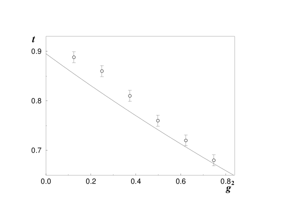
FIG. 1.: Phase diagram for the quantum XY model, Eq. (1), on a square lattice in the $g^{2}\!\!-\!t$ plane at fixed value of $\eta=100$. The line is our result for the undamped system, i.e. $\Gamma_{0}=\Gamma_{1}=0$. The circles are the QMC results of Ref. [3].

Turning to our results, let us consider firstly the behavior of the undamped system ($\widetilde{\kappa}_{n,{\boldsymbol{k}}}=0$). Our phase diagram ($t_{{}_{\rm{BKT}}}$ vs. the square coupling $g^{2}$) for the square lattice is compared with quantum Monte Carlo simulations [3] in Fig. 1. We observe that our approach starts, by construction, from the correct classical value $t^{\rm(cl)}_{{}_{\rm{BKT}}}$ and remains valid as long as ${\cal D}\ll 1$: this means that the reduction of the transition temperature due to the quantum effects can be considered reliable if less than about $30\%$ of $t^{\rm(cl)}_{{}_{\rm{BKT}}}$. On the other hand, the limiting value of the QMC data for vanishing quantum coupling is $0.943$ [3], displaying a significant disagreement with the by now established value $0.895$ quoted above for the classical XY model.

In Fig. 2 the transition temperature versus $g$ is compared with the experimental data both for square and triangular lattices. It must be noticed that the a priori knowledge of the model parameters ($J$, $C_{0}$, and $\eta$) describing the experimental setup is rather poor [7]: therefore there is an uncertainty both on the vertical ($t=T/J$) and on the horizontal [$g$ as given by Eqs. (8 and 7)] scale. Indeed, the values of $J$ used in Ref. [7] give extrapolated classical transition temperatures which are larger than the known theoretical ones, both for the square ($0.95$ against $0.895$) and the triangular ($1.7$ against $1.36$) lattice. In order to avoid such systematic error, each set of data in Fig. 2 is normalized to the corresponding classical extrapolated value, as already done in Ref. [7]. The overall agreement appears to be rather good even though the experiments present a more rapid decrease of the transition temperature for increasing values of $g$: this could suggest that the pure XY model is insufficient to explain this behavior.

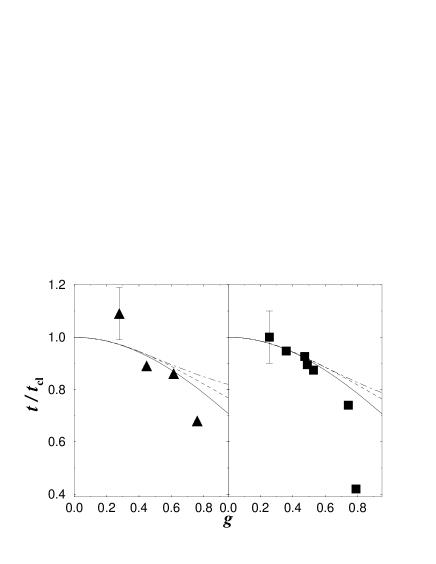
FIG. 2.: Phase diagram for the quantum XY model, Eq. (1), on triangular (on the left) and square (on the right) lattice in the $g\!-\!t$ plane at fixed value of $\eta=100$. Solid line: $\Gamma_{0}=\Gamma_{1}=0$; dashed line: $\Gamma_{0}=3$ and $\Gamma_{1}=0$; dot-dashed line: $\Gamma_{0}=0$ and $\Gamma_{1}=3$. The black squares and triangles are the experimental data of Ref. [7].

Let us now introduce the dissipation. Usually, the damping is described in terms of shunt resistors connecting the islands to ground or/and shunt resistors in parallel to the junctions [18]. Furthermore the environmental coupling is taken to be of Ohmic type, i.e.

$${\hat{\gamma}}_{\boldsymbol{ij}}(s)=\gamma_{\boldsymbol{ij}}=\frac{1}{2\pi}R_{\rm Q}G_{\boldsymbol{ij}}~{}$$ (18)

does not depend on $s$. $R_{\rm Q}=2\pi\hbar/q^{2}$ is the quantum resistance and $G_{\boldsymbol{ij}}$ is the conductance matrix, which reads

$$G_{\boldsymbol{ij}}=\frac{1}{R_{0}}\delta_{\boldsymbol{ij}}+\frac{1}{R_{1}}\,\Big{(}z\,\delta_{\boldsymbol{ij}}-\sum_{\boldsymbol{d}}\delta_{\boldsymbol{i},\boldsymbol{j+d}}\Big{)}~{},$$ (19)

where $R_{0}$ and $R_{1}$ are resistive shunts to the ground and between islands, respectively.

However, a strictly Ohmic damping leads to unphysical results as the logarithmic ultra-violet divergence of the fluctuations of momenta [10, 12], i.e. the number of Cooper pairs in each island. The simplest way to consider the inertia in the response of the dissipation bath is to use the Drude model [10], that consists of a real-time memory damping with exponential decay of the form

$$\gamma(t)=\theta(t)~{}\frac{\gamma}{\tau}~{}e^{-t/\tau}~{},$$ (20)

where $\theta(t)$ is the step function and $\tau^{-1}$ is the Drude ultraviolet cutoff frequency; the Ohmic behavior is recovered in the limit $\tau\ll t$. With this regularization Eq. (18) becomes

$${\hat{\gamma}}_{\boldsymbol{ij}}(s) = \frac{R_{\rm Q}}{2\pi}\bigg{[}\frac{\delta_{\boldsymbol{ij}}}{R_{0}}\,\frac{1}{1+s\,\tau_{0}}$$ (21)

$$+ \frac{1}{R_{1}}\,\Big{(}z\,\delta_{\boldsymbol{ij}}-\sum_{\boldsymbol{d}}\delta_{\boldsymbol{i},\boldsymbol{j+d}}\Big{)}\frac{1}{1+s\,\tau_{1}}\bigg{]}~{}.$$ (22)

The presence of two distinct characteristic times is consistent with the choice of two independent damping mechanism, the on-site and the nearest-neighbor one, related to $R_{0}$ and to $R_{1}$, respectively. The two characteristic times, $\tau_{\ell}$ ($\ell=0,1$), have to be compared with the characteristic times of the equivalent circuit, obtained generalizing the resistively and capacitively shunted junction model [19] to a 2D array, i.e. $R_{0}C_{0}$ and $R_{1}C_{1}$. If $\tau_{\ell}$ is smaller than $R_{\ell}C_{\ell}$ the response of the baths can be considered Ohmic; in the opposite case the behavior of the system is no longer resistive and the inertia in the response of the dissipation bath must be considered. In our calculation, we have therefore assumed $\tau_{\ell}=R_{\ell}C_{\ell}$ as a representative values of the unknown characteristic times of the baths.

In Fig. 2 we have also plotted the modification of the phase diagram due to damping for realistic values of dissipation: we use as dissipation parameters the dimensionless quantities, $\Gamma_{\ell}=R_{Q}/R_{\ell}$. The comparison with the experimental data shows that this kind of dissipation is not very relevant for low values of $g$. Increasing $g$, but remaining in the range where our approach is valid, the dissipation appears to affect the phase diagram in the opposite way with respect to the tendency of the actual experiments. Although our results improve the quantitative accuracy, these agree with the qualitative behavior already found in previous works [18].

The problem of a theoretical explanation of the phase diagram of JJA is thus open, and it might be worthy to investigate whether the common schematization of a Caldeira-Leggett coupling trough the phase variables, Eq. (3), is fully justified from a fundamental point of view for describing a resistive shunt. Moreover, it is also known that dissipation does not have a quenching effect onto the fluctuations of all dynamical variables, as the simple case of the damped harmonic oscillator shows [10], and it might be possible to reasonably modify the mechanism of the environmental interaction in order to reproduce the observed phase diagram.

We thank J.E. Mooij and H.S.J. van der Zant for fruitful correspondence, as well as G. Falci for useful discussions. This work was partly supported by the project COFIN98 of MURST.

REFERENCES

- [1] Proceedings of the ICTP Workshop on Josephson Junction Arrays, edited by H. A. Cerdeira and S. R. Shenoy, Physica B 222(4), 253-406 (1996) and references therein.
- [2] A. I. Belousov and Yu. E. Lozovik, Solid State Commun 100, 421 (1996).
- [3] C. Rojas and J. V. José, Phys. Rev. B 54, 12361 (1996).
- [4] U. Eckern, G. Schön, and V. Ambegaokar, Phys. Rev. B 30, 6419 (1984).
- [5] J. E. Mooij et al., Phys. Rev. Lett. 65, 645 (1990).
- [6] G. Schön and A.D. Zaikin, Phys. Rep. 198, 237 (1990); P. W. Anderson, in Lectures in Many Body Problem, ed. E. R. Caianello (Academic Press, New York, 1964).
- [7] H. S. J. van der Zant, W. J. Elion, L. J. Geerligs and J. E. Mooij, Phys. Rev. B 54, 10081 (1996).
- [8] A. Cuccoli et al., J. Phys.: Condens. Matter 7, 7891 (1995); A. Cuccoli, V. Tognetti, P. Verrucchi, and R. Vaia, Phys. Rev. A 45, 8418 (1992).
- [9] A. O. Caldeira and A. J. Leggett, Ann. Phys. 149, 374 (1983).
- [10] U. Weiss,Quantum Dissipative Systems (World Scientific, Singapore, 2nd edition, 1999).
- [11] J. M. Kosterlitz and D. J. Thouless, J. Phys. C 6, 1181 (1973); J. M. Kosterlitz, J. Phys. C 7, 1046 (1974); V. L. Berezinskii, Zh. Eksp. Teor. Fiz. 59, 907 (1970) [Sov. Phys. JEPT 32, 493 (1971)].
- [12] A. Cuccoli, A. Fubini, V. Tognetti, and R. Vaia, Phys. Rev. E 60, 231 (1999); A. Cuccoli, A. Rossi, V. Tognetti, and R. Vaia, Phys. Rev. E 55, 4849 (1997).
- [13] B. J. Kim and M. Y. Choi, 52, 3624 (1995).
- [14] S. Kim and M. Y. Choi, Phys. Rev. B 41, 111 (1990); 42, 80 (1990).
- [15] A. Cuccoli, V. Tognetti, P. Verrucchi, and R. Vaia, Phys. Rev. B 51, 12840 (1995).
- [16] R. Gupta and C. F. Baillie, Phys. Rev. B 45, 2883 (1992).
- [17] P. Butera and M. Comi, Phys. Rev. B 50, 3052 (1994).
- [18] K-H. Wagenblast et al. in Ref. [1], p. 336; P. A. Bobbert, R. Fazio and G. Schön, Phys. Rev. B 45, 2294 (1992); G. Falci, R. Fazio, and G. Giaquinta, Europhys. Lett. 14, 145 (1991); S. Chakravarty, G-L. Ingold, S. Kivelson and G. Zimanyi, Phys. Rev. B 37, 3283 (1988); M. P. A. Fisher, Phys. Rev. B 36, 3283 (1987); E. Šimánek and R. Brown, Phys. Rev. B 34, 3495 (1986).
- [19] M. Tinkham, Introduction to Superconductivity (McGraw-Hill, New York, 1996); A. Barone and G. Paternò, Physics and applications of the Josephson Effect (Wiley, New York, 1982).