Correlated random band matrices: localization-delocalization transitions

Abstract

We study the statistics of eigenvectors in correlated random band matrix models. These models are characterized by two parameters, the band width $B(N)$ of a Hermitian $N\times N$ matrix and the correlation parameter $C(N)$ describing correlations of matrix elements along diagonal lines. The correlated band matrices show a much richer phenomenology than models without correlation as soon as the correlation parameter scales sufficiently fast with matrix size. In particular, for $B(N)\sim\sqrt{N}$ and $C(N)\sim\sqrt{N}$, the model shows a localization-delocalization transition of the quantum Hall type.

]

I Introduction

In the theory of random Hermitian matrices [1] two robust types of statistics are found in the limit of infinite matrix size (denoted here as ’thermodynamic limit’). First, the Wigner-Dyson statistics describing systems that become ergodic in the thermodynamic limit and have an incompressible, correlated spectrum and Gaussian distributed, uncorrelated amplitudes of the corresponding eigenstates (see Fig. 1a). Since we do not consider further symmetry constraints we focus on the matrix ensembles denoted as class A in the classification of [2]. A convenient representative of its ergodic limiting ensemble is given by the Gaussian unitary matrix ensemble GUE. The second robust statistics is the Poisson statistics with eigenstates, localized on certain basis states (sites), and with an compressible, uncorrelated spectrum (see Fig. 1b).

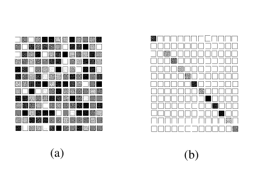
FIG. 1.: Visualization of typical random matrices obeying Wigner-Dyson statistics (a), Poisson statistics (b). The intensity represents the absolute value of matrix elements.

Real complex quantum systems, represented by random Hermitian matrices, can show a crossover between Wigner-Dyson and Poisson statistics or, in some cases, a true quantum phase transition with novel ’critical’ statistics. A well known example is the 3D Anderson model (see Fig. 2)

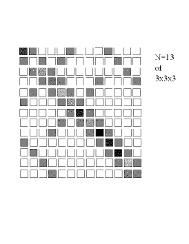
FIG. 2.: Visualization of a typical random matrix obeying the statistics of a 3D Anderson model. The intensity represents the absolute value of matrix elements.

describing the motion of independent electrons on a 3D lattice with random uncorrelated on-site disorder. Below a certain critical value of disorder, in the thermodynamic limit, all states at the energy band center are infinitely extended (delocalized) in space, while for larger disorder all states are spatially localized. Instead of changing the disorder, one can change the energy within the energy band, keeping the disorder fixed at low values. Again, a transition from localization (band tails) to delocalization (band center) occurs. It is worth mentioning, that the average density of states (DOS) is non-critical, i.e. it stays smooth across the localization-delocalization (LD) transition. Although these statements are substantiated by analytical as well as numerical work (for reviews see [3, 4]), the special structure of this matrix ensemble (composed of a sparse, but deterministic matrix and a random diagonal matrix) has prohibited, so far, a rigorous proof of these statements. Another well known system with a transition from localized to critical states is the two-dimensional (2D) quantum Hall system (for reviews see [5, 6]) which we will describe briefly later. Furthermore, several matrix ensembles modeling the motion of 2D disordered electrons undergoing (time-reversal symmetric) spin-orbit interactions are known to display a LD transition (see e.g. [7]). In all of these realistic matrix ensembles the statistics at criticality represents an unstable fixed point under increasing system size (i.e. matrix dimension), which means that any slight shift away from the critical value of the energy, say, will drive the system into one of the stable matrix ensembles, Wigner-Dyson for the delocalized states and Poisson for localized states. The critical ensembles are characterized by correlated spectra, but with a finite compressibility. Furthermore, critical eigenstates are multifractal and the multifractal exponents are related to the compressibility of the spectrum (for a review see [4]).

It is desirable to study matrix ensembles with simple construction rules and to ask for necessary ingredients in order to have a LD transition. Also in quantum chaos the interest in crossover ensembles has grown [8]. In that context the Rosenzweig-Porter model [9] was studied as a toy-model for the crossover. It is defined as a simple superposition of a Poissonian and a Wigner-Dyson matrix. It has been shown rigorously that, by choosing the superposition in an appropriate way, novel critical ensembles emerge, but the spectral compressibility is identical to the Poisson ensemble and states are not multifractal (see [10] and references therein). Another well studied matrix ensemble is that of random band matrices (RBM) with uncorrelated elements. The band width $B$ describes the number of diagonals with non-vanishing elements. For $B\sim N^{s}$, with $s>1/2$, one recovers the Wigner-Dyson statistics. Such band matrix models have been discussed in the context of the ’quantum kicked rotor’ problem [11] and have been studied extensively in a series of papers by Mirlin, Fyodorov and others (for review see [12, 13]). It turned out that, in particular for $B\gg 1$, all states are localized with a localization length (in index space) $\xi\sim B^{2}$. For fixed $B$ one has therefore a crossover from Wigner-Dyson to Poisson statistics as $N$ is taken from values much smaller than $B^{2}$ to values much larger than $B^{2}$, and $B^{2}/N$ is the relevant parameter for a scaling analysis of data. Superpositions of such random band matrices with random diagonal matrices have been studied in the context of the ’two-interacting particle’ problem (see e.g. [14, 15]), however these ensembles do not show novel critical behavior as compared to the Rosenzweig-Porter model.

In fact, only few simply designed matrix ensembles are known to become critical with multifractal critical states (see [16, 17]), for example ’power law’ band matrix ensembles, where the strength of (uncorrelated) matrix elements falls off in a power law fashion in the direction perpendicular to the central diagonal. The critical cases occur for the power law behavior $\sim x^{-1}$ of the typical absolute values of matrix elements [16, 18]. It is, however, important to notice a significant difference to realistic critical ensembles: there is no LD transition within the spectrum; iff parameters are fixed to critical values all states are critical.

In this paper we study correlated random band matrix (CRBM) ensembles and, with the assistance of numerical calculations, argue that these ensembles can lead to a LD transition within the spectrum. A new parameter $C(N)\sim N^{t}$ describing the correlation of certain matrix elements is introduced for random band matrices. For $B(N)\sim\sqrt{N}$ states are localized outside of the energy band center and a LD transition at the energy band center occurs provided $1/2\leq t\leq 1$.

A major motivation for studying these ensemble originates from the theory of the integer quantum Hall effect [6]. The plateau to plateau transition in the quantum Hall effect can be captured in models of non-interacting 2D electrons in a strong magnetic field and a random potential, referred to as quantum Hall system (QHS). In the one-band Landau representation the Hamiltonian is represented as a random matrix with two characteristic features. (i) The matrix elements decay perpendicular to the main diagonal in a Gaussian way. (ii) No correlations exist between elements on distinct ’nebendiagonal’ lines, but Gaussian correlations exist along each of the nebendiagonals. These features led to the introduction of the ’random Landau model’ (RLM) to study critical properties of QHSs (see e.g. [5]). The original purpose of constructing the RLM was to avoid explicite calculations of matrix elements starting from a randomly chosen disorder potential and to directly generate the matrix elements as random numbers that fulfill the statistical properties (i) and (ii). As will be explained in more details below, the corresponding CRBM model simplifies the RLM further, in as much as a sharp band width is introduced and correlations along nebendiagonals are idealized and cutoff after a finite length.

Recently, matrix ensembles with correlated matrix elements attracted some interest [19] in the context of the metal-insulator experiments in 2D [20], for which strong Coulomb interaction is believed to be a necessary ingredient. It is very interesting that in [21] 1D models with correlated disorder potentials could, to a large extent, be solved analytically and that certain correlated disorder potentials were shown to cause LD transitions in 1D. It is not obvious how to extend the method of [21] to the case of CRBM models. Usually, correlations in matrix ensembles lead to serious complications in analytical attacks. For example, in the field theoretic treatment (see e.g. [22]) of random matrix ensembles the absence of long ranged correlations is essential to find appropriate field degrees of freedom that depend smoothly on a single site variable. In our CRBM models correlations are introduced by constraints (a number of matrix elements are taken to be identical). This may help to reduce complications in constructing a field theoretic approach for CRBM models.

In Sec. 2 we give a detailed definition of the CRBM and discuss three alternative interpretations. The investigation of the LD transition is carried out in Sec. 3 by a multifractal analysis of states for an ensemble that is expected to fall into the quantum Hall universality class. Our results are in favor of this expectation. The analysis is carried over to ensembles where correlations are taken to extreme limits in Sec. 4. In Section 5 we present our conclusions.

II Correlated Random Band Matrix Model

Let the elements of a $N\times N$ Hermitian matrix $H$ be written as

$$H_{kl} = x_{kl}+iy_{kl}\;\;{\rm for}\;\;l>k\;,$$ (1)

$$H_{kk} = \sqrt{2}x_{kk}\,,$$ (2)

where all non-vanishing real numbers $x_{kl},y_{kl}$ are taken from the same distribution ${\cal P}$ with vanishing mean and finite variance $\sigma^{2}$. We take the symmetric and uniform distribution on $[-1,1]$ ($\sigma^{2}=1/3$). With $B,C$ being two integer numbers, called the ’band width’ and the ’correlation parameter’, respectively, the correlated band matrix ensembles are defined by the following algorithm (I) – (III) and are visualized in Fig. 3.

(I) Begin with the main diagonal of $H$ and draw a random integer number $N_{1}\leq C$, and the random number $x_{11}$ from the distribution ${\cal P}$. Take the first $N_{1}$ values on the main diagonal equal to $\sqrt{2}x_{11}$. Then, draw $x_{N_{1}+1,N_{1}+1}$ from the distribution ${\cal P}$ and take successively $C$ elements on the main diagonal equal to $\sqrt{2}(x_{N_{1}+1,N_{1}+1})$. Now, draw $x_{N_{1}+C+1,N_{1}+C+1}$ from the distribution ${\cal P}$ and take successively $C$ elements on the main diagonal equal to $\sqrt{2}x_{N_{1}+C+1,N_{1}+C+1}$. Continue with this procedure until the main diagonal is filled up.

(II) Now consider the next ’nebendiagonal’. Its first random element $H_{12}=x_{12}+iy_{12}$ and a random integer number $N_{2}\leq C$ are drawn. Put the first $N_{2}$ elements of this nebendiagonal equal to $H_{12}$. The next $C$ elements on the same nebendiagonal are taken equal to the random value $H_{N_{2}+1,N_{2}+2}$, and so on.

(III) The procedure terminates after the $B$th nebendiagonal ($l-k=B$) is filled up. All other matrix elements ($l-k>B$) are set to zero. Finally, Hermiticity is installed by taking $H_{l>k}=H^{*}_{k<l}$.

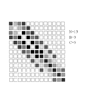
FIG. 3.: Visualization of a typical matrix of the correlated random band matrix model. The intensity represents the absolute value of matrix elements.

For $C=1$ the usual band matrix models (band width $B$) of uncorrelated matrix elements are recovered. $C$ and $B$ form the relevant parameters of the CRBM, while the value of $\sigma$ is not significant – it just defines the energy units. For finite $C>1$ the correlation along (neben)diagonals is a triangular function of range $C$ and half-width $C/2$. Thus, $C/2$ is a typical distance over which elements are correlated along (neben)diagonals. The spectrum is always distributed in a symmetric way around the center $E=0$ as a consequence of the symmetry of the distribution ${\cal P}$.

In the following, we are going to discuss three possible physical interpretations. The most obvious interpretation relies on the site representation $\left.\mid l\right\rangle=(0,0,\ldots,l=1,0,\ldots,0)$. In this representation, $H$ describes hopping of particles on a 1D chain of length $L=N$ (lattice spacing $=1$) with a maximum distance of hopping equal to $B$. The average hopping probability in one instant of time $t$ is ($\hbar=1$, $\left\langle\ldots\right\rangle$ denotes the ensemble average)

$$\left\langle|\left\langle k(t)|l(t+1)\right\rangle|^{2}\right\rangle=\sigma^{2}\;\;{\rm for}\;\;0\leq|l-k|\leq B\,.$$ (3)

FIG. 4.: One-dimensional interpretation of correlated band matrices. Hopping events for distinct hopping distances are uncorrelated. Hopping events for the same hopping distance are correlated over typically $C/2$ nearest neighbors. In this example $B\geq 6$, $C\geq 3$.

The correlation between matrix elements means that two hopping amplitudes are identical, if the hopping distance is equal, and provided the hopping starts at sites the distance between which is less than typically $C/2$ (see Fig. 4).

An alternative interpretation results, when the $N$ sites are arranged in a quasi-1D (Q1D) geometry with $N_{c}=B+1$ parallel ’channels’ in a ’wire’ of length $L^{\prime}=N/(B+1)$. The lattice spacing along the wire, $\hbar$, and the unit of time are taken to be $1$. Transitions in one unit of time are possible between channels (coupling) and along the wire (hopping). Sites are labeled (see Fig. 5) such that hopping is possible at most over one lattice spacing along the wire. Again, hopping (coupling) is correlated over typically $\sim C/2$ states, provided the difference between labels is identical.

FIG. 5.: Quasi-one-dimensional interpretation of correlated random band matrices. Sites are labeled such that for a fixed cross section of the wire all channels are filled up with sites, before one proceeds to the next cross section. Hopping events along the wire and couplings within each cross section are uncorrelated, if label distances are distinct. For identical label distances they are correlated over typically $C/2$ sites. In this example $B=3$, $C\geq 2$.

A less obvious interpretation of CRBM models arises when quantum Hall systems are studied in a one band Landau representation. A quantum Hall system is described by a one-particle Hamiltonian of 2D electrons (charge $-e$, mass $m$) in the presence of a strong perpendicular magnetic field ${\cal B}$ and a random potential $V(x,y)$. In Landau gauge the Hamiltonian reads

$$H=\frac{1}{2m}\left(p_{x}^{2}+(p_{y}+e{\cal B}x)^{2}\right)+V(x,y)\,,$$ (4)

where $(p_{x},p_{y})$ is the canonical momentum with respect to the Cartesian coordinates $(x,y)$. For periodic boundary conditions in $y$-direction (length $L_{y}$) the kinetic energy forms a highly degenerate harmonic oscillator problem ($p_{y}$ is conserved) that is diagonalized by Landau states [23] $\left.\mid n,l\right\rangle$. Here $n=0,1,2,3,\ldots$ labels the Landau energies $E_{n}=\hbar\omega_{c}(n+1/2)$ ($\omega_{c}=e{\cal B}/m$ cyclotron energy), and $l=0,1,2,\ldots$ labels center coordinates of the degenerate Landau states. The Landau states are separated into plane waves in $y$-direction with quantized momentum $q_{l}$ and into oscillator wave functions centered at $X_{l}=-\lambda^{2}q_{l}$, where $\lambda=\sqrt{h/(e{\cal B})}$ is the characteristic ’magnetic length’. As long as the typical values of the random potential are much smaller than the cyclotron energy, one can study the full eigenvalue problem of the low lying ’Landau bands’ approximately by restricting the Hilbert space to separate Landau levels $n$. In particular, for the lowest Landau level the Landau states read

$$\left\langle x,y|l\right\rangle=\frac{1}{\pi^{1/4}\sqrt{\lambda L_{y}}}\exp\left\{{-i\frac{X_{l}y}{\lambda^{2}}}\right\}\exp\left\{{-\frac{(x-X_{l})^{2}}{2\lambda^{2}}}\right\}\,.$$ (5)

A convenient recipe to study finite systems of length $L$ in $x$-direction is to use ’Landau counting’ of states, that is to take only those Landau states into account for which the center coordinates $X_{l}$ fall into the interval $[0,L]$. The total number of states, for an aspect ratio $a=L_{y}/L$, is

$$N=(a/2\pi)(L/\lambda)^{2}\,.$$ (6)

By shifting the lowest Landau energy to zero, the eigenvalue problem is defined by the matrix $H_{kl}=\left\langle k|V|l\right\rangle$ which reads

$$H_{kl}=\frac{e^{-\frac{1}{4\lambda^{2}}(\Delta X)^{2}}}{\sqrt{\pi}\lambda}\int\limits_{-\infty}^{\infty}dx\,\tilde{V}(x;\Delta X)e^{-\frac{1}{\lambda^{2}}(x-X)^{2}}\,,$$ (7)

$$\tilde{V}(x;\Delta X)\equiv L^{-1}_{y}\int\limits_{-{L_{y}/2}}^{L_{y}/2}dy\,V(x,y)e^{iy\Delta X/\lambda^{2}}\,,$$ (8)

where $X=(X_{k}+X_{l})/2$ and $\Delta X=X_{k}-X_{l}$. These matrix elements form a random $N\times N$ matrix, the elements of which are composed by a Fourier transformation of the random potential in $y$-direction and a Gaussian weighted averaging of the potential over a magnetic length in $x$-direction. Crucial for the structure of the matrix is the fact that, within the distance of one magnetic length $\lambda$, a number of $N_{\lambda}\sim N(\lambda/L)$ different Landau states can be situated (see Fig. 6). Thus, for a constant aspect ratio, this number increases as $N_{\lambda}\sim\sqrt{N}$ in the thermodynamic limit.

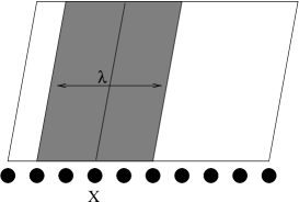
FIG. 6.: Interpretation of correlated band matrices as quantum Hall system. Bare states are interpreted as Landau states on a 2D plane. The qualitative properties of Landau states are shown: plane waves in $y$ direction situated at center coordinate $X_{l}$, extended in $x$-direction over approximately one magnetic length $\lambda$ corresponding to $N_{\lambda}$ neighboring states.

This leads to correlations between matrix elements along nebendiagonals over a range of $N_{\lambda}$ states. This range increases when the disorder potential is correlated in real space over distances exceeding the magnetic length. The correlation between matrix elements on distinct (neben)diagonals is negligible, since the correlator contains the superposition of $\sim N_{\lambda}$ random phase factors. The matrix elements decay perpendicular to the main diagonal due to the Gaussian decay of Landau states. For disorder potentials with a spatial correlation length $d\gg\lambda$ the decay sets in earlier, because the Landau states are orthogonal. A quantitative analysis shows (see [5]) that the Gaussian band-width is

$$\tilde{B}=\frac{1}{\beta}\sqrt{\frac{aN}{\pi}}$$ (9)

and the Gaussian correlation length along (neben)diagonals is

$$\tilde{C}=\beta\sqrt{\frac{aN}{\pi}}\,.$$ (10)

Here $\beta\geq 1$ is a parameter that is controlled by the potential correlation length $d$,

$$\beta\equiv\frac{\sqrt{d^{2}+\lambda^{2}}}{\lambda}\,.$$ (11)

For finite and fixed values $d,a$, in the thermodynamic limit, $\tilde{B}(N)$ and $\tilde{C}(N)$ increase as $\sqrt{N}$ to infinity. A matrix for QHSs with the statistical properties described above is denoted as ’random Landau matrix’ (RLM) (see [5]).

Our CRBM simulates the RLM in as much, as it has the same qualitative features of a finite band width $B$ and a correlation length, being typically $C/2$. The quantitative differences are that, in the CRBM, the matrices have a sharp band width $B$, instead of a Gaussian band width $\tilde{B}$, and that the correlation function is a triangle with a half width $C/2$, instead of a Gaussian with a half width $\tilde{C}$. In the thermodynamic limit, however, we expect that these differences should be insignificant for the statistics of eigenvalues and eigenvectors, provided the parameters $B(N)$ and $C(N)$ scale in the same way with $N$ as the parameters $\tilde{B}(N)$ and $\tilde{C}(N)$, respectively. Note, however, that in the RLM the ratio $\tilde{C}(N)/\tilde{B}(N)=\beta^{2}$ is bounded from below by 1, while in the CRBM model we are free to choose any value for $B(N),C(N)$.

III Multifractality and Spatial Correlations

To study the LD properties of matrix ensembles numerically, one can follow a number of different strategies. The most efficient is to analyze only the eigenvalue statistics. Although the eigenvalues encode most of the relevant information about LD properties, the statistics of wavefunction amplitudes is more direct. Localization, delocalization and even criticality of states can be qualitatively distinguished already by inspection of plots of the squared amplitudes of wavefunctions (see e.g. Fig. 7). Critical states $\psi({\bf r})$ are characterized by having a multifractal distribution of its squared amplitudes ${\rm prob}({\bf r})\equiv|\psi({\bf r})|^{2}$. This spectrum becomes independent of system size and is universal for all of the critical states in the thermodynamic limit (for a review see [24]) or, more generally, follows a universal distribution ( see [25]). In particular, the geometric mean is a convenient measure of a typical probability and scales as

$${\rm prob}_{\rm typ}=\exp\left\langle\ln({\rm prob({\bf r})})\right\rangle\sim L^{-{\alpha_{0}}}\,,$$ (12)

where the deviation $\alpha_{0}-d\geq 0$ of the fractal dimension $\alpha_{0}$ from the Euclidean dimension $d$ signals multifractality and is the most sensitive critical exponent of the LD transition. Although a critical state is extended all over the system, it fluctuates strongly and has large regions of low probability which results in the stronger decay of typical amplitudes as compared to homogeneously extended states. A quantity that is closely related to $\alpha_{0}$ is the exponent $\eta$ of long ranged spatial correlations $\left\langle{\rm prob}(r){\rm prob}(0)\right\rangle\sim r^{-\eta}$ [26, 27]. It fulfills scaling relations to the fractal dimension of the second moment of ${\rm prob}({\bf r})$ [28], and also to the compressibility of the eigenvalue spectrum [29] (see also [30]). As a crude estimate (based on a log-normal approximation[28] to the distribution of ${\rm prob}$) one has $\eta\approx 2(\alpha_{0}-d)$.

In this work we focus on wavefunction statistics and the determination of $\alpha_{0}$. One should, however, be careful when drawing conclusions from the calculation of fractal exponents for finite matrix sizes. Such calculations should be assisted by inspection of states, and one should study the dependence on the matrix size $N$. For example, states with localization lengths that are small, but not very small compared to system size tend to produce larger values of $\alpha_{0}$ because parts of the wave function have low amplitudes. This can be seen easily in plots of the corresponding squared amplitudes. From the linear regression procedure that allows to determine $\alpha_{0}$ one cannot distinguish such behavior from true multifractality, as long as the system sizes cannot be made much larger than the localization length. Furthermore, one should distinguish between spatial, energy, and ensemble averages. In practice, we first perform the spatial average for a fixed wavefunction to determine the exponent $\alpha_{0}$ for a finite matrix size $N$ by the box-counting method (see e.g. [28]). This can be done for many states in the critical region (which has finite width for finite $N$) and we average over these states. Finally, an average over different realizations (ensemble average) can be performed. It is not obvious, that the order of these different procedures commutes since the exponent fluctuates from state to state. The question about the self-averaging of the fractal exponents was recently addressed in [25] and it was claimed that exponents follow a universal scale independent distribution function in the thermodynamic limit, rather than being self-averaging. We do not investigate this question here. For our finite systems the exponents are fluctuating anyway and we consider averages (over typically 100 states) as explained above.

For a number of different models of QHSs the exponent $\alpha_{0}$ has been determined, e.g $\alpha_{0}=2.28\pm 0.02$ in [31]. Other authors (e.g. [32]) find values between $2.27\pm 0.1$ and $\alpha_{0}=2.29\pm 0.02$. The largest system sizes studied were about $L\approx 200\lambda$ leading to matrix dimensions $N$ of about $10^{4}$.

For the sake of a direct comparison of wavefunction plots between our CRBM models and the RLM we took the 2D Landau representation of Eq. (5) with a Landau counting for an aspect ratio $a=1$. The eigenvalues and eigenstates were calculated numerically exploiting the band structure of the matrices. To be as close as possible to a real QHS with an aspect ratio $a\approx 1$ and a short ranged random potential, we took $B(N)=\tilde{B}(N,a=1,\beta=1)=\sqrt{N/\pi}$ and $C(N)=(1/2)\tilde{C}(N,a=1,\beta=1)=(1/2)\sqrt{N/\pi}$ (e.g. the largest matrices had parameters $N=6400$, $B=45$ and $C=90$). We refer to this choice of parameters as the ”standard quantum Hall case”

Our findings for the standard quantum Hall case of the CRBM model can be summarized as follows. Almost all states are localized (see Fig. 7a). Only those around the energy band center $E=0$ are multifractaly extended (see Fig. 7b).

FIG. 7.: Squared amplitudes of a localized state (a), and a critical state (b), in the correlated random band matrix model for the standard quantum Hall case. States are represented in two-dimensional Landau representation.

For finite $N$ there is a small energy band of extended states with localization length $\xi\geq L$. The energy band width of extended states, $\Delta_{c}$, shrinks with increasing $N$ with a critical exponent related to the divergence of the localization length at the band center. To determine this critical exponent it would be sufficient to determine $\Delta_{c}$ as a function of system size. However, $\Delta_{c}$ can be defined only by considering an appropriate scaling variable, e.g the participation ratio, that increases above some threshold value when the states become extended. In finite systems scaling variables are strongly fluctuating and one has to consider distribution functions and/or appropriate typical values. We did not try to calculate this exponent precisely, but only convinced ourself that the typical numbers of clearly extended states was comparable to those of realistic quantum Hall systems with $\tilde{B}(N)=B(N)$, $\tilde{C}(N)=2C(N)$.

The fluctuation of $\alpha_{0}$ determined by the box-counting for individual states can bee seen in Fig. 10. The average over 100 different extended states of a $N=6400$ standard quantum Hall case yields $\alpha_{0}=2.26\pm 0.02$. This value is close to the value $\alpha_{0}=2.28\pm 0.02$ obtained by the same averaging procedure for an original quantum Hall system in [31]. We therefore conclude, that the CRBM shows indeed a LD transition reminiscent of quantum Hall systems. It seems likely that, in the thermodynamic limit, the critical behavior of CRBMs in the standard quantum Hall class is actually identical to that of the quantum Hall universality class, because the essential $N$ dependence of the relevant parameters, band width $B(N)\sim\sqrt{N}$ and correlation parameter $C(N)\sim\sqrt{N}$, are identical to those of realistic QHSs in Landau representation.

So far the comparison of multifractal exponents was based on the wave function statistics without any reference to spatial correlations. Therefore, a more ambitious comparison between the CRBM and a QHS concerns the critical exponents of spatial correlations and their scaling relations to the multifractal exponents. In a multifractal state the $q$-correlator $\left\langle{\rm prob}^{q}(r){\rm prob}^{q}(0)\right\rangle\sim r^{-x(q)}$ has fractal dimension

$$x(q)=2\Delta(q)-\Delta(2q)$$ (13)

where $\Delta(q)$ are the usual fractal exponents of the $q$-moments $\left\langle{\rm prob}^{q}({\bf r})\right\rangle\sim L^{-\Delta(q)}$ (for review see [4]).

We find for the spatial correlations of the standard quantum Hall case the scaling exponents shown in Fig. 8. They are compared with the data that follow from the spectrum $\Delta(q)$ and Eq. (13). The spectrum $\Delta(q)$ was calculated by the box counting-method.

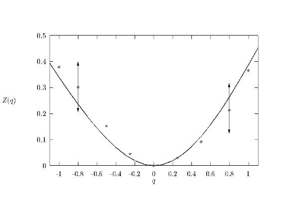
FIG. 8.: Numerically obtained correlation exponents $z(q)$ (symbols) in comparison with the data following from the scaling relation (13) (line). Error bars are shown for two representative values.

They satisfy, within the numerical uncertainties, the scaling relation Eq. (13). Furthermore, the exponents are close to their values for critical states in realistic quantum Hall systems [31], e.g. the exponent of ’anomalous diffusion’ [27] is $x(1)=0.4\pm 0.1$.

We summarize this section by stating that our multifractal analysis gives a number of clear indications that correlated random band matrices, in the ”standard quantum Hall” case, are true representatives of the quantum Hall universality class.

We close this section with an observation not directly relevant for the questions addressed in this paper, but which may be relevant for those readers that like to perform numerical calculations with the CRBM model. In realistic QHSs with an aspect ratio $a\not=1$ one observes that a number of the multifractal states tend to have an orientation along the direction of smaller width. This orientation effect has no influence on the asymptotic statistical properties of the wave function amplitudes as $N$ scales to $\infty$. Only corrections to scaling due to finite system sizes can be different for different aspect ratios. However, an aspect ratio $a\not=1$ will influence scaling variables like the Thouless sensitivity $g_{\rm Th}=\delta\varepsilon/\Delta$. It measures the change in energy $\delta\varepsilon$ due to a change from periodic to antiperiodic boundary conditions in a given direction, relative to the mean level spacing $\Delta$. It is exponentially small for localized states and typically of order 1 for critically extended states. We calculated this quantity for a realistic quantum Hall system. It has strong mesoscopic fluctuations (variance $\sim$ mean) and found that the unique maximum of its typical values at the band center, for $a=1$, splits up into two maxima, for $a\not=1$, symmetric around the band center. This behavior is related to the fact that those wave functions that start to be extended in the direction of smaller width are more sensitive to changes in the boundary condition than those that have already huge localization lengths and are uniformly extended in both directions. In the CRBM model we observe a similar phenomenon. For the standard quantum Hall case we actually found a tendency for an orientation into the $y$-direction (with Landau states as defined in Eq. (5) and Landau counting for $a=1$)). This behavior changes to an orientation in the opposite direction under increasing $C(N)$ by a factor of ${\cal O}(1)$, keeping $B(N)$ fixed. In contrast to a realistic QHS where we can calculate $\tilde{B},\tilde{C}$ for a truly symmetric situation, $a=1$, in the CRBM model we do not know a priori if the choice $C/2=B$ is appropriate to simulate a truly symmetric situation, $a=1$. Because the identification of the half-width value of a triangular correlation function with the half-width of a Gaussian is not strict, taking a factor of order unity between them is equally well justified. The same ambiguity is present in the identification of the band width $B$ with $\tilde{B}$. Any change in $B$, $C$ by a factor of order unity can therefore lead to the orientation effect. As in realistic quantum Hall systems we also found the splitting of the maximum in Thouless sensitivities in the standard quantum Hall case. This splitting effect may be further investigated.

IV Tuning the Correlation Parameter $C(N)$

When the correlation parameter is fixed to a constant $C(N)\equiv C_{0}$ the CRBM will behave like an ordinary random band matrix when $N\gg C_{0}$. This case is very well understood (see [12, 13]) and one knows that a crossover from localization to Wigner-Dyson delocalization takes place as the band width $B$ is varied. The localization length in 1D interpretation is $\xi_{\rm 1D}=cB^{2}$ ($c$ a constant of order unity). Except for the far energy band tails, where states are stronger localized, the localization behavior is almost uniform over the energy band. It is worth noting that the amplitudes of wavefunctions within the central region (where the amplitudes are not exponentially small) are strongly fluctuating, but they are not multifractal in the limit of large $B(N)$. The entire distribution of amplitudes is, asymptotically in $B$, fixed by the value of the ratio $g=\xi_{\rm 1D}/N=cB^{2}(N)/N$. This ratio is the relevant scaling parameter and is denoted as ”conductance”. As we have seen in the previous section, the behavior of CRBM changes drastically when the correlation parameter increases sufficiently fast with $N$. In the standard quantum Hall case, a LD transition takes place within the energy band. To get more insight into the role of the correlation parameter we therefore studied two extreme cases: (A) $C(N)=1$, and (B) $C(N)=N$. In both cases we kept $B(N)\sim\sqrt{N}$ as in the standard quantum Hall case.

Situation (A) corresponds to the usual uncorrelated random band matrix models with a large localization length of $\xi_{\rm 1D}\sim B^{2}\sim L$ in 1D-interpretation ($\xi_{\rm Q1D}\sim B\sim L^{\prime}$ in Q1D-interpretation) and a constant ’conductance’ of order $1$, $g=\xi_{\rm 1D}/L=\xi_{\rm Q1D}/L^{\prime}={\rm const}$. This model has no interpretation as a QHS, since the ratio $C(N)/B(N)\sim N^{-1/2}\ll 1$. For better comparison we used the same Landau representation as before and performed a multifractal analysis of the extended states by the same box-counting method as in the standard quantum Hall case.

Our findings in situation (A) can be summarized as follows. All states behave similar within the band (except for those in the far tails) The states are not uniformly extended, but are confined to strips with a width of about half the system size (see Fig. 9). Within that strip the states are extended and they fluctuate strongly in a ’grassy’ way. They do not show the self-similar regions of low amplitude like typical multifractal states.

FIG. 9.: Squared amplitudes of a typical state in the random band matrix model for situation (A) with vanishing correlation between matrix elements. The state is represented in the two-dimensional Landau representation.

This behavior is compatible with the 1D (or quasi-1D) interpretation of the uncorrelated random band matrix with a localization length of the order of $L$ ($L^{\prime}$) and a conductance of order unity. We calculated, for $N=6400,B=45$, the exponent $\alpha_{0}^{[2D/C=1]}\approx 2.14$ (see Fig. 10). This value must be taken with care, as the states were not extended over the full system. They are localized to an area of about half the system size. Thus, the regions of exponentially small amplitudes outside the localization center lead to values $\alpha_{0}>2$. Taking amplitudes from only the localization center reduces the average of $\alpha_{0}$, but fluctuations from state to state are strong. We therefore expect that $\alpha_{0}$, measured in the localization center, will slowly converge to $\alpha_{0}=2$ as $B(N)$ increases further with $N$.

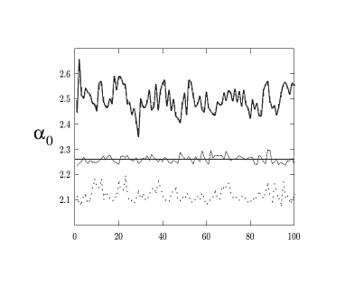
FIG. 10.: Multifractal exponents for 100 extended states of correlated random band matrix models in the standard quantum Hall case (middle), in situation (A) (bottom) and in situation (B) (top). The straight line corresponds to the average in the standard quantum Hall case.

Situation (B) deviates strongly from the usual uncorrelated random band matrix models. The elements on each (neben)diagonal are constant, but uncorrelated for distinct (neben)diagonals. We denote them by $h_{m}$ where m=0 labels the main diagonal and positive (negative) $m$ label the upper right (lower left) lying nebendiagonals.

Had we set $N=\infty$ in the first place, we could solve the eigenvalue problem by Fourier transformation. Each hopping event over a fixed distance would be translational invariant. Thus, the eigenstates, for $N=\infty$, are plane waves $\psi_{q}(l)=e^{iql}$ where $q$ is a quantum wave number that can take any real value. The corresponding eigenvalue is

$$E_{q}=\sum_{m=-\infty}^{\infty}h_{m}e^{iqm}=h_{0}+2\Re\sum_{m=1}^{B}h_{m}e^{iqm}\,.$$ (14)

In Landau representation the plane waves $\psi_{q}(l)$ transform into wave functions $\psi_{q}(x,y)$ that are plane waves in $x$ direction, centered at a center coordinate $Y_{q}=-\lambda q$, and have a width of a magnetic length in $y$ direction.

For any finite $N$, however, such solution is not possible, unless periodic boundary conditions are implemented in the site representation. To implement them into our band matrix models we have to add $\sim B^{2}$ matrix elements in the upper right (and lower left) corners of the matrix. This would violate the band structure. We see that, for any finite $N$, the correlated band-matrix brakes the translational invariance of hopping events, and it is not obvious that the states restore this symmetry when $N$ goes to infinity. Actually, our finite $N$ results indicate that the states will not be plane waves in the center of the band (see Fig. 11). Furthermore, a simple perturbative treatment shows that the omission of the $\sim B^{2}$ elements in the corners cannot be neglected in the limit $N\to\infty$.

The CRBM in situation (B) does also allow for an interpretation as a quantum Hall system, since $C(N)/B(N)\sim\sqrt{N}>1$. As follows from equations (9 – 11) the potential correlation length $d\sim N^{1/4}$ and the aspect ratio is large, $a\sim\sqrt{N}$. This translates to the scaling with system size $L$ as

$$d\sim L\sim N^{1/4},\;L_{y}=aL\sim L^{3}\,.$$ (15)

The CRBM in situation (B), thus represents a long quantum Hall strip where $L_{y}/L\sim(L/\lambda)^{2}$ and the random potential can be thought of as being smooth over a distance of the width $L$. With periodic boundary conditions in $x$-direction one would again conclude that eigenstates are plane waves in $x$-direction, labeled by $N$ different center coordinates $Y_{q}$ ($q$ is an integer times $2\pi/L$) in $y$-direction, and the eigenvalues $E_{q}$ would be determined by the value of the random potential at center coordinate $Y_{q}$. This scenario is also consistent with Eq. (14), because the Fourier transform of the random potential at $V(Y_{q})$ yields the matrix elements $h_{m}$ (see also Eq. 8). In the absence of periodic boundary conditions the situation changes. For energies far from the band center one expects, that the corresponding eigenstates are localized on equipotential contours of the random potential and are centered at some value $Y_{q}$. However, close to the energy band center eigenstates become extended and one typical eigenstate is shown in Fig. 11.

FIG. 11.: Squared amplitudes of a typical state in the random band matrix model for situation (B) with strongest correlation between matrix elements. The state is represented in the two-dimensional Landau representation.

Although this state has a preferred orientation in $x$-direction it is by no means localized to a small region in $y$-direction. It fluctuates strongly, it has non-vanishing values all over the system, and it also shows large areas of low probability. Therefore, the multifractal exponent $\alpha_{0}$ is larger than in the standard quantum Hall situation.

Let us try to give heuristic arguments of how to estimate the value of $\alpha_{0}$. For that purpose we recall that, quite generally $\xi_{\rm Q1D}$ is of the order of the number of transverse modes $N_{c}$ times the relevant scattering length $l$ (for a discussion see e.g. [4]). In our situation $N_{c}=N$ and $l\approx d\sim L$. Therefore, the quasi-1D localization length is estimated to be $\sim L_{y}^{5/3}$, and it is much larger than $L_{y}$ [33]. We may thus assume that the state is critical and has, in the strip-representation, a value $\alpha_{0}\approx 2.26$ when the fractal analysis is restricted to sizes much larger than $d\sim L$. Recall that we have chosen the Landau representation corresponding to an aspect ratio $a=1$. Therefore, the value of $\alpha_{0}$ found by box counting in that representation must be different. The box counting method uses squares of size $l^{2}$ in the 2D Landau representation with $a=1$. This corresponds to rectangular boxes in the strip-representation, where the length in $y$ direction scales as the third power of the length in $x$-direction. Thus, the ”effective volume” is $l^{4}$. By this reasoning $\alpha_{0}(C=N)-2$ will be, in the $a=1$ representation, two times larger than in the strip-representation, and we may expect that we should find $\alpha_{0}^{[C=N]}\approx 2.54$ by box-counting in 2D Landau representation with $a=1$. Indeed, this estimate is compatible with our findings as displayed in Fig. 10.

V Conclusions

We have studied a novel type of matrix models, the correlated random band matrices. We used numerical diagonalization and performed a multifractal analysis to analyze the localization-delocalization properties of such matrix models in the thermodynamic limit of infinite matrix size.

The parameters of correlated band matrices are the band width $B$ and the correlation parameter $C$. We offered three interpretations: (i) independent quantum particles on a one dimensional chain with correlated hopping, (ii) independent quantum particles on a quasi-one-dimensional strip with correlated coupling of channels, and (iii) in some range of its parameters the models resemble two dimensional quantum Hall systems. For $B\sim C\sim\sqrt{N}$ a transition from localized to critical states in the band center occurs, and the corresponding critical exponents are close to those of real quantum Hall systems. Furthermore, we found the following qualitative behavior when keeping the band width $\sim\sqrt{N}$ constant: A reduction of correlations suppresses multifractality (i.e. criticality) at the band center and finally, for $C=1$, the ordinary non-critical random band matrix ensemble is reached which shows localization lengths $\xi\sim B^{2}$. Increasing correlations beyond $C\sim\sqrt{N}$, the transition to critical states in the band center remains, however their multifractality seems to be more pronounced. The fractal critical exponent for extreme correlations, $C(N)=N$, turned out to be compatible with a heuristic estimate.

Therefore, our numerical results suggest that the correlated band matrix models show transitions from localization to critical delocalization on approaching the energy band center, provided the band width scales like $B(N)\sim\sqrt{N}$ and the correlation parameter scales like $C(N)\sim N^{t}$ with $1/2\leq t\leq 1$. It should be pointed out that correlations lead to stronger localization off the band center, while they lead to critical delocalization at the band center.

We hope that our work initiates more studies on the ensemble of correlated random band matrices with a general behavior of $B(N)\sim N^{s}$, $C(N)\sim N^{t}$ where $s,t$ may vary between $0$ and $1$, and to reach solid statements about the localization behavior in the thermodynamic limit. We also like to point out, that the ”standard quantum Hall case” of the correlated random band matrix models is not only a simple matrix realization for quantum Hall systems, but has a very interesting distinction from other representative models for the quantum Hall universality class (for an overview over such models see [34]). The correlated random band matrix does not incorporate any handedness related to the magnetic field. This handedness is essential in all other representative models that allow for the existence of extended states. In the correlated random band matrix model, however, the connection to a quantum Hall system goes via the Landau representation, which takes the handedness into account. Fortunately, the question of localization and delocalization is not restricted to that representation. In the correlated band matrix model the correlation of matrix elements is the key for the quantum Hall transition. It would be very interesting to construct a manageable field theoretic formulation for the correlated random band matrix model. This may be possible when taking advantage of the fact that the correlations are given by constraints which may be included by Lagrangian multipliers.

Acknowledgment. MJ thanks B. Shapiro for previous collaboration on matrix models related to the quantum Hall effect and for the central idea to construct the ensembles of correlated random band matrices. We thank J. Hajdu, B. Huckestein, F. Izrailev and I. Varga for useful discussions. This research was supported in part by the Sonderforschungsbereich 341 of the DFG and by the MINERVA foundation.

REFERENCES

- [1] T. Guhr, A. Mueller-Groeling, and H.A. Weidenmüller, Phys. Rep. 299, 189 (1998)
- [2] M.R. Zirnbauer, J. Math. Phys. 37, 4986 (1996); A. Altland, and M.R. Zirnbauer, Phys. Rev. B 55, 1142 (1997)
- [3] B. Kramer, and A. MacKinnon, Rep. Prog. Phys. 56, 1469 (1993)
- [4] M. Janssen, Phys. Reports 295, 1 (1998)
- [5] B. Huckestein, Rev. Mod. Phys. 67, 357 (1995)
- [6] M. Janssen, O. Viehweger, U. Fastenrath, and J. Hajdu, Introduction to the Theory of the Integer Quantum Hall Effect, VCH-Verlag, Weinheim, 1994
- [7] R. Merkt, M. Janssen, and B. Huckestein, Phys. Rev. B 58, 4394 (1998)
- [8] E.B. Bogomolny, C. Gerland, and C. Schmit, Phys. Rev. E 59, R1315 (1999), and references therein
- [9] N. Rosenzweig, and C.E. Porter, Phys. Rev. 120, 1698 (1960
- [10] M. Janssen, B. Shapiro, and I. Varga, Phys. Rev. Lett. 81, C3048 (1998)
- [11] F.M. Izrailev, Phys. Reports 196, 299 (1990)
- [12] Y.V. Fyodorov, and A.D. Mirlin, Int. J. Mod. Phys. B 8, 3795 (1994)
- [13] A.D Mirlin, cond-mat/9907126
- [14] D.L. Shepelyansky, Phys. Rev. Lett. 73, 2607 (1994)
- [15] K.M. Frahm, Eur. Phys. J B 10, 371 (1999)
- [16] A.D. Mirlin, Y.V. Fyodorov, F.-M. Dittes,J. Quezada, and T.H. Seligman, Phys. Rev. E 54, 3221 (1996)
- [17] V.E. Kravtsov, and K.A. Muttalib, Phys. Rev. Lett. 79, 1913 (1997)
- [18] I. Varga, and D. Braun, cond-mat/9909285
- [19] V.V. Flambaum, and V.V. Sokolov, cond-mat/9904013
- [20] S.V. Kravchenko, W.E. Mason, G.E. Bowker, J.E. Furneaux, V.M. Pudalov, and M. D’lorio Phys. Rev. B 51, 7038 (1995)
- [21] F.M. Izrailev, and A.A. Krokhin, cond-mat/9812209
- [22] K.B. Efetov, Supersymmetry in Disorder and Chaos, Cambridge University Press, New York, 1997
- [23] L. Landau, Z. Physik 64, 629 (1930)
- [24] M. Janssen, Int. J. Mod. Phys. 8, 943 (1994)
- [25] D.A. Parshin, and H.R. Schober, cond-mat/9907067
- [26] F. Wegner, Z. Physik B 36, 209 (1980)
- [27] J.T. Chalker, and G.J. Daniell, Phys. Rev. Lett. 61, 593 (1988)
- [28] W. Pook, and M. Janssen, Z. Physik B 82, 295 (1991)
- [29] J.T. Chalker, V.E. Kravtsov, and I.V. Lerner, JETP Lett. 64, 386 (1996)
- [30] D.G. Polyakov, Phys. Rev. Lett. 81, 4696 (1998)
- [31] K. Pracz, M. Janssen, and P. Freche, J. Phys. Condensed Matter 8, 7147 (1996)
- [32] R. Klesse, and M. Metzler, Europhys. Lett. 32, 229 (1995); B. Huckestein, L. Schweitzer, and B. Kramer, Surface Sciences 263, 125 (1992)
- [33] This is in contrast to a quantum Hall strip of width and much larger length , for which the potential correlation length . In that case one knows from many numerical simulations that the quasi-1D localization length is of the order of for critical states (see e.g. [5]).
- [34] M.R. Zirnbauer, cond-mat/9905054