Persistence exponents
of non-Gaussian processes
in statistical mechanics

Abstract

Motivated by certain problems of statistical physics we consider a stationary stochastic process in which deterministic evolution is interrupted at random times by upward jumps of a fixed size. If the evolution consists of linear decay, the sample functions are of the ”random sawtooth” type and the level dependent persistence exponent $\theta$ can be calculated exactly. We then develop an expansion method valid for small curvature of the deterministic curve. The curvature parameter $g$ plays the role of the coupling constant of an interacting particle system. The leading order curvature correction to $\theta$ is proportional to $\sim g^{2/3}$. The expansion applies in particular to exponential decay in the limit of large level, where the curvature correction considerably improves the linear approximation. The Langevin equation, with Gaussian white noise, is recovered as a singular limiting case.

L.P.T. – ORSAY 99/70
¹Laboratoire associé au Centre National de la Recherche Scientifique - UMR 8627

1 Introduction

In this work we study the stationary stochastic process $\xi(t)$ that obeys the equation

$$\frac{\mbox{d}\xi(t)}{\mbox{d}t}=-A(\xi)+a\,\sum_{\ell}\delta(t-t_{\ell})$$ (1)

Here $a$ is a positive parameter and the $t_{\ell}$ are random times distributed independently and uniformly with density $\rho$; the random term therefore represents white noise, but with a nonzero average equal to $\rho a$. Hence $\xi(t)$ evolves deterministically except for upward jumps of fixed size $a$ occurring at random times. We take the systematic ”force” $A(\xi)$ such that it has positive derivative and satisfies $A(-\infty)\!<\!\rho a\!<\!A(\infty)$, which ensures that $\xi$ possesses a stationary distribution. A special case is the linear equation obtained for the choice $A(\xi)=\beta\xi$. Our interest is in the first passage time problem associated with a preestablished threshold $\xi=X$.

More precisely, for some general stationary process $\xi(t)$, let $Q(T)$ be the probability that during a time interval of length $T$ it stays above a threshold $X$, given that it was larger than $X$ at the beginning of that interval. For many of the common processes in physics $Q(T)$ decays to zero exponentially with an inverse relaxation time $\theta$ defined by

$$\theta=\lim_{T\to\infty}T^{-1}\log Q(T)$$ (2)

Both $Q(T)$ and $\theta$ depend on the threshold value $X$.

Physicists are interested in the persistence exponents of various stochastic processes because of their connection to critical phenomena; there, after an appropriate rescaling of variables, $\theta$ appears as the exponent of a power law and is called the persistence exponent. The theory of critical phenomena has brought to light the importance of exponents for the classification of physical systems. This has spurred theoretical physicists in recent years to attempt to calculate persistence exponents associated with several prominent problems of that discipline. The exponents are in each case nontrivial and unrelated to the static and dynamic critical exponents of the same problem.

Many authors have studied processes of zero average and symmetric under sign change of $\xi$. The quantity of primary interest is then ”the” persistence exponent associated with the threshold $X=0$. For nonzero $X$ one also speaks of the level exponents. A review article of earlier work, mainly mathematical, is due to Blake and Lindsay [1]. Majumdar [2] and Godrèche [3] have provided useful reviews of recent work, mainly by physicists. Almost all of this work deals with processes $\xi(t)$ that are Gaussian. Among these the Gaussian Markovian case is easiest to treat. Majumdar and Sire [4], followed by Oerding et al. [5] and Sire et al. [6], have designed a perturbative method for processes that are Gaussian and close to Markovian. Majumdar and Bray [7] have set up an $\varepsilon$ expansion for smooth Gaussian processes in spatial dimension $d=4-\varepsilon$. Nontrivial persistence exponents have also been identified for such familiar functions as the solution of the diffusion equation with random initial condition [8, 9]. All these persistence exponents appear to be extremely difficult to calculate analytically.

In physical systems the addition of the effects of many degrees of freedom very often leads to Gaussian processes. Nevertheless, certain non-Gaussian processes also arise naturally. In this work we study the level exponents for the strongly non-Gaussian case of Eq. (1). One example of how closely related processes enter physics is through a question [10] associated with the one-dimensional random walk. Let $\tilde{\xi}(\tilde{t})$ be the number of steps needed before the walk has visited $\tilde{t}$ distinct sites. Then $\xi(t)\equiv\mbox{e}^{-t}\,\tilde{\xi}(\mbox{e}^{2t})$ is a stationary process consisting of exponential decay interrupted by upward jumps. The only difference with Eq. (1) is that it leads to a probability distribution of the jump sizes, whereas in (1) we take $a$ a fixed parameter. Numerical evidence shows that this problem possesses well-defined persistence exponents, but, as in many other cases, no way exists to find them analytically.

Other instances are furnished by statistical physical models that exhibit cluster growth, such as Random Sequential Absorption and percolation theory; if $\xi(t)$ is the suitably scaled size of a particular cluster, then jumps are due to coalescence with other clusters. As a specific example, let the bonds of a lattice be rendered percolating in a sequential manner [11] and let $\tilde{t}$ be the instantaneous fraction of percolating bonds; define then $\tilde{\xi}(\tilde{t})$ as the size of the cluster connected to the origin. In spatial dimension one it is easily shown [12] that an appropriate scaling (which is such that $t\to\infty$ as $\tilde{t}\to 1$) yields again a stationary process $\xi(t)$ with a probablity law for the jump sizes.

In order to study the persistence exponents associated with Eq. (1) we exploit the following idea. The persistence probability $Q(T)$ is determined by the subclass of $\xi(t)$ that do not cross below $X$ for $0<t<T$. When the force $A(\xi)$ is strongly positive, then a $\xi(t)$ in the contributing subclass is unlikely ever to rise very high above the threshold $X$. We conjecture, therefore, that we will obtain a good description of this subclass by expanding $A(\xi)$ around the threshold value $\xi=X$. We convert this idea into an expansion procedure. Roughly speaking, the zeroth and the first order of the expansion are determined by $A(X)$ and $A^{\prime}(X)/A(X)$, respectively, i.e., by the slope and the curvature/(slope)² ratio of the deterministic evolution curve. The precise mathematics is slightly more subtle and shows that instead two parameters appear, called $r$ and $g$, whose definition is more complicated. Our theory then yields the level exponents $\theta$ in terms of $r$ and $g$ in the small $g$ limit. We shall refer to $g$ as the curvature parameter.

In Section 2 we write $Q(T)$ as a path integral on all contributing $\xi(t)$. The expression resembles the partition function of a system of interacting particles in a one-dimensional volume $T$, with the jump times $t_{1},t_{2},\ldots$ in the role of the particle positions. We rearrange the path integral in such a way that a ”noninteracting” contribution appears, characterized by a parameter $r$, and a remainder due to an ”interaction potential” $V$ which is a functional of the jump times. Our use of the term ”noninteracting” does not mean that the $V=0$ problem is trivial – it is not –, but merely that it is purely combinatorial. We are led to define the parameter $r$ of the noninteracting theory by

$$r = \rho\,\int_{X}^{X+a}\frac{\mbox{d}\xi}{A(\xi)}$$ (3)

$$= \frac{\rho a}{A(X)}\,\Big{(}1\,-\,\frac{aA^{\prime}(X)}{2A(X)}+\ldots\Big{)}$$

This equation shows that $r$ involves not only $A(X)$ but also the full series of its derivatives.

In Section 3 we consider the zeroth order, $V=0$. It amounts to replacing $A(\xi)$ in Eq. (1) by the constant $\rho a/r$, so that as a consequence $\xi(t)$ is piecewise linear with slope $-\rho a/r$. All samples of this zeroth order process are therefore ”random sawtooth” functions. In this order we shall write the level exponent as $\theta_{0}(X)$. We find

$$\theta_{0}(r{})=\rho\,\Big{(}\frac{1}{r{}}\log\frac{1}{r{}}-\frac{1}{r{}}+1\Big{)}\qquad 0<r<1$$ (4)

For $r{}\to 1$ the persistence exponent goes to zero; the interpretation of this unphysical effect is that for $r{}>1$ the linearization creates a finite probability for $\xi(t)$ to escape to $+\infty$.

In Section 4 we consider the interacting theory,  $V\neq 0$. The potential $V$ is determined by $A$ in a way described in that section. We are unable to deal with the general case. Instead, we expand $V$ in a series of which we retain only the first term, whose coefficient $g$ plays the role of an interaction constant. The expression for $g$ is

$$g = \frac{A(X+a)-A(X)}{A(X)}$$ (5)

$$= \frac{aA^{\prime}(X)}{A(X)}\,\Big{(}1\,+\,\frac{aA^{\prime\prime}(X)}{A(X)}\,+\ldots\Big{)}$$

We show that there are at least two limits in which the higher order terms in the series for $V$ are negligible, and in which the remaining problem, with only two parameters $r$ and $g$, can be solved.

The Subsections 4.2 and 4.3 are common to both limits. The Laplace transform $K(\Omega)$ of the path integral for $Q(T)$ appears to satisfy a recursion relation whose solution is expressed in Eq. (50) as the ratio of two infinite series. Explicit evaluation of these series turns out to be a rather formidable task. The soluble limits are the following.

Limit (i). The limit $g\to 0$ at $r$ fixed. Eqs. (3) and (5) show that this corresponds to $A^{\prime}(X)\to 0$ at fixed $A(X)$. In Subsection 4.4 we calculate the exponent $\theta(r{},g{})$ in a small $g{}$ expansion, with the result that a nonanalytic correction term to Eq. (4) appears,

$$\theta(r,g)=\theta_{0}(r{})+\rho\,\frac{1}{2r{}}\Big{(}\log\frac{1}{r{}}\Big{)}^{2/3}\,\Big{(}\frac{9\pi}{4}g{}\Big{)}^{2/3}\qquad g{}\to 0,\quad r\mbox{ fixed }$$ (6)

Limit (ii). The limit $g\to 0,\,r\to 0$ with fixed ratio $g/r$. Eqs. (3) and (5) show that this corresponds to $A(X)\to\infty\,$ at fixed $A^{\prime}(X)$. In this limit the expansions in Eqs. (3) and (5) may be replaced by their first term, which we shall denote by an index 0,

$$r_{0}=\frac{\rho a}{A(X)},\qquad g_{0}=\frac{aA^{\prime}(X)}{A(X)}$$ (7)

This limit, considered in Subsection 4.5, requires separate analysis; nevertheless, the result for $\theta(r,g)$ is what one also obtains by naively substituting $r=r_{0}$ and $g=g_{0}$ in Eq. (6).

The example of greatest interest is the linear equation that prevails for the choice $A(\xi)=\beta\xi$. When the threshold $X$ becomes large we have $r_{0}=\rho a/\beta X$ and $g_{0}=a/X$. Upon expressing for this case $\theta$ as a function of $X$ we arrive at the explicit asymptotic expansion

$$\theta(X)\,=\,\theta_{0}\Big{(}\frac{\rho a}{\beta X}\Big{)}\,+\,\frac{\beta}{2}\Big{(}\frac{9\pi}{4}\Big{)}^{2/3}\Big{(}\frac{\beta X}{\rho a}\Big{)}^{1/3}\Big{(}\log\frac{\beta X}{\rho a}\Big{)}^{2/3}\,+\,\ldots\qquad X\to\infty$$ (8)

In Section 5 we compare analytical results for both limit cases to Monte Carlo simulations of Eq. (1). Excellent agreement is found. In particular, there is strong numerical indication that the higher order terms in the asymptotic expansion (8) go to zero as $X\to\infty$.

The name Langevin equation is traditionally reserved for equations of type (1) where the random term represents Gaussian white noise. In Section 6 we observe that the white noise of Eq. (1) becomes Gaussian in the limit $\rho\to\infty$ and $a\to 0$ at fixed $\rho a^{2}$, and that, correspondingly (and after appropriate rescaling of variables) Eq. (1) becomes a Langevin equation. Hence our work enables us to pass continuously from strongly non-Gaussian to Gaussian noise. In Subsection 6.1 we place ourselves directly in the Gaussian limit and determine, via the associated Fokker–Planck equation, the Gaussian persistence exponent $\theta_{G}$ for asymptotically high threshold; our method is close to the one of Krapivsky and Redner [13]. In Subsection 6.2 we then investigate how the Gaussian limit emerges from the more general approach of Sections 2–5.

Section 7 contains our conclusions.

2 Phase space integral

2.1 Solution $\xi(t)$

The solution of Eq. (1) is piecewise continuous. In the time interval between two jumps $\xi(t)$ evolves deterministically according to

$$\xi(t)=f(t-u_{\ell}),\quad\qquad t_{\ell-1}<t<t_{\ell}$$ (9)

where $u_{\ell}$ determines a shift along the time axis and the function $f(t)$, if we choose it such that $f(0)=X$, is obtained from $A(\xi)$ by

$$t=-\int_{X}^{f(t)}\frac{\mbox{d}\xi}{A(\xi)}$$ (10)

Hence $u_{\ell}$ acquires the meaning of the ultimate instant of time at which the $\ell$th jump should take place if $\xi(t)$ is to stay above the threshold. The fact that there is a jump of size $a$ on the border between two successive time intervals leads to the identity

$$f(t_{\ell}-u_{\ell+1})-f(t_{\ell}-u_{\ell})=a$$ (11)

We shall be more specific now and consider the solution $\xi(t)$ of Eq. (1) with initial value $\xi(0)=\xi_{0}$. It is uniquely specified by the set of jump times $0<t_{1}<t_{2}<\ldots.$ Eq. (11), which is here valid for $\ell=1,2,\ldots,$ allows one to express $u_{\ell+1}$ in terms of $t_{\ell}$ and $u_{\ell}$, and, upon iterating, as a function of $t_{1},\ldots,t_{\ell}$ and $u_{1}$. Finally, $u_{1}$ may be eliminated in favor of the initial value $\xi_{0}$ by means of $f(-u_{1})=\xi_{0}$. Hence we have obtained the formal answer to the question of how to find $u_{\ell}$ as a function of the random jump times and the initial condition. Below it will be convenient to use $t_{0}\equiv 0$ and $u_{0}\equiv 0$; with that convention Eq. (11) holds also for $\ell=0$ if we take the special initial condition $\xi_{0}=X+a$.

2.2 Basic integral

The persistence probability $Q(T)$ can be expressed as a path integral on all random functions $\xi(t)$, hence as an integral on all jump times $t_{1},t_{2},\ldots.$ It is now useful to note that the $u_{\ell}$ are ordered according to $0=u_{0}<u_{1}<u_{2}<\ldots,$ so that there exists an $L\geq 0$ for which

$$u_{L}<T<u_{L+1}$$ (12)

The interpretation is that after the $L$th jump the function $\xi(t)$ is sure to stay above the threshold $X$, even if no further jumps occur, in the interval $[0,T]$. Summing on all possibilities implied by Eq. (12) we can write $Q(T)$ as

$$Q(T)=\sum_{L=0}^{\infty}\rho^{L}\int_{0}^{u_{1}}\!\mbox{d}t_{1}\int_{t_{1}}^{u_{2}}\!\mbox{d}t_{2}\ldots\int_{t_{L-1}}^{u_{L}}\!\mbox{d}t_{L}\,\mbox{e}^{-\rho t_{L}}\,\Theta(T-u_{L})\Theta(u_{L+1}-T)$$ (13)

where $\Theta$ is the Heaviside step function and where we used that $\rho^{L}\,\mbox{e}^{-\rho t_{L}}$ is the joint probability density for the first $L$ jumps to occur at $t_{1},t_{2},\ldots,t_{L}$. The $L=0$ term in Eq. (13) has no integrals and is equal to $\Theta(u_{1}-T)$. In the remainder we will use the shorthand notation

$$\int_{0}=1,\qquad\int_{\ell}=\rho^{\ell}\int_{0}^{u_{1}}\!\mbox{d}t_{1}\int_{t_{1}}^{u_{2}}\!\mbox{d}t_{2}\ldots\int_{t_{\ell-1}}^{u_{\ell}}\!\mbox{d}t_{\ell}\qquad\ell=1,2,\ldots$$ (14)

The expression (13) for $Q(T)$ bears great similarity to the grand-canonical partition function of an assembly of interacting particles in a one-dimensional volume $T$, with the jump times $t_{1},t_{2},\ldots$ playing the role of the particle positions and with the interaction implicit in the upper integration limits $u_{1},u_{2},\ldots.$

In terms of Laplace transforms Eq. (13) is equivalent to

$$\hat{Q}(\omega) \equiv \int_{0}^{\infty}\mbox{d}T\,\mbox{e}^{-\omega T}Q(T)$$ (15)

$$= \omega^{-1}\sum_{L=0}^{\infty}\,\int_{L}\mbox{e}^{-\rho t_{L}}(\mbox{e}^{-\omega u_{L}}-\mbox{e}^{-\omega u_{L+1}})$$

One more rewriting is useful. For $L\geq 1$ one easily finds the relation

$$\int_{L}\mbox{e}^{-\rho t_{L}-\omega u_{L}}=\int_{L-1}\mbox{e}^{-\rho t_{L-1}-\omega u_{L}}-\int_{L-1}\mbox{e}^{-(\rho+\omega)u_{L}}$$ (16)

When Eq. (16) is substituted in Eq. (15) cancellations occur. After we replace $\omega$ with the dimensionless variable

$$\Omega=\frac{\rho+\omega}{\rho}$$ (17)

we can express the problem by the three equations

$$\omega\hat{Q}(\omega) = 1-{K}(\Omega)$$ (18)

$${K}(\Omega) = \sum_{L=0}^{\infty}K_{L}(\Omega)$$ (19)

$$K_{L}(\Omega) = \int_{L}\mbox{e}^{-\Omega\rho u_{L+1}}\qquad L=0,1,\ldots$$ (20)

of which the last one implies, in particular, that $K_{0}(\Omega)=\mbox{e}^{-\Omega\rho u_{1}}$. Our task is to evaluate the phase space integral $\int_{L}$ in Eq. (20) and to find the relevant nonanalyticity of $\hat{Q}(\omega)$. In terms of the Laplace variable $\omega$ the persistence exponent $\theta$ will be given by

$$\theta=-\omega_{1}=-\rho(\Omega_{1}-1)$$ (21)

where $\omega_{1}$ is the real part of the rightmost nonanalyticity of $\hat{Q}(\omega)$ in the complex $\omega$ plane, and $\Omega_{1}$ is the corresponding value of $\Omega$. Any further nonanalyticities at $\Omega_{2},\Omega_{3},\ldots$ will similarly give rise to correction terms in the decay of $Q(T)$ characterized by $\theta_{2},\theta_{3},\ldots.$

2.3 Interaction potential $V(y)$

At this stage the problem is to calculate $K_{L}$ of Eq. (20), defined as an integral via Eq. (14), in which the upper integration limits $u_{\ell}$ are defined recursively via Eq. (11). This problem depends parametrically on the function $A(\xi)$ or, equivalently, on $f(t)$, and on the threshold $X$. We can still gain by transforming to another set of parameters. That will be the purpose of this subsection.

Each jump provides the process with an additional lapse of time before hitting the threshold. The extra time furnished by the $\ell$th jump is $u_{\ell+1}-u_{\ell}$. The negative slope of $f$ restricts $u_{\ell+1}-u_{\ell}$ to a maximum value that we shall call $\tau$ and which occurs for $t_{\ell}=u_{\ell}$. Using this in Eq. (11) we see that $\tau$ is the solution of

$$f(-\tau)-f(0)=a$$ (22)

where, of course, $f(0)=X$. The $\ell$th jump will generally take place before rather than at the ultimate instant $u_{\ell}$. Due to the upward curvature of $f$ the actual extra time gained is therefore generally less than $\tau$. We will express this curvature effect explicitly in terms of a variable $v_{\ell}$ by setting, for $\ell=1,2,\ldots,$

$$u_{\ell+1}-u_{\ell}=\tau-v_{\ell}$$ (23)

whence necessarily $0<v_{\ell}\leq\tau$. We now use this equation in (11) to eliminate $u_{\ell+1}$ and we then subtract Eq. (22). This gives

$$f(t_{\ell}-u_{\ell}-\tau+v_{\ell})-f(t_{\ell}-u_{\ell})-f(-\tau)+f(0)=0$$ (24)

from which $v_{\ell}$ can be solved in terms of $u_{\ell}-t_{\ell}$. Although the jump density $\rho$ does not appear in the above equation, it will turn out to be convenient to write the solution $v_{\ell}$ in the scaled form

$$\rho\,v_{\ell}=V(\rho(u_{\ell}-t_{\ell}))$$ (25)

in which $V$ has the expansion

$$V(y)=\tau\sum_{k=1}^{\infty}g_{k}\,y^{k}$$ (26)

It is easily seen that in accordance with Eq. (24) one has $v_{\ell}=0$ when  $u_{\ell}-t_{\ell}=0$. One obtains from Eq. (24) an equation for $g_{k}$ in terms of $g_{1},\ldots,g_{k-1}$ by differentiating $k$ times with respect to $u_{\ell}-t_{\ell}$ and setting $u_{\ell}-t_{\ell}=v_{\ell}=0$. This yields for the first two coefficients

$$g_{1}=\frac{f^{\prime}(-\tau)-f^{\prime}(0)}{\tau f^{\prime}(-\tau)},\qquad g_{2}=\frac{f^{\prime\prime}(0)}{2\rho\tau f^{\prime}(-\tau)}\,-\,\frac{f^{\prime}(0)^{2}f^{\prime\prime}(-\tau)}{\rho\tau f^{\prime}(-\tau)^{3}}$$ (27)

We emphasize that we do not suppose $\tau$ small. In cases where the limit $\tau\to 0$ may be taken, obvious simplifications occur.

We continue now the analysis of the integral (20) for $K_{L}.$ This analysis may be performed for general initial condition $\xi_{0}$; however, from here on we shall impose $\xi_{0}=a$, whence $u_{1}=\tau,$ in order to have simpler expressions, knowing that the persistence exponent will not depend on $\xi_{0}.$ We will briefly come back to this point after Eq. (51). It is useful to define $r=\rho\tau,$ which, by Eq. (22) and relation (10) between $A$ and $f$, is equivalent to Eq. (3) of the Introduction. Rewriting Eq. (20) in terms of the new integration variables $y_{\ell}=\rho(u_{\ell}-t_{\ell})$ and using Eq. (23) iteratively to express $u_{L+1}$ in terms of the $y_{\ell}$ we find, for $L=1,2,\ldots,$

$$K_{L}(\Omega) = \mbox{e}^{-(L+1)\Omega r}\,\int_{0}^{W(y_{0})}\!\mbox{d}y_{1}\,\,\mbox{e}^{\Omega V(y_{1})}\int_{0}^{W(y_{1})}\!\mbox{d}y_{2}\,\,\mbox{e}^{\Omega V(y_{2})}$$ (28)

$$\phantom{\mbox{e}^{-(L+1)\Omega r}\,}\ldots\,\int_{0}^{W(y_{L-1})}\!\mbox{d}y_{L}\,\,\mbox{e}^{\Omega V(y_{L})}$$

where we have abbreviated

$$W(y)=r+y-V(y)$$ (29)

and, by convention, put $y_{0}=0$. A special case is $K_{0}(\Omega)=\mbox{e}^{-\Omega r}$. We have now transformed the phase space integral for $K_{L}$ to a problem depending on the parameter $r$ and the interaction potential $V(y)$. The original parameters  $X$,  $a$,  and the function $A(\xi)$  [or, equivalently,  $f(t)$ ] no longer appear.

3 Noninteracting theory: $V=0$

The noninteracting case is obtained by setting $V=0$ in the preceding development. Strictly mathematically it is not needed to study this case before passing to the next sections. However, from a physical point of view it is highly desirable to have a good idea of the noninteracting system before introducing interaction.

For $V=0$ the theory depends on the single parameter $r$. Correspondingly, all derivatives of $f(t)$ beyond the first one vanish and $f(t)$ is given by

$$f(t)=X-f^{\prime}(0)t$$ (30)

We shall denote quantities referring to this linear decay curve by an index $0$. When combining the above expression for $f(t)$ with Eq. (22) and the definition $r=\rho\tau$ we find that in this noninteracting case $r$ is given by

$$r_{0}=\frac{\rho a}{f^{\prime}(0)}$$ (31)

which is an instance of Eq. (7) with $g_{0}=0.$

Combinatorial problem.   Having thus found the parameters of the noninteracting problem, we have to substitute them in the general expression (28) for $K_{L}(\Omega)$. Imposing as before the initial value $\xi_{0}=X+a$ we obtain, after changing to the integration variables $x_{\ell}=y_{\ell}/r_{0}$,

$$K_{L}(\Omega)=\mbox{e}^{-(L+1)\Omega r_{0}}\,r_{0}^{L}\,\int_{0}^{1+x_{0}}\mbox{d}x_{1}\int_{0}^{1+x_{1}}\mbox{d}x_{2}\ldots\int_{0}^{1+x_{L-1}}\mbox{d}x_{L}$$ (32)

where $x_{0}=0$. The $L$-fold integral in the above equation, that we shall refer to as $I_{L}$, constitutes the heart of the problem. In terms of the analogy with an $L$ particle system the $x_{\ell}$ are the particle positions. There is no energy associated with the allowed configurations $(x_{1},\ldots,x_{L})$, and $\log I_{L}$ is the entropy of the system.

Upon converting to the integration variables $s_{\ell}=\ell-x_{\ell}$, where $\ell=1,\ldots,L$, we have

$$I_{L}=\int_{0}^{1}\mbox{d}s_{1}\int_{s_{1}}^{2}\mbox{d}s_{2}\ldots\int_{s_{L-1}}^{L}\mbox{d}s_{L}$$ (33)

The same integral but with all upper integration limits set equal to $L+1$ is elementary and equals $(L+1)^{L}/L!$  It represents the phase space volume for putting $L$ points on $(0,L+1]$,  not counting permutations as distinct. Hence $I_{L}=[(L+1)^{L}/L!\,]\,p_{L}$, where $p_{L}$ is the probability that $L$ randomly chosen points on $(0,L+1]$ are such that, for $k=1,\ldots,L$, the number $M_{k}$ of points in the interval $(L+1-k,L+1]$ is less than $k$.

This may still be rephrased as the following nonelementary combinatorial problem. Let $L$ balls be put randomly in $L+1$ numbered vases; then $p_{L}$ is the probability that the first $k$ vases contain together at least $k$ balls, for $k=1,2,\ldots,L$.

We found no direct way to calculate $p_{L}$ and invoke a theorem due to Takács, of which we adapt the proof to the present context in Appendix A. The result is that $I_{L}=(L+1)^{L-1}/L!$

Persistence exponent.   Using this in Eq. (32) and substituting in Eq. (19) we have

$$K(\Omega) = \sum_{L=0}^{\infty}\mbox{e}^{-(L+1)\Omega r_{0}}\,\,r_{0}^{L}\,\frac{(L+1)^{L-1}}{L!}$$ (34)

$$= \sum_{L=0}^{\infty}\mbox{e}^{-L(\,\Omega\,r_{0}-\log r_{0}-1)+{\cal O}(\log L)}$$

where in the last step we have used Stirling’s formula. It is clear that as $\Omega$ is lowered, $K(\Omega)$ diverges when $\Omega$ attains a value that we shall call $\Omega_{0}$ and which is given by

$$\Omega_{0}(r_{0})=-\,\frac{1}{r_{0}}\log\frac{1}{r_{0}}\,+\,\frac{1}{r_{0}}$$ (35)

Because of Eqs. (17) and (21) the persistence exponent is

$$\theta_{0}=\rho\Big{(}\,\frac{1}{r_{0}}\log\frac{1}{r_{0}}\,-\,\frac{1}{r_{0}}\,+\,1\,\Big{)}$$ (36)

Converted to the original variables of the problem this becomes Eq. (4) of the Introduction. This exponent may also be arrived at in ways independent of the recursion relation formalism of this work (e.g. with the aid of the method of Ref. [15], Appendix A), and appears in other contexts as well (e.g. the recent work of Bauer et al. [16]). It will appear again in the next section at the end of a very different calculation.

4 Interacting theory: $V>0$

4.1 Small curvature limit

The interacting theory has $V>0$ in Eqs. (28) and (29). We will not be able to treat the general case, but only the one in which the series (26) for $V(y)$ is dominated by its linear term. Curiously enough, although we have to suppose $V$ small and although our final results for the exponent $\theta$ will be perturbatively close to the zeroth order expression (36) of the previous section, the solution method of the present section is nonperturbative in the sense that we do not start from the $V=0$ solution, and that in the limit $V\to 0$ the method of this section ceases to work.

The linear term dominates the series (26) for $V(y)$ in particular in the following two limits.

i(i) $g\to 0$ at fixed $r$, with $\tau g_{1}=g$ and $\tau g_{k}=o(g)$ for $k=2,3,\ldots;$

(ii) $g\to 0$ and $r\to 0$ with a fixed ratio $g/r=c$.
In both limits the curvature parameter $g$ tends to zero, and we shall refer to them as instances of a small curvature limit. The developments of the next two subsections are common to both limits. We set $g\equiv\tau g_{1}$, which, by Eq. (27) and relation (10) between $A$ and $f$, is equivalent to Eq. (5) of the Introduction. Retaining only the linear term in $V$ we get

$$V(y)=g\,y,\qquad\qquad W(y)=r+(1-g)y$$ (37)

Hence we have a theory with two dimensionless parameters, $r$ and $g$; for $g=0$ the noninteracting theory is recovered.

In the developments that follow the higher order terms, suppressed in Eq. (37), may be taken into account perturbatively to show that their effect is negligible to leading order. Throughout the present section, the discussion will be only in terms of the interaction constants $r$ and $g$, that we shall consider as independent parameters. In Section 5 we will return to the original variables of the problem.

4.2 Recursion for ${K}(\Omega)$

If Eq. (37) is substituted in Eq. (28), it becomes possible to carry the $L$ integrals out recursively for arbitrary $g$, as we shall show now. It appears that one needs auxiliary functions $K_{L}^{(n)}$ and ${K}^{(n)}$ with $n=0,1,2,\ldots.$ These are defined by

$${K}^{(n)}(\Omega)=\sum_{L=0}^{\infty}K_{L}^{(n)}(\Omega)$$ (38)

in which for $L=1,2,\ldots$

$$K^{(n)}_{L}(\Omega) = \mbox{e}^{-[L+(1-g)^{n}]\Omega r}\int_{0}^{r+(1-g)y_{0}}\!\!\mbox{d}y_{1}\,\,\mbox{e}^{\Omega gy_{1}}\ldots$$ (39)

$$\int_{0}^{r+(1-g)y_{L-2}}\!\!\mbox{d}y_{L-1}\,\,\mbox{e}^{\Omega gy_{L-1}}\,\,\int_{0}^{r+(1-g)y_{L-1}}\!\!\mbox{d}y_{L}\,\,\mbox{e}^{\Omega[1-(1-g)^{n+1}]y_{L}}\,\,$$

and where we have the special case

$$K_{0}^{(n)}(\Omega) = \exp[{-\Omega r(1-g{})^{n}}]$$ (40)

$$\equiv E_{n}$$

When Eq. (37) is substituted in the functions $K$ and $K_{L}$ of the preceding section, one sees that $K=K^{(0)}$ and $K_{L}=K_{L}^{(0)}$. Upon carrying out in Eq. (39) the integral on $y_{L}$ we find straightforwardly the recursion relation

$$K_{L}^{(n)}=b_{n}\,[K_{L-1}^{(n+1)}-K_{L-1}]$$ (41)

where

$$b_{n}=\frac{1}{\Omega}\,\frac{\mbox{e}^{-\Omega r(1-g{})^{n}}}{1-(1-g{})^{n+1}}$$ (42)

Eq. (41) is valid for $L=1,2,\ldots$ and $n=0,1,\ldots,$ and must be supplemented with the boundary condition (40) at $L=0$. Substitution of Eqs. (40) and (41) in Eq. (38) yields for the $K^{(n)}$ the recursion relation

$${K}^{(n)}=b_{n}\,[{K}^{(n+1)}-{K}]+E_{n}$$ (43)

The existence of this recursion relation is the key to the success of the present method. We remark that for $g=0$ the coefficients $b_{n}$ are undefined and the recursion does not exist; hence this solution method is nonperturbative.

If we apply (43) to ${K}={K}^{(0)}$ and iterate $n$ times, the result is

$${K}(\Omega) = (B_{0}E_{0}+B_{1}E_{1}+\ldots+B_{n}E_{n})$$ (44)

$$-\,(B_{1}+B_{2}+\ldots+B_{n+1}){K}(\Omega)\,+\,B_{n+1}{K}^{(n+1)}(\Omega)$$

where we abbreviated

$$B_{0}=1,\quad\qquad B_{n}=\prod_{j=0}^{n-1}b_{j}\qquad n=1,2,\ldots$$ (45)

We examine now $b_{n}$, $B_{n}$, and $E_{n}$ for $n\to\infty$. Eqs. (40), (42), and (45) show that in that limit

$$b_{\infty}=\Omega^{-1},\qquad B_{n}\,\simeq\,\Pi_{\infty}\,\Omega^{-n},\qquad E_{\infty}=1$$ (46)

where

$$\Pi_{\infty}\,=\,\prod_{j=0}^{\infty}\,\frac{\mbox{e}^{-\Omega r\,(1-g{})^{j}}}{1-(1-g{})^{j+1}}$$ (47)

Hence for $n\to\infty$ we obtain from (43) an equation for ${K}^{(\infty)}$ with well-defined coefficients. Using (46) one readily finds the solution

$${K}^{(\infty)}(\Omega)=\frac{E_{\infty}-b_{\infty}{K}(\Omega)}{1-b_{\infty}}=\frac{\Omega-{K}(\Omega)}{\Omega-1}$$ (48)

For $n\to\infty$ we now replace ${K}^{(n+1)}$ in Eq. (44) by ${K}^{(\infty)}$ found in Eq. (48). Upon solving for ${K}(\Omega)$ we get

$${K}(\Omega) = \lim_{n\to\infty}\frac{B_{0}E_{0}+B_{1}E_{1}+\ldots+B_{n}E_{n}+[B_{n+1}/(1-\Omega^{-1})]}{B_{0}+B_{1}+\ldots+B_{n}+[B_{n+1}/(1-\Omega^{-1})]}\phantom{xxx}$$ (49)

$$= \,\frac{\sum_{n=0}^{\infty}B_{n}E_{n}}{\sum_{n=0}^{\infty}B_{n}},\qquad|\Omega|>1$$ (50)

in which $E_{n}$ is given by Eq. (40) and where from Eqs. (45) and (42) we have $B_{0}=1$ and

$$B_{n}=\frac{1}{\Omega^{n}}\,\exp\Big{[}-\Omega\,r{}\,\frac{1-(1-g{})^{n}}{g{}}\Big{]}\,\prod_{j=1}^{n}\frac{1}{1-(1-g{})^{j}}\qquad n=1,2,\ldots$$ (51)

Expression (50) constitutes the solution of the problem of this work; the remaining analysis is needed to extract the persistence exponent $\theta$ from it. Eq. (50) holds for the initial condition $\xi_{0}=X+a$; without giving the proof we state that for general $\xi_{0}$ the same expression (50) is obtained except that in the definition (40) of the $E_{n}$ one should replace $r$ by $\rho u_{1}$ and remember that $f(-u_{1})=\xi_{0}.$

By Eq. (21) we have $\theta=-\rho(\Omega_{1}-1)$, where $\Omega_{1}$ is the rightmost nonanalyticity of $K(\Omega)$ in the complex $\Omega$ plane. We expect the relevant nonanalyticities to be due to zeros of the denominator of Eq. (50), for which we shall introduce the special notation

$$H{}(\Omega;r{},g{})=\sum_{n=0}^{\infty}B_{n}$$ (52)

In view of the remarks of the preceding paragraph this denominator is independent of the initial condition $\xi_{0}$. Obviously its zeros can occur only for $\Omega<0.$ It is furthermore clear in advance that for $g{}>0$ the persistence probability must decay at least as fast as for $g{}=0$, whence $\theta(r{},g{})\geq\theta(r,0)=\theta_{0}(r{})$. Consequently we expect that $\Omega_{1}\leq\Omega_{0}(r)$, where $\Omega_{0}$ is the function defined in Eq. (35).

4.3 Analysis of ${K}(\Omega)$

We shall evaluate $H(\Omega;r{},g{})$ asymptotically in the two limits $g{}\to 0$ at fixed $r{}$, and $g{},r{}\to 0$ at fixed $g{}/r{}$. In order to prepare for these limits we will transform the sum on $n$ in Eq. (52) into a contour integral, to which we shall then apply the stationary phase method.

It is first of all necessary to extend the definition of the summand $B_{n}$ to arbitrary complex $n$. To that end we consider the function

$$\Gamma_{g}{}(z)=\frac{\prod_{j=1}^{\infty}(1-(1-g{})^{j})}{\prod_{j=1}^{\infty}(1-(1-g{})^{z-1+j})}$$ (53)

which on the positive integers reduces to

$$\Gamma_{g}{}(n)=\prod_{j=1}^{n-1}(1-(1-g{})^{j})\qquad n=2,3,\ldots$$ (54)

and $\Gamma_{g}(1)=1$. This function $\Gamma_{g}(z)$ was introduced in 1847 by Heine (see Ref. [17]); nowadays it is usually defined [17] with an extra factor $g^{1-z}$ on the RHS of Eq. (53), and then called the $q$-gamma function, where $q=1-g$. The function $\Gamma_{g}(z)$ of Eq. (53) has various properties reminiscent of the ordinary gamma function. In particular, it has poles for $z=0,-1,-2,\ldots,$ and the residue $R_{m}$ in $z=-m$ is equal to

$$R_{m}=(-1)^{m}g{}^{-1}(1-g{})^{\frac{1}{2}m(m-1)}\frac{1}{\Gamma_{g}{}(m+1)},\qquad m=0,1,2,\ldots$$ (55)

We can now express $H$ of Eq. (52) with the $B_{n}$ of Eq. (51) as

$$H{}(\Omega;r{},g{})=\frac{g{}}{2\pi{\mbox{i}}}\int_{C}{\mbox{d}}z\,\,{\mbox{e}}^{\,\tilde{h{}}(z,\Omega)}$$ (56)

in which

$$\tilde{h{}}(z,\Omega) \!= \!z\log(-\Omega)-\Omega\,r{}\,g{}^{-1}[1-(1-g{})^{-z}]$$ (57)

$$-\frac{1}{2}z(z+1)\log(1-g{})+\log\Gamma_{g}{}(z)$$

and where the integration path encloses the poles of $\Gamma_{g}(z)$. Equivalently, we may let this path run from $-\infty$ to $0$ below the real axis, encircle the origin counterclockwise, and run from $0$ back to $-\infty$ above the real axis. The poles inside this contour exactly generate the terms of the series in Eq. (52). A factor $(-1)^{n}$ coming from $(-\Omega)^{n}$ cancels against the $(-1)^{n}$ from $R_{n}$.

4.4 Limit $g{}\to 0$ at fixed $r$

If one now scales with $g{}$ according to $\nu=gz$ and writes

$$\tilde{h{}}(z,\Omega)=\frac{1}{g{}}\,h{}(\nu,\Omega;g{})$$ (58)

then the limiting function $\lim_{g{}\to 0}h{}(\nu,\Omega;g{})\equiv h{}(\nu,\Omega)$ exists and is equal to

$$h{}(\nu,\Omega)=\nu\log(-\Omega)-\Omega\,r{}\,(1-\mbox{e}^{\nu})+\frac{1}{2}\nu^{2}+\int_{0}^{\nu}\!\mbox{d}\mu\,\log(1-\mbox{e}^{-\mu})$$ (59)

The poles having become dense, this function has a branch cut along the negative real axis in the complex $\nu$ plane.

Stationary points.   In the limit $g\to 0$ we may apply the stationary phase method. It appears that $h(\nu,\Omega)$ has two stationary points $\nu_{\pm}(\Omega)$. There is a critical value $\Omega_{c}$ such that for $\Omega>\Omega_{c}$ the $\nu_{\pm}$ are real and positive, and for $\Omega<\Omega_{c}$ they are complex conjugate. At $\Omega_{c}$ we have $\nu_{-}=\nu_{+}\equiv\nu_{c}$. The values $\Omega_{c}$ and $\nu_{c}$ are the solution of

$$h{}_{\nu}(\nu_{c},\Omega_{c})=0,\qquad h{}_{\nu\nu}(\nu_{c},\Omega_{c})=0$$ (60)

where the indices on $h$ indicate derivatives. These solutions are easily found and read

$$\Omega_{c} = -\,\frac{1}{r{}}\log\frac{1}{r{}}+\frac{1}{r{}}$$

$$\nu_{c} = -\log\,\Big{(}1+\frac{1}{\log r{}}\Big{)}$$ (61)

We see that $\Omega_{c}(r)=\Omega_{0}(r)$, which establishes the relation of this nonperturbative calculation with the solution of the noninteracting theory given in Section 3. The analysis can be refined in the vicinity of $(\nu_{c},\Omega_{c})$. Upon performing a double Taylor expansion in

$$\Delta\nu=\nu-\nu_{c},\qquad\Delta\Omega=\Omega-\Omega_{c}$$ (62)

we find, in obvious notation,

$$h(\nu,\Omega)=h(\nu_{c},\Omega_{c})+\Delta\Omega\,h_{\Omega}+\frac{1}{2}\Delta\Omega^{2}\,h_{\Omega\Omega}+\Delta\nu\Delta\Omega\,h_{\nu\Omega}+\frac{1}{3!}\Delta\nu^{3}\,h_{\nu\nu\nu}+\ldots$$ (63)

where all derivatives are evaluated at $(\nu_{c},\Omega_{c})$, we have used that $h_{\nu}=h_{\nu\nu}=0$, and the dots indicate the remaining third and the higher order terms. The derivatives that it will be useful to know explicitly are

$$h_{\nu\Omega}=r{},\quad h_{\nu\nu\nu}=-\log^{2}r{},\quad h_{\Omega}=-r{}\,\Big{(}\log(1+\frac{1}{\log r{}})\Big{)}\Big{(}1+\log r{}\Big{)}^{-1}$$ (64)

The stationary point condition $\partial h/\partial\Delta\nu=0$ applied to Eq. (63) now shows that $\Delta\nu$ has to scale as $\Delta\Omega^{1/2}$ and we find

$$\nu_{\pm}(\Omega)=\nu_{c}\mp\frac{1}{\log r{}}(2r{}\,\Delta\Omega)^{1/2}$$ (65)

The stationary point integrations are easily carried out. For $\Delta\Omega>0$ the relevant stationary point is $\nu_{-}$ and the outcome of the integration is positive. For $\Delta\Omega<0$ the complex conjugate points both contribute and the result is

$$H(\Omega;r{},g{})=2H_{0}(\Omega;r,g)\cos\Big{(}\frac{1}{g}\Big{(}\frac{8\,h_{\nu\Omega}^{3}}{9\,h_{\nu\nu\nu}}\Delta\Omega^{3}\Big{)}^{1/2}+\frac{\pi}{4}\Big{)}$$ (66)

where $H_{0}(\Omega;r,g)$ is positive and where it should be remembered that $h_{\nu\nu\nu}$ and $\Delta\Omega$ are negative.

Zeros of $H(\Omega;r,g)$.   Upon substituting in Eq. (66) the explicit expressions Eq. (64) for the derivatives of $h$ we see that the function $H$ has zeros for $\Omega=\Omega_{j}$ with

$$\Omega_{j}=\Omega_{c}-\frac{1}{2r{}}\Big{(}\log\frac{1}{r}\Big{)}^{2/3}\Big{(}(4j-1)\frac{3\pi}{4}\,g{}\Big{)}^{2/3}\qquad j=1,2,\ldots$$ (67)

For $j=1$ we obtain the rightmost singularity of ${K}(\Omega)$ in the complex $\Omega$ plane. Hence by Eq. (21) we obtain for the persistence exponent $\theta$ the result

$$\theta\,\simeq\,\theta_{0}(r)\,+\,\rho\frac{1}{2r{}}\Big{(}\log\frac{1}{r}\Big{)}^{2/3}\Big{(}\frac{9\pi}{4}\,g{}\Big{)}^{2/3}\qquad r{\mbox{ fixed}},\,g\to 0$$ (68)

with the function $\theta_{0}$ given by Eq. (36). When reconverted to the original variables this gives the result announced in the Introduction. The second term on the RHS of Eq. (68) represents the leading order curvature correction to the persistence exponent. It is nonanalytic at zero curvature.

4.5 Limit $g{},r{}\to 0$ with fixed ratio $g{}/r{}$

We set $g=cr$. This limit requires an independent evaluation starting from Eqs. (56) and (57). The critical point $(\nu_{c},\Omega_{c})$ is still given by Eqs. (61), but it appears necessary now to scale the deviations from it as

$$\Delta\bar{\nu}=\log^{2}\frac{1}{r}\,\Delta\nu,\qquad\Delta\bar{\Omega}=r\,\log^{2}\frac{1}{r}\,\Delta\Omega$$ (69)

Setting for convenience $\epsilon_{r}=1/\log(1/r)$ and expanding in $\epsilon_{r}$ one finds, instead of Eq. (63), the expression

$$h(\nu,\Omega)=h(\nu_{c},\Omega_{c})+(\epsilon_{r}^{3}+2\epsilon_{r}^{4})\Delta\bar{\Omega}+\epsilon_{r}^{4}\Delta\bar{\Omega}\Delta\bar{\nu}-\frac{1}{3!}\epsilon_{r}^{4}\Delta\bar{\nu}^{3}+{\cal O}(\epsilon_{r}^{5})$$ (70)

in which $h(\nu_{c},\Omega_{c})$ is itself of order $\epsilon_{r}$. The stationary point condition $\partial h/\partial\Delta\bar{\nu}$ now leads to $\Delta\bar{\nu}_{\pm}=\mp(2\Delta\bar{\Omega})^{1/2}$, which when the original scaling is restored is the same as Eq. (65). The integration through the stationary point involves only the two ${\cal O}(\epsilon_{r}^{4})$ terms in Eq. (70). In view of the proportionality between $g$ and $r$ the curvature in the stationary point is in this case of order $(g\log^{4}g)^{-1}$ instead of $g^{-1}$. After the calculation is done the expression for $\theta$ appears to be exactly what one obtains by naively substituting $g=cr$ in Eq. (68), that is,

$$\theta\,\simeq\,\theta_{0}(r)\,+\,\frac{\rho}{2}\Big{(}\frac{9\pi}{4}\,c{}\Big{)}^{2/3}\frac{1}{r{}^{1/3}}\Big{(}\log\frac{1}{r}\Big{)}^{2/3}$$ (71)

Eqs. (68) and (71) constitute the main result of this section. In the following section we shall compare them to direct Monte Carlo simulations of the process $\xi(t)$. The zeros $\Omega_{2},\Omega_{3},\ldots,$ whose explicit expression is furnished by Eq. (67), lead to exponentially small additive corrections to the leading decay of $Q(T)$.

5 Examples

In the following applications we will start from functions $A(\xi)$ defining specific examples of the Langevin-type equation (1).

First example.   If in Eq. (1) we take $A(\xi)=\beta\xi$, the result is the linear equation

$$\frac{\mbox{d}\xi(t)}{\mbox{d}t}=-\beta\xi+a\,\sum_{\ell}\delta(t-t_{\ell})$$ (72)

The parameters $r$ and $g$ follow directly from Eqs. (3) and (5), respectively, with the result

$$r=\frac{\rho}{\beta}\,\log(1+\frac{a}{X}),\qquad g=\frac{a}{X+a}$$ (73)

As $X$ becomes large, $r{}$ and $g{}$ tend to zero simultaneously with the fixed limiting ratio

$$c=\lim_{X\to\infty}\frac{g{}}{r{}}=\frac{\beta}{\rho}$$ (74)

Hence we are in the situation of Subsection 4.5. Eq. (22) then leads to $\tau=\beta^{-1}\log(1+a/X)$, so that for $X\to\infty$ we have $\tau\to 0$; since $y$ in Eq. (26) is of order $\tau$, the series for $V(y)$ is one in ascending powers of $\tau$ and we were justified in Subsection 4.1 to neglect the nonlinear terms in $V(y)$. If we now substitute expression (73) for $r$ and $c$ in Eq. (71) and neglect subleading terms in the curvature correction, we find the level exponent $\theta(X)$ given in Eq. (8) of the Introduction.

We have performed a Monte Carlo simulation of the proces $\xi(t)$ of Eq. (72) and determined the persistence exponent $\theta(X)$ for $X$ ranging from the average $\langle\xi\rangle=\rho a/\beta$ up to eight times that value. Fig. 1 shows the Monte Carlo data for $\theta(X)$ along with the theoretical result, Eq. (8), for asymptotically large $X$. There are no adjustable parameters. The dashed curve (”free theory”) represents only the first term on the RHS of Eq. (8); the solid curve (”interacting theory”, full Eq. (8)) includes the leading order curvature correction, which is the main result of this work. This correction appears to be an important effect. The excellent agreement between the interacting theory and the simulation data strongly suggests that higher order corrections to Eq. (8) vanish for $X\to\infty$.

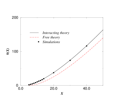
Figure 1: Persistence exponent $\theta$ as a function of the threshold $X$ for the process $\xi(t)$ of Eq. (72) with $a=1,\,\rho=10,$ and $\beta=2$. The average value of this process is $\langle\xi\rangle=5.$ The error bars of the simulation data are smaller than the symbols. The interacting theory expanded to leading order (solid line, Eq. (8) of this work) is in excellent agreement with the simulations.

Figure 2: Same as Fig. 1, zoomed on thresholds $X$ close above the average $\langle\xi\rangle=5$.

Fig. 2 shows a zoom on values $X\>\raisebox{-2.15277pt}{$\stackrel{{\scriptstyle\textstyle>}}{{\sim}}$}\>\langle\xi\rangle$; the leading order behavior of the interacting theory (solid curve) still represents a considerable improvement over the free theory, but as $X\to\langle\xi\rangle$, higher orders in the expansion become necessary. For $X<\langle\xi\rangle$ the expansion of this work does not apply.

Second example.   Let $A(\xi)$ be such that for some small parameter $\epsilon$

$$A(\xi)={\cal A}(\epsilon\xi)$$ (75)

Eq. (10) may then be recast in the form

$$\epsilon t=-\int_{\epsilon X}^{\epsilon f(t)}\frac{\mbox{d}x}{{\cal A}(x)}$$ (76)

whence it follows that $f(t)$ scales as

$$f(t)=\epsilon^{-1}{\cal F}(\epsilon t;\epsilon X)$$ (77)

We have by construction $f(0)=X$ as before. Furthermore

$$f^{(n)}(0)=\epsilon^{k-1}{\cal F}^{(k)}(0;\epsilon X)$$ (78)

where the differentiations of ${\cal F}$ are with respect to its first argument. If now we agree to choose $X$ of order $\epsilon^{-1}$, then the $k$th derivative of $f$ is of order $\epsilon^{k-1}$. This guarantees that $g_{k}$ is of order $\epsilon^{k}$, as is illustrated by Eqs. (27) for $g_{1}$ and $g_{2}$. Hence the conditions of limit (i) are fulfilled and the calculation of Subsection 4.4 applies.

In order to test the nonanalytic dependence on the curvature parameter $g$ in Eq. (68) we have performed a Monte Carlo simulation of $\xi(t)$ for the particular choice

$$f(t)=X-\beta t+\epsilon t^{2}$$ (79)

that is,  ${\cal F}(x,y)=x-\beta y+y^{2}$. The corresponding $\cal{A}$ follows from Eq. (76) and by means of Eqs. (75) and (5) we find

$$g=1-\Big{(}1+\frac{4\epsilon a}{\beta^{2}}\Big{)}^{-1/2}$$ (80)

Monte Carlo simulations were carried out at fixed $a$ and $\beta$ for various values of $\epsilon.$ In Fig. 3 we show the persistence exponent $\theta$ as a function of $g$, together with the theoretical $g^{2/3}$ law of Eq. (68). The agreement is excellent.

Figure 3: Persistence exponent $\theta$ for fixed threshold $X$ as a function of the curvature parameter $g$ for the second example of Section 5 with $a=1,\,\rho=10,$ and $\beta=20.$ The solid line represents the theoretical $g^{2/3}$ law (Eq. (68) of this work), which appears to provide an excellent description of the data.

6 Limit of Gaussian noise

The Langevin equation (with white Gaussian noise) and its extension to colored Gaussian noise are at the basis of much recent work on persistence; see e.g. the recent review by Majumdar [2]. There is a large body of knowledge today about the persistence properties of such Gaussian Markovian processes, and a perturbative method around the Markovian case has recently been devised by Majumdar and Sire [4] (see also Oerding et al. [5] and Majumdar et al. [6]). The equation of this work, Eq. (1), with jumps of arbitrary finite size $a$, provides, on the contrary, an example of strongly non-Gaussian noise. In this section we show how for $a\to 0$ the Gaussian limit is approached. This limit, just as the one of zero curvature considered in Section 3, is a singular point in parameter space.

6.1 Gaussian persistence exponent $\theta_{G}$

Let $\zeta(t)$ obey the linear Langevin equation

$$\frac{\mbox{d}\zeta}{\mbox{d}t}=-\beta\zeta+L(t)$$ (81)

where $L(t)$ is Gaussian white noise of average $\langle L(t)\rangle=0$ and correlation

$$\langle\zeta(t)\zeta(t^{\prime})\rangle=\Gamma\delta(t-t^{\prime})$$ (82)

The level exponent $\theta_{G}(Z)$ for this process, associated with the probability for $\zeta(t)$ not to have crossed a preestablished threshold $\zeta=Z$ in a time interval has not to our knowledge been calculated in the literature. The related exponent associated with crossing upward through the threshold has been considered by Krapivsky and Redner [13] (see also Turban [14]). It is easy to find $\theta_{G}(Z)$ by a method similar to theirs, as we will show now. The probability distribution $P(\zeta,t)$ for the process (81) evolves in time [18] according to the Fokker–Planck equation

$$\frac{\partial P}{\partial t}=\beta\frac{\partial}{\partial\zeta}\zeta P+\frac{\Gamma}{2}\frac{\partial^{2}}{\partial\zeta^{2}}P$$ (83)

The persistence exponent $\theta_{G}$ is the eigenvalue of the slowest decaying mode for $Z\!<\!\zeta\!<\!\infty$ satisfing the boundary condition $P(Z,t)=0$. We set $P(\zeta,t)=P(\zeta)\exp(-\theta_{G}\,t)$. It is well-known that the equation for $P(\zeta)$ can be transformed to the eigenvalue equation for the quantum harmonic oscillator. This fact has been exploited in previous work [4, 6, 13] on persistence exponents. Here, in view of our interest in the interval $Z<\zeta<\infty$ and the limit of large $Z$, we must transform

$$\tilde{P}(\mathaccent 126{\zeta})=\mbox{e}^{\frac{\beta}{2\Gamma}\zeta^{2}}P(\zeta)$$ (84)

with $\mathaccent 126{\zeta}=\lambda^{1/6}(\sqrt{2\beta/\Gamma}\,\zeta-2\sqrt{\lambda})$ and $\lambda=1/2+\theta_{G}/\beta$. Then $\tilde{P}(\mathaccent 126{\zeta})$ satisfies the eigenvalue problem

$$\left(\frac{\mbox{d}^{2}}{\mbox{d}\mathaccent 126{\zeta}^{2}}-\mathaccent 126{\zeta}\left(1+\frac{1}{4}\mathaccent 126{\zeta}\lambda^{-2/3}\right)\right)\tilde{P}(\mathaccent 126{\zeta})=0,\qquad\tilde{P}(\mathaccent 126{Z})=0$$ (85)

In the limit of high threshold $Z$ we expect $\theta_{G}$, and therefore $\lambda$, to diverge. Hence in this limit

$$\left(\frac{\mbox{d}^{2}}{\mbox{d}\mathaccent 126{\zeta}^{2}}-\mathaccent 126{\zeta}\right)\tilde{P}(\mathaccent 126{\zeta})=0,\qquad\tilde{P}(\mathaccent 126{Z})=0$$ (86)

The solution of Eq. (86) that vanishes for $\mathaccent 126{\zeta}\to\infty$ is the Airy function $\mbox{Ai}(\mathaccent 126{\zeta})$. The boundary condition $\mbox{Ai}(\mathaccent 126{Z})=0$ leads to $\mathaccent 126{Z}=a_{1}$, where $a_{1}=-2.3381$…  is the first zero of Ai. This condition fixes $\theta_{G}$ in terms of $Z$; upon expanding for large $Z$ one finds

$$\theta_{G}(Z)=\frac{\beta^{2}Z^{2}}{2\Gamma}+|a_{1}|\beta^{{\frac{2}{3}}}{\left(\frac{\beta^{2}Z^{2}}{2\Gamma}\right)}^{\frac{1}{3}}+\ldots\qquad(Z\to\infty)$$ (87)

which is the desired result.

6.2 Gaussian limit

6.2.1 Limiting procedure

In Eq. (1) we substitute now $\xi=\zeta+\rho a/\beta$ and $a\sum_{k}\delta(t-t_{k})-\rho a=L(t)$ and take the ”Gaussian” limit, defined as

$$\rho\to\infty,\quad a\to 0\qquad\mbox{with }\Gamma=\rho a^{2}\mbox{ fixed}$$ (88)

The result is that Eq. (81) appears. One easily verifies that $\langle L(t)\rangle=0$ and that the cumulants of $L$, which for $n=2,3,\ldots$ are given by

$$\langle L(t_{1})\ldots L(t_{n})\rangle_{c}=\rho a^{n}\prod_{k=1}^{n-1}\delta(t_{k}-t_{k+1})$$ (89)

vanish in the limit of Eq. (88) when $n\geq 3$. Hence $L(t)$ is Gaussian white noise. The above transformation changes the threshold $X$ into $Z=X-\rho a/\beta$. One now expects that the Gaussian persistence exponent $\theta_{G}(Z)$, found by direct calculation at the end of the previous subsection, should also be accessible as a limiting case of our general approach. Naively, one may attempt to obtain $\theta_{G}(Z)$ by taking the Gaussian limit, followed by the limit $Z\to\infty$, in expression (68) for $\theta$. After a short calculation that procedure leads to

$$\theta_{G}(Z)=\frac{\beta^{2}Z^{2}}{2\Gamma}+{\left(\frac{9\pi}{8}\right)}^{\frac{2}{3}}\beta^{{\frac{2}{3}}}{\left(\frac{\beta^{2}Z^{2}}{2\Gamma}\right)}^{\frac{1}{3}}+\ldots\qquad(Z\to\infty)$$ (90)

This differs from the exact result, Eq. (87), only by the numerical value of the coefficient of the subleading term; moreover, the difference ($(9\pi/8)^{2/3}\simeq 2.3203\ldots$ versus $|a_{1}|=2.3381\ldots$) is only about one percent! Nevertheless, Eq. (87) is right and (90) is not. The rather obvious reason is that the Gaussian limit (which implies $aZ\to 0$), followed by $Z\to\infty$, does not commute with the limit that was taken to arrive at Eq. (68) (viz. $r,g\to 0$ at fixed $r/g$, which implies $aZ\to\infty$). In order to find $\theta_{G}(Z)$ within the formalism of the preceding sections it is necessary to start again from the integral representation of $H(\Omega;r,g)$ in Eq. (56). Below we will see how to do that.

6.2.2 Calculation of $\,\theta_{G}$

Let us consider $H(\Omega;r,g)$ of Eq. (56). In view of Eqs. (57)-(59) it is represented as an integral on $\nu$ of the function $\exp({g^{-1}h(\nu,\Omega)})$. The Gaussian limit is controlled by the parameter $a$, which should tend to zero. At fixed $\Gamma=\rho a^{2}$ and $Z=X-\rho a/\beta$ we find from Eq. (73) that in that limit $g=\gamma a^{2}+{\cal O}(a^{3})$ and $r=1-a\gamma Z+{\cal O}(a^{2})$ with $\gamma=\beta/\Gamma$. We recall now Eq. (21), which says that $\theta=\rho(1-\Omega_{1})$. Expecting $\theta$ to approach a finite limit $\theta_{G}$, we set $\Omega=1-a^{2}W$, where $W$ is the appropriately scaled variable for the relevant region of the complex frequency plane. Hence, if the rightmost zero of $H(\Omega;r,g)$ in this plane occurs for $W=W_{1}$, then

$$\theta_{G}=\lim_{a\to 0}\,\rho(1-\Omega_{1})=\Gamma W_{1}$$ (91)

Stationary points. As a preliminary we consider the stationary points of $h(\nu,\Omega)$. Expanding the equation $\partial h/\partial\nu=0$ for small $a$ while anticipating that $\mbox{e}^{\nu}$ will be small we find that these points are solutions of

$$-a^{2}W+(1-a\gamma Z)\mbox{e}^{\nu}-\mbox{e}^{\nu}-\frac{1}{2}\mbox{e}^{2\nu}+\ldots=0$$ (92)

where the dots represent terms of higher order in $a$ and $\mbox{e}^{\nu}$. This shows that there exist solutions with the scaling $\mbox{Re}\,\nu_{\pm}\sim\log a$ for $a\to 0$. Solving explicitly we obtain

$$\mbox{e}^{\nu_{\pm}}=a\,\gamma Z\left(-1\pm\sqrt{1-\frac{2W}{\gamma^{2}Z^{2}}}\right)+{\cal O}(a^{2})$$ (93)

In the above expression there appears a critical value of $W$ equal to $W_{c}=\frac{1}{2}\gamma^{2}Z^{2}$. For $W\!>\!W_{c}$, which we expect to be the relevant regime, the stationary points therefore are $\nu_{\pm}=-A-\mbox{i}\pi\pm\mbox{i}\mu^{*}$ with

$$-A=\log(a\sqrt{2W})+{\cal O}(a\log a),\qquad\mu^{*}=\arccos\frac{\gamma Z}{\sqrt{2W}}+{\cal O}(a)$$ (94)

Instead of the variable of integration $\nu$ we will henceforth use $\mu$ defined by

$$\nu=-A-\mbox{i}\pi+\mbox{i}\mu$$ (95)

We will not exploit directly, in what follows, our knowledge of $\mu^{*}$.

Gaussian limit. We consider $h(\nu,\Omega)$ of Eq. (59) as a function of $\mu$. After some calculation we find that for small $a$

$$h(\nu,\Omega)=h(-A-\mbox{i}\pi,\Omega)+a^{2}\gamma k(\mu,W)+{\cal O}(a^{3})$$ (96)

with

$$\gamma k(\mu,W)=-\mbox{i}W\mu+\gamma Z\sqrt{2W}(\mbox{e}^{\mbox{i}\mu}-1)-\frac{1}{2}W(\mbox{e}^{2\mbox{i}\mu}-1)$$ (97)

In the limit $a\to 0$ the function $H(\Omega;r,g)$ may therefore be rewritten as the integral

$$H(\Omega;r,g)=D\int\mbox{d}\mu\,\,\mbox{e}^{k(\mu,W)}$$ (98)

with $k(\mu,W)$ given by Eq. (97) and where $D$ diverges when $a$ goes to zero. However, $D$ will divide out in Eq. (50) against the same factor in the numerator of $K(\Omega)$. This completes the Gaussian limit. There is no small parameter left in the integral in Eq. (98).

Limit of large $Z$. This integral may be reduced to a more elementary one in the limit of large threshold $Z$. The reason is that then the relevant values of $W$ are close to $W_{c}$. We adopt the scaling

$$W\,=\,W_{c}(1+wZ^{-4/3})\,=\,\frac{1}{2}\gamma^{2}Z^{2}(1+wZ^{-4/3})$$ (99)

which will be justified by the results. We now consider the full Taylor series in $\mu$ of $k(\mu,W)$. Upon expanding each of its coefficients for large $Z$ and retaining only the leading term we get

$$k(\mu,W) = -\frac{1}{2}\gamma wZ^{2/3}\mbox{i}\mu-\frac{1}{2}\gamma wZ^{2/3}\frac{(\mbox{i}\mu)^{2}}{2!}$$ (100)

$$-\gamma Z^{2}\,\sum_{n=3}^{\infty}(2^{n-2}-1)\frac{(\mbox{i}\mu)^{n}}{n!}$$

If now the integration variable is scaled according to $\mu=\lambda(\gamma Z^{2})^{-1/3}$, then in the large $Z$ limit all terms in Eq. (100) except those with $n=1$ and $n=3$ go to zero. We are left with

$$H(\Omega;r,g)\,\sim\,\int\mbox{d}\lambda\,\,\mbox{e}^{-\frac{1}{2}\gamma^{2/3}w\,\mbox{\small i}\lambda+\frac{1}{6}\mbox{\small i}\lambda^{3}}\qquad(a=0;\,Z\to\infty)$$ (101)

which is the integral representation of the Airy function. The only dependence left is on the variable $w$. Let the rightmost zero of $H(\Omega;r,g)$ in the complex frequency plane occur for $w=w_{1}$. We see now that $w_{1}$ is the solution of $\mbox{Ai}(\gamma^{2/3}w_{1})=0$, whence

$$w_{1}=|a_{1}|\left(2\Gamma/\beta\right)^{2/3}$$ (102)

Upon relating $w_{1}$ to $W_{1}$ by Eq. (99) and using Eq. (91) we finally get the expression of Eq. (87) for $\theta_{G}$.

Discussion.   It is instructive to return to the quantity $\mu^{*}$ given by Eq. (94). The two stationary points are separated by a distance $2\mu^{*}$, and substituting the various scaling transformations we see that, as $Z\to\infty$, they have in terms of $\lambda$ the finite distance $2\lambda^{*}=2\gamma^{1/3}w^{1/2}$. We now observe the mechanism that is at work here. In Section 4, for $a$ finite, hence far from the Gaussian limit, $H(\Omega;r,g)$ is the sum of contributions from two stationary points at infinite separation ($\sim g^{-1}$ with $g\to 0$) in the $\nu$ plane; as the Gaussian limit is approached, the two stationary points come within finite distance of one another, and their contributions cannot be separated any longer. This ”interaction” between the stationary points leads to the replacement of the cosine in Eq. (66) by the Airy function in Eq. (101), and finally affects by about one percent the coefficient of the subleading term of the persistence exponent.

7 Conclusion

Beside many Gaussian persistence problems, there are also non-Gaussian ones occurring in statistical physics. We have pointed out and studied one class of such problems, associated with the specific non-Gaussian stochastic process that satisfies Eq. (1). Its relation to several questions in statistical physics has been indicated in the Introduction. The sample functions of this process are deterministic curves interrupted at random instants of time by upward jumps. Among these, a zeroth order subclass is constituted by ”random sawtooth” functions, characterized by linear decay with fixed slope. The persistence exponent $\theta_{0}$ of this subclass is easy to find. We then perturb around this zeroth order problem by introducing in the decay a small curvature of strength controlled by a parameter $g$. As a consequence we have to deal with what is essentially a one-dimensional interacting particle system with coupling constant $g$, and the mathematics becomes considerably more complicated. The case of greatest importance covered by the present work is the linear equation, with exponential decay curve, that prevails for $A(\xi)=\beta\xi$ in Eq. (1). Our result for this case is an asymptotic expansion, Eq. (8), of the persistence exponent $\theta(X)$ in the limit of high threshold $X$.

The same equation for level $X=\langle\xi(t)\rangle$, which is outside of the domain of the asymptotic expansion of this work, has recently been considered by Deloubrière [12]. It would be of definite interest to extend Eq. (1) to random upward jumps $a_{k}$ at time $t_{k}$, given that specific distributions of jump sizes $a_{k}$ naturally occur in several models of statistical physics [10, 11].

Appendix A A theorem by Takács

We consider the problem of determining the probability $p_{L}$ that occurs Section 3. Let the variables $M_{k}$ be those defined there. It is natural to set in addition $M_{0}=0$ and $M_{L+1}=L$, so that our problem is to find

$$p_{L}\,=\,\mbox{Prob}\,\{k-M_{k}>0\mbox{ \,for\, }k=1,\ldots,L+1\}$$ (103)

Relevant to this problem is Theorem 3 by Takács [19], which concerns nondecreasing random functions on line segments. The author [19] indicates that this theorem has an analog valid for nondecreasing random sequences. For the present case the full proof runs as follows.

The range of the index $k$ may be extended to arbitrary positive $k$ by the definition

$$M_{L+1+k}=L+M_{k}$$ (104)

This amounts to repeating the set of random point on $0<s\leq L+1$ periodically in the segments  $n(L+1)<s\leq(n+1)(L+1)$,  where $n=1,2,\ldots.$ The random variable $M_{k+\ell}-M_{k}$, where $k=0,1,2,\ldots$ and $\ell=1,2,\ldots,$ represents the number of points in the interval $k<s\leq k+\ell$, and the probability distribution of this variable is obviously independent of $k$. Let now for $k=0,1,2,\ldots$

$$\delta_{k}=\left\{\begin{array}[]{ll}1&\mbox{ if\, }M_{k+\ell}-M_{k}<\ell\mbox{ \,for\, }\ell=1,2,\ldots\\[5.69054pt] 0\phantom{xx}&\mbox{ otherwise}\end{array}\right.$$ (105)

Then the probability distribution of $\delta_{k}$ does not depend on $k$, and $\delta_{k+L+1}=\delta_{k}$. It is easy to verify that $M_{k+\ell}-M_{k}<\ell$ holds for all $\ell$ if it holds for $\ell=1,2,\ldots,L+1$. Hence Eq. (103) shows that $p_{L}$ is the probability that $\delta_{0}$ be equal to 1. We may write equivalently $p_{L}=\langle\delta_{0}\rangle$, where the average is on all random sequences $M_{1},\ldots,M_{L}$. But since all $\delta_{k}$ have the same distribution, hence the same average, we also have

$$p_{L}\,=\,\frac{1}{L+1}\sum_{k=1}^{L+1}\langle\delta_{k}\rangle\,=\,\frac{1}{L+1}\,\langle\sum_{k=1}^{L+1}\delta_{k}\rangle$$ (106)

We consider now the sum on the $\delta_{k}$ in the last member of the above equation. The condition for $\delta_{k}$ to equal 1 may be rewritten as

$$j-M_{j}>k-M_{k}\quad\mbox{ for all\, }j=k+1,\ldots,k+L+1$$ (107)

In the range $k\leq j\leq k+L+1$ the function $j-M_{j}$ has the initial value $k-M_{k}$ and the final value $k+L+1-M_{k+L+1}=k-M_{k}+1$, where we used the definition (104). If $\delta_{k}=1$, then $j-M_{j}\geq k-M_{k}+1$ for all $j=k+1,\ldots,k+L+1$, and this means that $\delta_{k+1}=\ldots=\delta_{k+L}=0$. Hence $\sum_{j=k}^{k+L}\delta_{j}$ can be equal only to 0 or to 1. We now prove that in fact it equals unity. For it to be zero, all $\delta_{j}$ in the range of summation would have to vanish, whence we would have $\delta_{j}=0$ for all $j\geq k$. There would then exist an increasing sequence $\{j_{r}\}_{r=0}^{\infty}$ (where $j_{0}=k$) such that the corresponding sequence $\{j_{r}-M_{j_{r}}\}_{r=0}^{\infty}$ is nonincreasing. This however is in contradiction with the fact that $j-M_{j}$ increases by $1$ whenever $j$ is augmented by $L+1$. It follows that $\sum_{j=k}^{k+L}\delta_{k}=1$,  whence by Eq. (106) we obtain $p_{L}=1/(L+1)$ and $I_{L}=(L+1)^{L-1}/L!$

References

- [1] I. F. Blake and W. C. Lindsay, IEEE Trans. Info. Theory 19 (1973) 295.
- [2] S.N. Majumdar, cond-mat/9907407.
- [3] C. Godrèche, in: Self-Similar Systems, V.B. Priezzhev and V.P. Spiridonov eds. (JINR, Dubna 1999).
- [4] S. N. Majumdar and C. Sire, Phys. Rev. Lett. 77 (1996) 1420.
- [5] K. Oerding, S.J. Cornell, and A.J. Bray, Phys. Rev. E 56 (1997) R25.
- [6] C. Sire, S. N. Majumdar, and A. Rüdinger, cond-mat/9810136.
- [7] S. N. Majumdar and A.J. Bray, Phys. Rev. Lett. 81 (1998) 2626.
- [8] S. N. Majumdar, C. Sire, A. J. Bray, and S. J. Cornell, Phys. Rev. Lett. 77 (1996) 2867.
- [9] B. Derrida, V. Hakim, and R. Zeitak, Phys. Rev. Lett. 77 (1996) 2871.
- [10] S. R. Gomes Júnior, O. Deloubrière, and H.J. Hilhorst, in preparation.
- [11] J.E. de Freitas and L. dos Santos Lucena, Physica A 266 (1999) 81.
- [12] O. Deloubrière, in preparation.
- [13] P. L. Krapivsky and L. Redner, Am. J. of Phys. 64 (1996) 564.
- [14] L. Turban, J. Phys. A 25 (1992) L127.
- [15] I. Dornic and C. Godrèche, J. Phys. A 31 (1998) 5413.
- [16] M. Bauer, C. Godrèche, and J.-M. Luck, cond-mat/9905252.
- [17] G. Gasper and M. Rahman, Basic Hypergeometric Series, (Cambridge University Press, Cambridge 1990).
- [18] N. G. van Kampen, Stochastic Processes in Physics and Chemistry (North-Holland, Amsterdam 1992).
- [19] L. Takács, in: Proc. Fifth Berkeley Symp. on Math. Stat. and Prob., Vol. II, L.M. Le Cam and J. Neyman, eds., Part I, p. 431 (Univ. California Press, Berkeley 1967).