Correlated Electrons in Carbon Nanotubes

Abstract

Single-wall carbon nanotubes are almost ideal systems for the investigation of exotic many-body effects due to non-Fermi liquid behavior of interacting electrons in one dimension. Recent theoretical and experimental results are reviewed with a focus on electron correlations. Starting from a microscopic lattice model we derive an effective phase Hamiltonian for conducting single-wall nanotubes with arbitrary chirality. The parameters of the Hamiltonian show very weak dependence on the chiral angle, which makes the low-energy physics of conducting nanotubes universal. The temperature-dependent resistivity and frequency-dependent optical conductivity of nanotubes with impurities are evaluated within the Luttinger-like model. Localization effects are studied. In particular, we found that intra-valley and inter-valley electron scattering can not coexist at low energies. Low-energy properties of clean nanotubes are studied beyond the Luttinger liquid approximation. The strongest Mott-like electron instability occurs at half filling. In the Mott insulating phase electrons at different atomic sublattices form characteristic bound states. The energy gaps of $0.01-0.1$ eV occur in all modes of elementary excitations. We finally discuss observability of the Mott insulating phase in transport experiments. The accent is made on the charge transfer from external electrodes which results in a deviation of the electron density from half-filling.

1 Introduction

Single-wall carbon nanotubes (SWNTs) are cylindrical fullerene structures with diameters in the nanometer range and lengths of few micrometers DekkerRev . Experimental demonstration of electron transport through SWNTs Tans ; Bockrath has been followed by observations of atomic structure Wildoer ; Odom ; Johnson , one-dimensional van Hove singularities Wildoer ; Odom , standing electron waves Venema and electron correlations BockrathLL ; SchonenbergerLL ; Yao in these systems. Moreover, first prototypes of SWNT functional devices - diodes Yao ; Fuhrer and field effect transistors Tans3 - have been demonstrated recently.

On one hand, SWNTs can be viewed as giant macromolecules whose properties can be learned from the first principle calculations. On the other hand, SWNTs are perfect one-dimensional (1D) model systems to be studied by methods of the solid state theory. This somewhat reductionist but insightful approach provides a reasonable description for the bulk of experimental data obtained up to date.

On a single-particle level physical properties of SWNTs are determined by their geometry. Depending on the wrapping vector, SWNTs can either be 1D metals or semiconductors with the energy gap in sub-electronvolt range. This has been confirmed by direct observation of 1D van Hove singularities in scanning tunneling microscopy experiments Wildoer ; Odom .

In this paper we address the role of the Coulomb interaction in 1D SWNTs and review recent results on electron correlation effects. Away from half-filling electron correlations are well described by Luttinger-like models KBF ; Egger-Gogolin ; YOprl99 . In particular, the non-Fermi liquid ground state of the system is characterized by a power-law suppression of the density of electronic states near the Fermi level. This effect has been observed in single- BockrathLL and, presumably, multi-wall SchonenbergerLL nanotubes, as well as in junctions between metallic SWNTs Yao . Transport properties of metallic nanotubes with impurities are affected by the Coulomb interaction as well Yoshioka-impurities .

The low-energy properties of SWNTs are different at half-filling due to the umklapp scattering. The latter is coupled to the strongly interacting total charge mode. This makes the umklapp scattering a strongly relevant perturbation. As a result, the Mott-like electron instability occurs in the electronic spectrum of SWNTs and energy gaps open in all modes of the elementary excitations KBF ; YOprl99 . The transition to the Mott insulating phase should manifest itself by an increased resistivity of half-filled SWNTs at low temperatures.

The plan of the paper is as follows. In Section 2 we derive an effective low-energy model for metallic SWNTs with arbitrary chirality, which naturally includes one-electron backscattering on impurities as well as two-electron umklapp scattering at half-filling. We discuss the non-Fermi liquid properties of clean SWNTs within the Luttinger-like model in Section 3 and evaluate electron transport in SWNTs with impurities in Section 4. The effect of interactions beyond the Luttinger model is analyzed within the renormalization group scheme in Section 5. The Mott-like electron instability is further investigated in Section 6 using the self-consistent harmonic approximation. Finally, we discuss observability of the Mott-insulating phase in experiments (Section 7).

2 Universal Model of Metallic Nanotubes

2.1 Microscopic theory

Structurally uniform SWNTs can be characterized by the wrapping vector $\vec{w}=N_{+}\vec{a}_{+}+N_{-}\vec{a}_{-}$ given by the linear combination of primitive lattice vectors $\vec{a}_{\pm}=(\pm 1,\sqrt{3})a/2$, with $a\approx 0.246$ nm (Fig. 1). It is natural to separate non-chiral armchair ($N_{+}=N_{-}$) and zig-zag ($N_{+}=-N_{-}$) nanotubes from their chiral counterparts. Recent scanning tunneling microscopy studies Wildoer ; Odom have revealed that individual SWNTs are generally chiral. According to the single-particle model, the nanotubes with $N_{+}-N_{-}=0$ mod $3$ have gapless energy spectrum and are therefore conducting; otherwise, the energy spectrum is gapped and SWNTs are insulating.

We consider metallic SWNT whose axis $x^{\prime}$ forms an angle $\chi=\arctan[(N_{-}-N_{+})/\sqrt{3}(N_{+}+N_{-})]$ with the direction of the chains of carbon atoms ($x$ axis in Fig. 1). We expand the standard single-particle Hamiltonian Wallace $H_{k}$ for electrons on two atomic sublattices $p=\pm$ of a graphite sheet (Fig. 1) near the Fermi points $\alpha\vec{K}$ (with the valley index $\alpha=\pm$, and $\vec{K}=(4\pi/3a,0)$) to the lowest order in $\vec{q}=\vec{k}-\alpha\vec{K}=q(\cos\chi,\sin\chi)$. Introducing slowly varying Fermi fields $\psi_{p\alpha s}(x^{\prime})=L^{-1/2}\sum_{q=2\pi n/L}e^{iqx^{\prime}}a_{p\alpha s}(\vec{q}+\alpha\vec{K})$, we obtain,

$$H_{k}=-iv\sum_{p\alpha s}\alpha e^{-ip\alpha\chi}\int\mathrm{d}x^{\prime}\psi_{p\alpha s}^{\dagger}\partial_{x^{\prime}}\psi_{-p\alpha s},$$ (1)

where $v\approx 8.1\times 10^{5}$ m/s is the Fermi velocity, and $s=\pm$ is the electron spin.

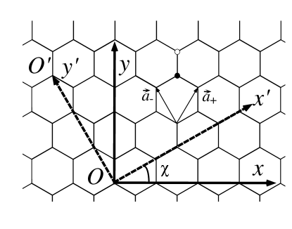
Figure 1: Graphite lattice consists of two atomic sublattices $p=+,-$ denoted by filled and open circles. SWNT at the angle $\chi$ to $x$ axis can be formed by wrapping the graphite sheet along $\vec{w}=OO^{\prime}$ vector.

The kinetic term can be diagonalized by the unitary transformation

$$\psi_{p\alpha s}=\frac{1}{\sqrt{2}}e^{-ip\alpha\chi/2}\sum_{r=\pm}(r\alpha)^{\frac{1-p}{2}}\varphi_{r\alpha s}$$ (2)

to the basis $\varphi_{r\alpha s}$ of right- ($r=+$) and left- ($r=-$) and moving electrons.

The Coulomb interaction has the form

$$H_{int}=\frac{1}{2}\sum_{pp^{\prime},\left\{\alpha_{i}\right\},ss^{\prime}}V_{pp^{\prime}}(2\bar{\alpha}K)\int dx^{\prime}\psi_{p\alpha_{1}s}^{\dagger}\psi_{p^{\prime}\alpha_{2}s^{\prime}}^{\dagger}\psi_{p^{\prime}\alpha_{3}s^{\prime}}\psi_{p\alpha_{4}s},$$ (3)

with the matrix elements $V_{pp^{\prime}}(2\bar{\alpha}K)$ corresponding to the amplitudes of intra- ($p=p^{\prime}$) and inter- ($p=-p^{\prime}$) sublattice intra- ($\bar{\alpha}=0$) and inter- ($\bar{\alpha}=\pm 1$) valley scattering (here $\bar{\alpha}=(\alpha_{1}-\alpha_{4})/2=(\alpha_{3}-\alpha_{2})/2$). In Eq. (3) we assume that the fields $\psi$ are varying slowly on the scale of the screening radius $R_{s}$ of the Coulomb interaction determined by the distance to a gate electrode. This corresponds to a contact-interaction approximation. Equation (3) is therefore valid at large length scale $x^{\prime}\gg R_{s}$ and low electron energy $E\ll\hbar v/R_{s}$.

The dominant contribution to the intra-valley scattering amplitudes $V_{pp^{\prime}}(0)$ comes from the long range component of the Coulomb interaction, $V_{pp}(0)\simeq V_{p-p}(0)\simeq e^{2}/C\simeq(2e^{2}/\kappa)\ln(R_{s}/R)$, $C$ being the capacitance of SWNT per unit length KBF . The differential part $\Delta V(0)=V_{pp}(0)-V_{p-p}(0)$ of intra-valley scattering as well as the intra-sublattice inter-valley $V_{pp}(2K)$ are estimated at $\Delta V(0),V_{pp}(2K)$ $\sim ae^{2}/\kappa R$ . Despite $\Delta V(0),V_{pp}(2K)$ being much smaller than $V_{pp}(0),$ they cause non-Luttinger terms in the low-energy Hamiltonian which will be important in the further analysis. The matrix elements $V_{pp^{\prime}}(2\bar{\alpha}K)$ have been evaluated numerically for all SWNTs with radii $R$ in the range $2R/a=4-7$ ($2R/a=5.5$ for (10,10) SWNTs). We found that dimensionless amplitudes $2\pi\kappa R[\Delta V(0),V_{pp}(2K)]/ae^{2}$ show very weak dependence on the radius of SWNT and its chiral angle (see Table 1). The results are sensitive to the value the short distance cutoff $a_{0}\sim a$ of the Coulomb interaction.

Table 1: Scattering amplitudes $\Delta V(0)$, $V_{pp}(2K)$, $V_{p-p}(2K)$ in units $ae^{2}/2\pi\kappa R$ for all SWNTs with $2R/a=4-7$. The cutoff parameter $a_{0}=0.526a$ is obtained from the requirement that the on-site interaction in the original tight-binding model is equal to the difference between the ionization potential and electron affinity of $sp^{2}$ hybridized carbon Moore .

$a_{0}/a$	$\Delta V(0)$	$V_{pp}(2K)$	$|V_{p-p}(2K)|$
$0.4$	$0.44265-0.44274$	$0.97060-0.97095$	$0.6-2.2\times 10^{-3}$
$0.526$	$0.17378-0.17395$	$0.53549-0.53561$	$0.5-1.6\times 10^{-3}$
$0.7$	$0.04880-0.04895$	$0.24778-0.24797$	$0.3-1.5\times 10^{-3}$

The inter-sublattice inter-valley scattering amplitude $V_{p-p}(2K)$ is almost three orders of magnitude smaller than $\Delta V(0)$, $V_{pp}(2K)$. This is due to the $C_{3}$ symmetry of a graphite lattice ($V_{p-p}(2K)=0$ for a plane graphite sheet). The matrix elements $V_{p-p}(2K)$ are generally complex due to the asymmetry of effective 1D inter-sublattice interaction potential (the matrix elements are real for symmetric zig-zag and armchair SWNTs). Let us note that after the unitary transformation (2) of the Hamiltonian $H=H_{k}+H_{int}$, the chiral angle $\chi$ enters only into the inter-sublattice inter-valley scattering matrix elements $V_{p-p}(2K)$. Due to the smallness of these matrix elements, the low-energy properties of chiral SWNTs are expected to be virtually independent of the chiral angle.

2.2 Bosonization

The transformed Hamiltonian $H$ can be bosonized by introducing the phase representation of the Fermi fields Egger-Gogolin ; YOprl99 ,

$$\varphi_{r\alpha s}=\frac{\eta_{r\alpha s}}{\sqrt{2\pi\tilde{a}}}\exp\left[\mathrm{i}rq_{F}x^{\prime}+\frac{\mathrm{i}r}{2}\left\{\theta_{\alpha s}+r\phi_{\alpha s}\right\}\right].$$ (4)

The phase variables $\theta_{\alpha s},\phi_{\alpha s}$  are further decomposed into symmetric $\delta=+$ and antisymmetric $\delta=-$ modes of the charge $\rho$ and spin $\sigma$ excitations, $O_{\alpha s}=O_{\rho+}+sO_{\sigma+}+\alpha O_{\rho-}+\alpha sO_{\sigma-}$, $O=\theta,\phi$. The bosonic fields satisfy the commutation relation, $[\theta_{j\delta}(x_{1}),\phi_{j^{\prime}\delta^{\prime}}(x_{2})]=\mathrm{i}(\pi/2)\mathrm{sign}(x_{1}-x_{2})\delta_{jj^{\prime}}\delta_{\delta\delta^{\prime}}$. The Majorana fermions $\eta_{r\alpha s}$ are introduced to ensure correct anticommutation rules for different species $r,\alpha,s$ of electrons, and satisfy $[\eta_{r\alpha s},\eta_{r^{\prime}\alpha^{\prime}s^{\prime}}]_{+}=2\delta_{rr^{\prime}}\delta_{\alpha\alpha^{\prime}}\delta_{ss^{\prime}}$. The quantity $q_{F}=\pi n/4$ is related to the deviation $n$ of the average electron density from half-filling, and $\tilde{a}\sim a$ is the parameter of the exponential ultraviolet cutoff.

Neglecting the inter-sublattice inter-valley scattering we arrive at the universal phase Hamiltonian of metallic SWNTs,

$$H = \sum_{j=\rho,\sigma}\sum_{\delta=\pm}\frac{v_{j\delta}}{2\pi}\int\mathrm{d}x^{\prime}\left\{K_{j\delta}^{-1}(\partial_{x^{\prime}}\theta_{j\delta})^{2}+K_{j\delta}(\partial_{x^{\prime}}\phi_{j\delta})^{2}\right\}+\frac{1}{2(\pi\tilde{a})^{2}}\int\mathrm{d}x^{\prime}$$ (10)

$$\{[\Delta V(0)-V_{pp}(2K)][\cos(4q_{F}x^{\prime}+2\theta_{\rho+})\cos 2\theta_{\sigma+}-\cos 2\theta_{\rho-}\cos 2\theta_{\sigma-}]$$

$$-\Delta V(0)\cos(4q_{F}x^{\prime}+2\theta_{\rho+})\cos 2\theta_{\rho-}+\Delta V(0)\cos(4q_{F}x^{\prime}+2\theta_{\rho+})\cos 2\theta_{\sigma-}$$

$$-{\Delta V(0)}\cos 2\theta_{\sigma+}\cos 2\theta_{\rho-}+{\Delta V(0)}\cos 2\theta_{\sigma+}\cos 2\theta_{\sigma-}$$

$$-{V}_{pp}{(2K)}\cos(4q_{F}x^{\prime}+2\theta_{\rho+})\cos 2\phi_{\sigma-}+{V}_{pp}{(2K)}\cos 2\theta_{\sigma+}\cos 2\phi_{\sigma-}$$

$$+{V}_{pp}{(2K)}\cos 2\theta_{\rho-}\cos 2\phi_{\sigma-}+{V}_{pp}{(2K)}\cos 2\theta_{\sigma-}\cos 2\phi_{\sigma-}\},$$

$v_{j\delta}=v\sqrt{A_{j\delta}B_{j\delta}}$ and $K_{j\delta}=\sqrt{B_{j\delta}/A_{j\delta}}$ being the velocities and interaction parameters for different modes $j,\delta$ of excitations. The parameters $A_{j\delta}$, $B_{j\delta}$ are given by $A_{\rho+}=1+[8\bar{V}(0)-\Delta V(0)/2-V_{pp}(2K)]/2\pi v$, $A_{\nu\delta}=1-[\Delta V(0)/2+\delta V_{pp}(2K)]/2\pi v$, $B_{\nu\delta}=1+\Delta V(0)/4\pi v$, with $\bar{V}(0)=[V_{pp}(0)+V_{p-p}(0)]/2$. The renormalization of the parameters $K_{j\delta}$, $v_{j\delta}$ by the Coulomb interaction is strongest in $\rho+$ mode. Assuming $\kappa=1.4$ Egger-Gogolin $R=0.7$ nm, and $R_{s}=100$ nm we obtain $K_{\rho+}\simeq 0.2$. The interaction in the other modes is weak: $K_{j\delta}=1+O(a/R)$.

Let us note that the Hamiltonian (10) has the same form as the phase Hamiltonian for a two-leg Hubbard-type ladder Lin-Balents-Fisher , provided that the difference in definitions of the fields $\theta_{j-}$ and $\phi_{j-}$ ($j=\rho,\sigma$) in terms of densities of right- and left-movers in two energy bands is taken into account.

2.3 Impurity scattering

Disorder in the atomic potential is described by the Hamiltonian Ando-Nakanishi ; Yoshioka-impurities , $H_{imp}=\sum_{p\alpha\alpha^{\prime}s}\int dxV_{p\bar{\alpha}}(x)\psi_{p\alpha s}^{\dagger}\psi_{p\alpha^{\prime}s}$. Here the impurity potential $V_{p}(x)$ at the sublattice $p=\pm$ is decomposed into intra-valley ($\bar{\alpha}\equiv(\alpha^{\prime}-\alpha)/2=0$) and inter-valley ($\bar{\alpha}=\pm 1$) scattering components. First, we transform the Hamiltonian $H_{imp}$ to the basis of right- and left-movers ($r=\pm$), see Eq. (2). When the range of the impurity potential is much larger than the lattice constant, the backward scattering ($r\rightarrow-r$) is ineffective Ando-Nakanishi . We consider the case of short range impurity potential and retain backscattering terms in the Hamiltonian. The forward scattering is discarded because it does not contribute to the transport.

In the limit of weak impurity potential, the interaction between the electrons and the impurities can be parameterized by uncorrelated Gaussian random fields, $\eta(x)$ and $\xi(x)$ expressing the intra-valley and the inter-valley backward scattering, respectively. The fields satisfy $\langle\eta(x)\eta(x^{\prime})\rangle_{imp}=D_{1}\delta(x-x^{\prime})$ and $\langle\xi(x)\xi^{\ast}(x^{\prime})\rangle_{imp}=D_{2}\delta(x-x^{\prime})$, where $\langle\cdots\rangle_{imp}$ is the configurational average. The factors $D_{1}$ and $D_{2}$ are given by $v/\tau_{1}$ and $v/\tau_{2}$ with the scattering time $\tau_{1}$ ($\tau_{2}$) due to the intra-valley (inter-valley) backscattering. The Hamiltonian of impurities is given by

$$H_{imp}=\int dx\eta(x)\sum_{r\alpha s}\psi_{r\alpha s}^{\dagger}\psi_{-r\alpha s}+\int dx\left\{\xi(x)\sum_{rs}\psi_{r+s}^{\dagger}\psi_{-r-s}+h.c.\right\}.$$ (11)

Note that the intra-valley (inter-valley) backward scattering is parameterized by a real $\eta(x)$ (complex $\xi(x)$) field. The Hamiltonian $H_{imp}=H_{imp}^{1}+H_{imp}^{2}$ is expressed in terms of the phase variables as follows,

$$H_{imp}^{1} = \frac{\mathrm{i}\sigma_{z}}{2\pi\tilde{a}}\int dx\eta(x)\sum_{r\alpha s}r\alpha\exp\left(-2\mathrm{i}rq_{F}x\right)$$ (12)

$$\times \exp\left\{-\mathrm{i}r(\theta_{\rho+}+s\theta_{\sigma+}+\alpha\theta_{\rho-}+\alpha s\theta_{\sigma-})\right\},$$ (13)

$$H_{imp}^{2} = \frac{-\mathrm{i}\sigma_{y}}{2\pi\tilde{a}}\int dx\sum_{rs}r\exp\left\{-\mathrm{i}r(2q_{F}x+\theta_{\rho+}+s\theta_{\sigma+})\right\}$$ (14)

$$\times \left[\xi(x)\exp\left\{-\mathrm{i}(\phi_{\rho-}+s\phi_{\sigma-})\right\}+h.c.\right].$$ (15)

with the Pauli matrices $\sigma_{y},$ $\sigma_{z}$ originating from the Majorana representation of the Fermi fields (4).

3 Luttinger model limit

The phase Hamiltonian (10) of clean metallic SWNT consists of a part quadratic in bosonic fields describing scattering of electrons within the same branch of the spectrum and the non-quadratic part describing inter-branch scattering. In the Luttinger model limit one neglects the differential part $\Delta V(0)$ of intra-valley scattering and the inter-valley scattering $V_{pp^{\prime}}(2K)$. In this case the Hamiltonian (10) reads,

$$H_{L}=\sum_{j=\rho,\sigma}\sum_{\delta=\pm}\frac{v_{j\delta}}{2\pi}\int\mathrm{d}x^{\prime}\left\{K_{j\delta}^{-1}(\partial_{x^{\prime}}\theta_{j\delta})^{2}+K_{j\delta}(\partial_{x^{\prime}}\phi_{j\delta})^{2}\right\},$$ (16)

with parameters $v_{j\delta}=v\sqrt{A_{j\delta}}$ and $K_{j\delta}=1/\sqrt{A_{j\delta}}$ determined by $A_{\rho+}=1+4\bar{V}(0)/\pi v$, $A_{j\delta}=1$ for $(j\delta)\neq(\rho+)$. The parts of the Hamiltonian (16) in the four sectors of excitations $(j\delta)$ are decoupled. In particular, using the relations $\rho=(2/\pi)\partial_{x}\theta_{\rho+}$, $j=(2v/\pi)\partial_{x}\phi_{\rho+}$ for the charge density $e\rho$ and the electric current $ej$ ($e>0$) in SWNT, the Hamiltonian (16) in the total charge $\rho+$ sector can be rewritten as follows,

$$H_{\rho+}=\frac{1}{\nu}\int\mathrm{d}x^{\prime}\left[\frac{1}{2}\rho^{2}+\frac{1}{2}\left(\frac{j}{v}\right)^{2}\right]+\frac{1}{2}\int\mathrm{d}x^{\prime}\mathrm{d}x^{\prime\prime}\rho(x^{\prime})V(x^{\prime}-x^{\prime\prime})\rho(x^{\prime\prime}),$$ (17)

(in Eq. (16) the contact interaction approximation $V(x)=\bar{V}(0)\delta(x)$ has been made). In Eq. (17) $\nu=4/\pi v$ is the density of electronic states in SWNT; the first term describes the kinetic energy of right and left moving electrons and the second corresponds to the Hartree part of the interaction.

Electronic properties of SWNTs in the Luttinger limit have been investigated in e.g. Refs. KBF ; Egger-Gogolin . The density of electronic states near the Fermi level is suppressed in a power-law fashion. This is a signature of the orthogonality catastrophe which occurs due to the non-fermionic (bosonic) nature of low-energy excitations in SWNTs. As a result, the differential conductance in the tunneling regime shows a power-law dependence on temperature, $dI/dV\propto T^{\alpha}$, for $eV\ll T$ and voltage, $dI/dV\propto V^{\alpha}$, for $eV\gg T$. The exponent $\alpha$ is given by $\alpha=(K_{\rho+}^{-1}+K_{\rho+}-2)/8$ for the tunneling from a metallic electrode into the ”bulk” of SWNT, $\alpha=(K_{\rho+}^{-1}-1)/4$ for the tunneling into the end of SWNT, and $\alpha=(K_{\rho+}^{-1}-1)/2$ for the end-to-end tunneling in nanotube heterojunctions Yao . Moreover, scaled differential conductance, $(dI/dV)/T^{\alpha}$, is a universal function of the ratio $eV/T$ . The collapse of the data taken at different temperatures to a single universal curve provides a comprehensive check of validity of the Luttinger model for SWNTs BockrathLL ; Yao .

4 Effect of impurities

In this section, the transport properties of metallic SWNTs with impurities are studied in the Luttinger model limit Yoshioka-impurities . The dynamical conductivity $\sigma(\omega)$ is expressed via the memory function $M(\omega)$ as follows memory ,

$$\sigma(\omega)=\frac{-\mathrm{i}\chi(0)}{\omega+M(\omega)},\ M(\omega)=\frac{\left(\langle F;F\rangle_{\omega}-\langle F;F\rangle_{\omega=0}\right)/\omega}{-\chi(0)},$$ (18)

where $\langle A;A\rangle_{\omega}\equiv-\mathrm{i}\int dx\int_{0}^{\infty}dt\mathrm{e}^{(\mathrm{i}\omega-\eta)t}\langle[A(x,t),A(0,0)]\rangle$ with $\eta\rightarrow+0$, $\langle\cdots\rangle$ denotes the thermal average with respect to the Hamiltonian $H=H_{L}+H_{imp}$, $F=[j,H]$ with $j$ being the current operator, and $\chi(0)=\langle j;j\rangle_{\omega=0}=-4v/\pi$.

The temperature dependence of the resistivity is given by,

$$\rho=\rho_{B0}\frac{\Gamma^{2}((K_{\rho+}+3)/4)}{\Gamma((K_{\rho+}+3)/2)}\left(\frac{2\pi T}{\omega_{F}}\right)^{(K_{\rho+}-1)/2},$$ (19)

where $\rho_{B0}=(\pi/2)\sum_{i=1,2}(v\tau_{i})^{-1}$, is the resistivity of the non-interacting system in the Born approximation, $\omega_{F}=v/{\tilde{a}}$, and $\Gamma(z)$ is the gamma function. It is remarkable that $\rho/\rho_{B0}$ is independent of the scattering strength. The repulsive Coulomb interaction ($K_{\rho+}<1$) leads to an enhancement of the resistivity at low temperatures. For typical nanotubes with $K_{\rho+}\simeq 0.2$, the resistivity scales as $\rho\propto T^{-0.4}$.

The optical conductivity $\mathrm{Re}\sigma(\omega)$ behaves like $\omega^{(K_{\rho+}-5)/2}$ at high frequencies $\omega\gg T$ and as $\omega^{(1-K_{\rho+})/2}$ at low frequencies. The position of the peak in $\mathrm{Re}\sigma(\omega)$ is given by,

$$\frac{\omega}{\omega_{F}}\sim\left[\frac{2}{\omega_{F}}(\frac{1}{\tau_{1}}+\frac{1}{\tau_{2}})\frac{\tan\left\{\pi(1-K_{\rho+})/4\right\}}{\Gamma((K_{\rho+}+3)/2)}\right]^{2/(3-K_{\rho+})},$$ (20)

We will further study localization of electrons which corresponds to the pinning of the phase fields $\theta_{j\delta},\phi_{j\delta}$. The localization is described within the renormalization group (RG) formalism. RG equations can be derived by assuming scale invariance of correlation functions along the lines of Ref. Giamarchi-Schulz ,

$$(\mathcal{D}_{1})^{\prime} = \left\{3-(K_{\rho+}+K_{\sigma+}+K_{\rho-}+K_{\sigma-})/2\right\}\mathcal{D}_{1},$$ (21)

$$(\mathcal{D}_{2})^{\prime} = \left\{3-(K_{\rho+}+K_{\sigma+}+K_{\rho-}^{-1}+K_{\sigma-}^{-1})/2\right\}\mathcal{D}_{2},$$ (22)

$$(K_{j+})^{\prime} = -\left({\mathcal{D}_{1}}/{X_{1}}+{\mathcal{D}_{2}}/{X_{2}}\right)K_{j+}^{2}u_{j+},$$ (23)

$$(u_{j+})^{\prime} = -\left({\mathcal{D}_{1}}/{X_{1}}+{\mathcal{D}_{2}}/{X_{2}}\right){K_{j+}u_{j+}^{2}},$$ (24)

$$(K_{j-})^{\prime} = -\left({\mathcal{D}_{1}}K_{j-}^{2}/{X_{1}}-{\mathcal{D}_{2}}/{X_{2}}\right)u_{j-},$$ (25)

$$(u_{j-})^{\prime} = -\left({\mathcal{D}_{1}}K_{j-}/{X_{1}}+{\mathcal{D}_{2}}K_{j-}^{-1}/{X_{2}}\right){u_{j-}^{2}},$$ (26)

where $(\ )^{\prime}$ denotes $\mathrm{d}/\mathrm{d}\ell$ with $\mathrm{d}\ell=\mathrm{d}\ln(\tilde{a}/a)$ ($\,\tilde{a}$ is the new lattice constant), $X_{1}=u_{\rho+}^{K_{\rho+}/2}u_{\sigma+}^{K_{\sigma+}/2}u_{\rho-}^{K_{\rho-}/2}u_{\sigma-}^{K_{\sigma-}/2}$, $X_{2}=u_{\rho+}^{K_{\rho+}/2}u_{\sigma+}^{K_{\sigma+}/2}u_{\rho-}^{1/2K_{\rho-}}u_{\sigma-}^{1/2K_{\sigma-}}$ and $j=\rho$ or $\sigma$. The initial conditions for the above RG equations are as follows, $\mathcal{D}_{i}(0)=D_{i}\tilde{a}/(\pi v^{2})$, $K_{\rho+}(0)=u_{\rho+}^{-1}=K_{\rho+}$, and $K_{\sigma+}(0)=K_{\rho-}(0)=K_{\sigma-}(0)=u_{\sigma+}(0)=u_{\rho-}(0)=u_{\sigma-}(0)=1$.

Figure 2: Temperature dependence of the resistivity $\rho$ of SWNT with the following parameters, $\pi\omega_{F}\tau_{1}=300$ and $\pi\omega_{F}\tau_{2}=600$. The solid (dotted) line corresponds to RG analysis (perturbation theory). Inset : The ratio $\rho_{2}/\rho_{1}$ as a function of temperature.

The temperature dependence of the resistivity, Fig. 2, can be evaluated by solving the RG equations. The enhancement of the resistivity at low-temperatures is due to the electron localization. Solution of RG equations shows that the intra-valley (inter-valley) scattering pins the phases, $\theta_{\rho+}$, $\theta_{\sigma+}$, $\theta_{\rho-}$, and $\theta_{\sigma-}$ ($\theta_{\rho+}$, $\theta_{\sigma+}$, $\phi_{\rho-}$, and $\phi_{\sigma-}$). Since the conjugate variables, $\theta_{\rho-}$ and $\phi_{\rho-}$, or $\theta_{\sigma-}$ and $\phi_{\sigma-}$ cannot be pinned at the same time, the localization due to two kinds of the scattering cannot occur simultaneously. For the parameters of Fig. 2, the intra-valley scattering dominates over the inter-valley scattering at low temperatures (see inset of Fig. 2).

The high frequency behavior of the optical conductivity is not modified by the effects of the localization. The power law behavior at low frequencies survives due to a finite density of states at the Fermi energy (similarly to the non-interacting case Berezinskii ).

5 Effect of interactions beyond the Luttinger model

Until now the Coulomb interaction in SWNTs has been treated within the Luttinger model. In order to describe the interaction effects beyond this approximation, one has to consider the full Hamiltonian (10). The low energy properties of Eq. (10) can be investigated by the RG method (see Ref. Giamarchi-Schulz for details). At half-filling, $q_{F}=0$, we obtain the following RG equations,

$$(K_{\rho+})^{\prime} = -({K_{\rho+}^{2}}/{8})(y_{1}^{2}+y_{2}^{2}+y_{3}^{2}+y_{7}^{2})\;\;,$$ (27)

$$(K_{\sigma+})^{\prime} = -({K_{\sigma+}^{2}}/{8})(y_{1}^{2}+y_{5}^{2}+y_{6}^{2}+y_{8}^{2})\;\;,$$ (28)

$$(K_{\rho-})^{\prime} = -({K_{\rho-}^{2}}/{8})(y_{2}^{2}+y_{4}^{2}+y_{6}^{2}+y_{9}^{2})\;\;,$$ (29)

$$(K_{\sigma-})^{\prime} = -({K_{\sigma-}^{2}}/{8})(y_{3}^{2}+y_{4}^{2}+y_{5}^{2})+({1}/{8})(y_{7}^{2}+y_{8}^{2}+y_{9}^{2})\;\;,$$ (30)

$$(y_{1})^{\prime} = \left\{2-(K_{\rho+}+K_{\sigma+})\right\}y_{1}-(y_{2}y_{6}+y_{3}y_{5}+y_{7}y_{8})/4\;\;,$$ (31)

$$(y_{2})^{\prime} = \left\{2-(K_{\rho+}+K_{\rho-})\right\}y_{2}-(y_{1}y_{6}+y_{3}y_{4}+y_{7}y_{9})/4\;\;,$$ (32)

$$(y_{3})^{\prime} = \left\{2-(K_{\rho+}+K_{\sigma-})\right\}y_{3}-(y_{1}y_{5}+y_{2}y_{4})/4\;\;,$$ (33)

$$(y_{4})^{\prime} = \left\{2-(K_{\rho-}+K_{\sigma-})\right\}y_{4}-(y_{2}y_{3}+y_{5}y_{6})/4\;\;,$$ (34)

$$(y_{5})^{\prime} = \left\{2-(K_{\sigma+}+K_{\sigma-})\right\}y_{5}-(y_{1}y_{3}+y_{4}y_{6})/4\;\;,$$ (35)

$$(y_{6})^{\prime} = \left\{2-(K_{\sigma+}+K_{\rho-})\right\}y_{6}-(y_{1}y_{2}+y_{4}y_{5}+y_{8}y_{9})/4\;\;,$$ (36)

$$(y_{7})^{\prime} = \left\{2-(K_{\rho+}+1/K_{\sigma-})\right\}y_{7}-(y_{1}y_{8}+y_{2}y_{9})/4\;\;,$$ (37)

$$(y_{8})^{\prime} = \left\{2-(K_{\sigma+}+1/K_{\sigma-})\right\}y_{8}-(y_{1}y_{7}+y_{6}y_{9})/4\;\;,$$ (38)

$$(y_{9})^{\prime} = \left\{2-(K_{\rho-}+1/K_{\sigma-})\right\}y_{9}-(y_{2}y_{7}+y_{6}y_{8})/4\;\;.$$ (39)

The initial conditions for Eqs. (27)-(39) are $K_{j\delta}(0)=K_{j\delta}$, $y_{1}=[\Delta V(0)-V_{pp}(2K_{0})]/(\pi v)$, $y_{2}=-y_{3}=-y_{5}=y_{6}=-\Delta V(0)/(\pi v)$, $y_{4}=[V_{pp}(2K)-\Delta V(0)]/(\pi v)$, $y_{7}=-y_{8}=-V_{pp}(2K)/(\pi v)$, and $y_{9}=V_{pp}(2K)/(\pi v)$. In deriving the RG equations, the non-linear term $\cos 2\theta_{\sigma-}\cos 2\phi_{\sigma-}$ is omitted because this operator stays exactly marginal in all orders and is thus decoupled from the problem Egger-Gogolin . The RG equations away from half-filling can be obtained from Eqs. (27)-(39) by putting $y_{1}$, $y_{2}$, $y_{3}$ and $y_{7}$ to zero. Hereafter we concentrate on the case $N=10$, $\kappa=1.4$, $R_{s}$ = 100 $nm$ and $a_{0}/a=0.526$ and estimate the initial values of the RG parameters using Table 1.

Away from half-filling, the quantities $K_{\sigma+}$, $K_{\rho-}$, and $K_{\sigma-}^{-1}$ renormalize to zero and the coefficient of $\cos 2\theta_{\sigma+}\cos 2\theta_{\rho-}$ ($\cos 2\theta_{\sigma+}\cos 2\phi_{\sigma-}$ and $\cos 2\theta_{\rho-}\cos 2\phi_{\sigma-}$) tends to $-\infty$ ($\infty$). As a result, the phases $\theta_{\sigma+},\theta_{\rho-}$ and $\phi_{\sigma-}$ are pinned at $(\theta_{\sigma+},\theta_{\rho-},\phi_{\sigma-})=(0,0,\pi/2)$ or $(\pi/2,\pi/2,0)$ so that the modes $\sigma\pm$ and $\rho-$ are gapped. In this case, the asymptotic behavior of the correlation functions at $x\rightarrow\infty$ is determined by the correlations of the gapless $\rho+$ mode, $\left\langle\mathrm{e}^{\mathrm{i}n\theta_{\rho+}(x)}\mathrm{e}^{-\mathrm{i}n\theta_{\rho+}(0)}\right\rangle\sim x^{-n^{2}K_{\rho+}/2}$ and $\left\langle\mathrm{e}^{\mathrm{i}m\phi_{\rho+}(x)}\mathrm{e}^{-\mathrm{i}m\phi_{\rho+}(0)}\right\rangle\sim x^{-m^{2}/2K_{\rho+}}$ ($n=1$ and $2$ correspond to $2q_{F}$ and $4q_{F}$ density waves and $m=1$ to a superconducting state). Since $K_{\rho+}\approx 0.2$, the $2q_{F}$ density wave correlations seem to be dominant. However, we found that the correlation functions of any $2q_{F}$ density wave decay exponentially at large distances due to the gapped modes. We therefore are looking for the four-particle correlations. The $4q_{F}$ density waves dominate over superconductivity for $K_{\rho+}<1/2$ Nagaosa ; Schulz . Such density wave states are given by the product of the charge $\rho_{+}(x)\rho_{-}(x)$ or spin $S_{+}(x)S_{-}(x)$ densities at different sublattices. Substituting the values of the pinned phases we observe that $\rho_{+}(x)\rho_{-}(x)$ vanishes, and the dominant state is the $4q_{F}$ spin density wave with correlation function $\left\langle S_{+}(x)S_{-}(x)S_{+}(0)S_{-}(0)\right\rangle\sim\cos 4q_{F}x/x^{2K_{\rho+}}$.

At half-filling the solution of the RG equations (27)-(39) indicates that the phase variables $\theta_{\rho+}$, $\theta_{\sigma+}$, $\theta_{\rho-}$, and $\phi_{\sigma-}$ are pinned and the all kinds of excitation are gapped. In other words, the ground state of the half-filled AN is a Mott insulator with spin gap. The same conclusion has been drawn from the model with short range interactions Balents-Fisher ; Krotov-Lee-Louie . The pinned phases are given by $(\theta_{\rho+},\theta_{\sigma+},\theta_{\rho-},\phi_{\sigma-})=(0,0,0,0)$ or $(\pi/2,\pi/2,\pi/2,\pi/2)$ since the first, second and 6-9-th non-linear terms in Eq. (10) scale to $-\infty$. The averages $\langle\rho_{+}(x)\rho_{-}(x)\rangle$ and $\langle S_{+}(x)S_{-}(x)\rangle$ are both finite, which indicates formation of bound states of electrons at different atomic sublattices.

The states derived from the present analysis are characteristic for the long range Coulomb interaction. In fact, for the on-site plus nearest neighbor interaction the dominant states correspond to the density waves at half-filling and to the superconducting state or the density waves away from half-filling Krotov-Lee-Louie .

6 Mott-insulating phase

To estimate the gaps in different modes of excitations at half-filling, we employ the self-consistent harmonic approximation which follows from Feynman’s variational principle Feynman . We consider a trial harmonic Hamiltonian of the form:

$$H_{0}=\sum_{j\delta}\frac{v_{j\delta}}{2\pi}\int\mathrm{d}x^{\prime} \{ K_{j\delta}^{-1}[(\partial_{x^{\prime}}\theta_{j\delta})^{2}+(1-\delta_{j\sigma}\delta_{\delta-})q_{j\delta}^{2}\theta_{j\delta}^{2}]$$ (40)

$$+ K_{j\delta}[(\partial_{x^{\prime}}\phi_{j\delta})^{2}+\delta_{j\sigma}\delta_{\delta-}q_{j\delta}^{2}\phi_{j\delta}^{2}]\},$$ (41)

$q_{j\delta}$ being variational parameters. By minimizing the upper estimate for the free energy $F^{\ast}=F_{0}+\left\langle H-H_{0}\right\rangle_{0}$ one obtains the following self-consistent equations,

$$q_{\rho+}^{2} = \frac{2K_{\rho+}}{\pi\tilde{a}^{2}v_{\rho+}}c_{\rho+}[V_{pp}(2K)-\Delta V(0)]c_{\sigma+}+\Delta V(0)c_{\rho-}+V_{pp}(2K)d_{\sigma-},$$ (42)

$$q_{\rho-}^{2} = \frac{2K_{\rho-}}{\pi\tilde{a}^{2}v_{\rho-}}c_{\rho-}\Delta V(0)c_{\rho+}+\Delta V(0)c_{\sigma+}-V_{pp}(2K)d_{\sigma-},$$ (43)

$$q_{\sigma+}^{2} = \frac{2K_{\sigma+}}{\pi\tilde{a}^{2}v_{\sigma+}}c_{\sigma+}[V_{pp}(2K)-\Delta V(0)]c_{\rho+}+\Delta V(0)c_{\rho-}-V_{pp}(2K)d_{\sigma-},$$ (44)

$$q_{\sigma-}^{2} = \frac{2}{\pi\tilde{a}^{2}K_{\sigma-}v_{\sigma-}}d_{\sigma-}V_{pp}(2K)\left\{c_{\rho+}-c_{\sigma+}-c_{\rho-}\right\},$$ (45)

where $c_{j\delta}=\left\langle\cos 2\theta_{j\delta}\right\rangle_{0}=\cos 2\theta_{j\delta}^{(m)}(\gamma\tilde{a}q_{j\delta})^{K_{j\delta}}$, $d_{\sigma-}=\left\langle\cos 2\phi_{\sigma-}\right\rangle_{0}=\cos 2\phi_{\sigma-}^{(m)}(\gamma\tilde{a}q_{\sigma-})^{1/K_{\sigma-}}$, $\left\langle...\right\rangle_{0}$ denotes averaging with respect to the trial Hamiltonian (41), and $\gamma\simeq 0.890$. Note that $\left\langle\cos 2\theta_{\sigma-}\right\rangle_{0}=0$, so that only the terms of the Hamiltonian (10) which scale to the strong coupling (see end of Section 5) contribute to Eqs. (42)-(45).

In the limiting case of interest, $|\Delta V(0)|,|V_{pp}(2K)|\ll v$ and $K_{\rho+}\ll 1$, the solution of Eqs. (42)-(45) can be found in a closed form, giving rise to the following estimates for the gaps $\Delta_{j\delta}=v_{j\delta}q_{j\delta}$ in the energy spectra,

$$\Delta_{\rho+} = \frac{v_{\rho+}}{\gamma\tilde{a}}\left(\frac{2\gamma^{2}V_{\rho+}}{\pi v_{\rho+}}\right)^{1/(1-K_{\rho+})}$$ (46)

$$\Delta_{\rho-} = \frac{|\Delta V(0)|}{V_{\rho+}}\Delta_{\rho+}$$ (47)

$$\Delta_{\sigma+} = \frac{|V_{pp}(2K_{0})-\Delta V(0)|}{V_{\rho+}}\Delta_{\rho+}$$ (48)

$$\Delta_{\sigma-} = \frac{|V_{pp}(2K_{0})|}{V_{\rho+}}\Delta_{\rho+}$$ (49)

with $V_{\rho+}=\left\{[\Delta V(0)-V_{pp}(2K)]^{2}+[\Delta V(0)]^{2}\right.$ $\left.+[V_{pp}(2K)]^{2}\right\}^{1/2}$. In the above expressions we used the approximation, $v/v_{\rho+}=K_{\rho+}$ and $v/v_{j\delta}=K_{j\delta}=1$ for $\sigma\pm$ and $\rho-$ modes. The formulae (46)-(49) indicate that the largest gap occurs in the $\rho+$ mode, albeit all four gaps are of the same order for realistic values of the matrix elements (see Table 1). The gaps decrease as $\Delta_{j\delta}\propto(1/R)^{1/(1-K_{\rho+})}\simeq 1/R^{5/4}$ with the nanotube radius.

Figure 3: The energy gaps $\Delta_{j\delta}$ for the modes $\rho+$, $\sigma-$, $\sigma+$, $\rho-$ at $a_{0}=0.526a$ (lines marked by crosses, from top to bottom) and for the mode $\rho+$ at $a_{0}=0.4a$ (triangles) and at $a_{0}=0.7a$ (squares). The energy is in units $\hbar v/\tilde{a}\simeq 2.16$ eV for $\tilde{a}=a$.

In Figure 3 we present numerical results for the gaps $\Delta_{j\delta}$ for the short distance cutoff of the Coulomb interaction $a_{0}=0.526a$. The data for somewhat larger and somewhat smaller values of $a_{0}$ indicate possible variations of the gap $\Delta_{\rho+}$ due to the uncertainty in the cutoff. The gaps can be roughly estimated at $\Delta_{j\delta}\sim 0.01-0.1$ eV for typical SWNTs with $R\simeq 0.7$ nm.

The resistivity $\rho$ of metallic SWNTs increases exponentially $\rho\propto\exp(\Delta_{\rho+}/T)$ at low temperatures $T\ll\Delta_{\rho+}$. On the other hand, at high temperatures, $T\gg\Delta_{\rho+}$, perturbation theory with respect to the non-linear terms of the Hamiltonian (10) gives a power-law behavior of the resistivity $\rho\sim T^{2K_{\rho+}-1}/N^{2}$ due to umklapp scattering at half-filling. Note that the power-law is different from that governing the impurity scattering, Eq. (19). A resonant increase of the resistivity of SWNTs at half-filling is a characteristic signature of the Mott insulating phase.

Due to the gaps in the spectrum of bosonic elementary excitations, the electronic density of states should disappear in the subgap region and display features at the gap frequencies and their harmonics. These signatures should be observable by means of the tunneling spectroscopy.

7 Observability of the Mott-insulating phase

In this section we discuss various factors which might influence the observability of the Mott-insulating phase in realistic systems. An exponential increase of the resistivity of half-filled metallic SWNTs at low temperatures can also occur due to deformation-induced gaps $\Delta_{d}$ in the single-particle spectrum Kane-Mele . These gaps are in the range $\Delta_{d}<0.02$ eV for typical SWNTs with $R\simeq 0.7$ nm. This value is comparable with (but somewhat smaller than) our estimate for the Mott gaps. We therefore cannot exclude the interplay between the two mechanisms suppressing electron transport at half-filling. Note that the deformation induced gaps decrease as $1/R^{2}$ with increasing nanotube radius Kane-Mele , which should be contrasted to $1/R^{5/4}$ dependence for the Mott gaps. Moreover, deformation-induced gaps strongly depend on the chiral angle of SWNTs, whereas Mott gaps are determined by the radius of SWNTs and depend weakly on their chirality.

Isolated metallic SWNTs are half-filled systems. However, in generic experimental layouts the nanotubes are contacted to metallic electrodes. The difference $\Delta W$ in the work functions of a metal (typically Au or Pt) and nanotube results in a charge transfer between the nanotube and electrodes, which shifts the Fermi level of the nanotube downwards away from half-filling (for $\Delta W>0$).

To be specific, consider a metallic SWNT surrounded by a coaxial cylindrical gate electrode of radius $R_{s}\gg R$. The nanotube ($x>0$) contacts the $yz$-plane of metallic electrode ($x<0$) at $x=0$ (see inset of Fig. 4). The interaction term of the Hamiltonian (17) is modified by taking the electrostatic potential $V_{g}$ of the gate as well as the image charge at the metallic electrode into account,

$$H_{int} = \int_{0}^{\infty}dxdx^{\prime}\{\frac{1}{2}\rho(x)[V(x-x^{\prime})-V(x+x^{\prime})]\rho(x^{\prime})$$ (51)

$$+\rho(x)M(x-x^{\prime})eV_{g}sign(x^{\prime})\}+\Delta W\int_{0}^{\infty}dx\rho(x),$$

The Fourier images of the kernels $V(x)$, $M(x)$ are given by,

$$\bar{V}_{q}=\frac{2e^{2}}{\kappa}\left\{I_{0}(qR)K_{0}(qR)-I_{0}^{2}(qR)\frac{K_{0}(qR_{s})}{I_{0}(qR_{s})}\right\},\ \bar{M}_{q}=\frac{I_{0}(qR)}{I_{0}(qR_{s})},$$ (52)

with the modified Bessel functions $I_{0}$, $K_{0}$. The kernel $\bar{V}_{q}$ describes the long-range Coulomb interaction, $V(x)=1/\kappa|x|$, for $R\ll|x|\ll R_{s}$. The interaction is screened at large distances $|x|\gg R_{s}$, so that $\bar{V}_{q=0}=(2e^{2}/\kappa)\ln(R_{s}/R)$, in agreement with our previous estimate (see text below Eq. (3)).

Figure 4: The energy $\Delta E$ of the gapless point (half filling) with respect to the Fermi level (units of $\Delta W/(2e^{2}\nu/\kappa)$). The curves from top to bottom at $x/R=1000$ correspond to $eV_{g}/\Delta W=-2,0,1,3$. The screening radius $R_{s}/R=75$, $300$ for dashed and solid curves corresponds approximately to $50$ nm and $200$ nm for (10,10) SWNTs. The Coulomb interaction is characterized by $\nu\bar{V}(0)/\ln(R_{s}/R)=5$. Inset: layout of the system.

Minimization of the total energy given by the Hamiltonian (17) with the interaction term (51) determines the profile of the charge density $e\rho(x)$ and the deviation $-\Delta E(x)$ of the Fermi level from half-filling, $\Delta E=\rho/\nu$ (see Refs. OTpb ; OTjltp  for details),

$$\Delta E(x) = \frac{\Delta W}{\nu\bar{V}(0)}\frac{\ln(R_{s}/R)}{\ln(z/R)}-\frac{ceV_{g}}{\nu\bar{V}(0)}\frac{x}{R_{s}},\ \mbox{for }R\ll x\ll R_{s},$$ (53)

$$\Delta E(x) = \frac{\Delta W-eV_{g}}{1+\nu\bar{V}(0)},\ \mbox{for }R_{s}\ll x,$$ (54)

where $c=(1/\pi)\int dx|I_{0}(x)|^{-1}\simeq 1.33$ and the Coulomb interaction is supposed to be strong, $\nu\bar{V}(0)\gg\ln(R_{s}/R)$.

Equation (53) shows that the density of charge transferred to SWNT due to the mismatch $\Delta W$ of the work-functions decays logarithmically slow with the distance $x$ from the metallic electrode OTpb . This is related to the poor screening of the Coulomb interaction in 1D SWNTs. The influence of a gate voltage on the charge density in SWNT is suppressed by a factor $x/R_{s}$ in the vicinity of electrode, $x<R_{s}$, cf. Eqs. (53), (54). In order to achieve half-filling condition $\Delta E=0$ in samples with small distances $d<R_{s}$ between the electrodes, one should compensate for this effect by applying a higher gate voltage.

The coordinate dependence of the charge density (or the deviation $\Delta E(x)$ from half-filling) is shown in Fig. 4 for several values of the gate voltage and the screening radius. If a substantial positive voltage is applied to the gate, the charge density in SWNT can change sign (from positive to negative) with increasing distance from the metallic electrode. Let us note that the Mott gap should result in the formation of half-filled incompressible regions near such ”charge neutrality points”, $\Delta E(x)=0$. This is in contrast to isolated SWNTs where the Mott transition occurs uniformly in the whole system. The electron transport through the incompressible regions seems to be an interesting problem for future research.

8 Conclusions

We have investigated manifestations of electron correlations in metallic single-wall carbon nanotubes. Effective low-energy model of metallic SWNTs with arbitrary chirality is developed starting from microscopic considerations. The unrenormalized parameters of the model show very weak dependence on the chiral angle, which makes the low-energy properties of metallic SWNTs chirality-independent. In the absence of inter-branch electron scattering the model corresponds to two-channel Luttinger liquid. The impurity scattering in such Luttinger liquid is investigated using memory function technique and the renormalization group method. We show that the intra-valley and inter-valley backscattering can not coexist at low energies. The properties of clean SWNTs are investigated beyond the Luttinger liquid limit. The ground state away from half-filling is found to be $4q_{F}$ spin density wave. At half-filling the umklapp scattering affects strongly interacting mode of total charge excitations. This makes the umklapp scattering strongly relevant perturbation which gives rise to the Mott-insulating ground state. The latter is characterized by ”binding” of electrons at two atomic sublattices of graphite. The energy gaps in all modes of excitations are evaluated within self-consistent harmonic approximation. Finally, observability of the Mott phase in realistic SWNTs is discussed.

9 Acknowledgments

The authors would like to thank B.L. Altshuler, G.E.W. Bauer, C. Dekker, Yu.V. Nazarov, S.Tans, S. Tarucha, Y. Tokura, and N. Wingreen for stimulating discussions. Financial support of the Royal Dutch Academy of Sciences (KNAW) is gratefully acknowledged.

References

• (1) For a recent review see C. Dekker, Physics Today 5, 22 (1999)
• (2) S.J. Tans, M. H. Devoret, H. Dai, A. Thess, R. E. Smalley, L. J. Geerligs, C. Dekker, Nature (London) 386, 474, (1997)
• (3) M. Bockrath, D. H. Cobden, B. L. McEuen, N. G. Chopra, A. Zettl, A. Thess, R. E. Smalley, Science, 275, 1922 (1997)
• (4) J.W.G. Wildöer, L.C. Venema, A.G. Rinzler, R.E. Smalley, C. Dekker, Nature (London) 391, 59 (1998)
• (5) T.W. Odom, J. Huang, P. Kim, C.M. Lieber, Nature (London) 391, 62 (1998)
• (6) W. Clauss, D. J. Bergeron, A. T. Johnson, Phys. Rev. B 58, R4266 (1998)
• (7) L.C. Venema, J.W.G. Wildoer, J.W. Janssen, S.J. Tans, H. Tuinstra, L.P. Kouwenhoven, C. Dekker, Science 283, 52 (1999)
• (8) M. Bockrath, D.H. Cobden, J. Lu, A.G. Rinzler, R.E. Smalley, L. Balents, and P.L. McEuen, Nature (London) 397, 598 (1998)
• (9) C. Schonënberger, A. Bachtold, C. Strunk, J.-P. Salvetat, L. Forro, Appl. Phys. A 69, 283 (1999)
• (10) Z. Yao, H. Postma, L. Balents, and C. Dekker, Nature (London) 402, 273 (1999)
• (11) M.S. Fuhrer, J. Nygård, L. Shih, M. Bockrath, A. Zettl, and P. McEuen, submitted to Nature (London)
• (12) S.J. Tans, A.R.M. Verschueren, and C. Dekker, Nature (London) 393, 49 (1998)
• (13) C. Kane, L. Balents and M. P. A. Fisher, Phys. Rev. Lett. 79, 5086 (1997)
• (14) R. Egger and A. O. Gogolin, Phys. Rev. Lett. 79, 5082 (1997); Eur. Phys. J. B 3, 281 (1998)
• (15) H. Yoshioka and A.A. Odintsov, Phys. Rev. Lett., 82, 374 (1999)
• (16) H. Yoshioka, preprint cond-mat/9903342
• (17) A.A. Odintsov and H. Yoshioka, Phys. Rev. B 59, R10457 (1999)
• (18) P. R. Wallace, Phys. Rev. 71, 622 (1947)
• (19) see e.g. E. Moore, B. Gherman, and D. Yaron, J. Chem. Phys. 106, 4216 (1997)
• (20) H. Lin, L. Balents, and M.P.A. Fisher, Phys. Rev. B 58, 1794 (1998)
• (21) T. Ando and T. Nakanishi, J. Phys. Soc. Jpn. 67, 1704 (1998)
• (22) H. Mori, Prog. Theor. Phys. 33, 423 (1965) 34, 399 (1965); W. Götze and P. Wölfle, Phys. Rev. B 6, 1126 (1972)
• (23) T. Giamarchi and H. J. Schulz, Phys. Rev. B 37, 325 (1988)
• (24) V. L. Berezinski$\breve{\mathrm{i}}$, Sov. Phys. JETP. 38, 620 (1974)
• (25) N. Nagaosa, Solid State Communications 94, 495 (1995)
• (26) H. J. Schulz, Phys. Rev. B 53, R2959 (1996)
• (27) L. Balents and M. P. A. Fisher, Phys. Rev. B 55, R11973 (1997)
• (28) Yu. A. Krotov, D.-H. Lee, and Steven G. Louie, Phys. Rev. Lett. 78, 4245 (1997)
• (29) R.P. Feynman, Statistical mechanics, Reading, Mass., W.A. Benjamin, Inc., 1972
• (30) C.L. Kane and E.J. Mele, Phys. Rev. Lett. 78, 1932 (1997)
• (31) A.A. Odintsov and Y. Tokura, to be published in Proceedings of the LT-22, Helsinki, 1999, preprint cond-mat/9906269
• (32) A.A. Odintsov and Y. Tokura, to be published.