The $E\otimes e$ Jahn-Teller Polaron in Comparison with the Holstein Polaron

Abstract

Based on an exact expression for the self-energy of the Jahn-Teller polaron, we find that symmetry of pseudospin rotation makes the vertex correction much less effective than that for the Holstein polaron. This ineffectiveness brings about a smaller effective mass $m^{*}$ and a quantitatively differenent large-to-small polaron crossover, as examined by exact diagonalization in a two-site system. In the strong-coupling and antiadiabatic region, a rigorous analytic expression is found for $m^{*}$.

It is well recognized that both the double-exchange mechanism and the strong electron-phonon interaction, specifically the Jahn-Teller (JT) effect on doubly-degenerate $e_{g}$ orbitals coupled with two degenerate vibrations (the $E\otimes e$ case) at each Mn³⁺ site, are essential ingredients to bring about the colossal magnetoresistance (CMR) in manganese-oxide perovskites.[1, 2, 3, 4] Thus the theories on CMR need to include these ingredients simultaneously. [5, 6, 7] This complicated situation compels some theories to neglect kinetic energies of ions and others to treat the JT polaron in a way similar to the conventional polaron. [8, 9] In either way, characteristic features of the JT polaron do not emerge from those theories.

In fact, in spite of a broad interest in its role in superconductivity, studies on the JT effect in an itinerant electron system are limited, probably because the word “the JT effect” often implies strong lattice deformations and a localized electron associated with them. Höck et al. [10] considered the simplest case, namely, the $E\otimes\beta$ JT polaron which, unfortunately, possesses a too simple internal structure to provide qualitatively different features from those of the Holstein polaron.[9] The second simplest $E\otimes e$ case was treated by Fabrizio and Tosatti [11] as well as Benedetti and Zeyher,[12] but both works addressed only localization in the strong-coupling region.

In this paper, we provide a new aspect to this problem by making a comparative study of the $E\otimes e$ JT polaron with the Holstein polaron based on the knowledge attained after forty-year’s investigation into the latter.[13]

We have obtained the following results for the system specified by the two parameters, $\tilde{t}\!\equiv\!t/\omega_{0}$ and $\alpha\!\equiv\!E_{\rm JT}/\omega_{0}$, where $t$, $\omega_{0}$, and $E_{\rm JT}$ are the energies corresponding to bare electron transfer, bare phonon, and Jahn-Teller stabilization, respectively. (1) Based on an expression for the self-energy derived by a similar method for the Fröhlich polaron,[14] we find that the vertex correction is much less effective in the JT polaron than that in the conventional polarons due to a local conservation law imposed on the JT Hamiltonian.[15] (2) This ineffectiveness leads us to a smaller effective mass, as shown by an explicit expression for the JT polaron-mass enhancement factor as $\sqrt{2/\pi\alpha}\,e^{\alpha}$ in the antiadiabatic ($\tilde{t}\!\ll\!1$) and strong-coupling ($\alpha\!\gg\!1$) region. (3) The large-to-small polaron crossover is examined by exact diagonalization (ED) in a two-site system on the ground that the ED calculation on small clusters is very effective for $\alpha\!\gg\!1$. We find that the crossover occurs at $\tilde{t}\!\approx\!\alpha\!-\!\sqrt{\alpha}$, indicating that JT polarons are more mobile than Holstein ones.

Let us start with a single $E\otimes e$ center at site ${\bf j}$ described by the Hamiltonian $H_{\bf j}$ as [16]

$$H_{\bf j}\!=\!A\bigl{[}q_{{\bf j}a}(\!d^{+}_{{\bf j}a}d_{{\bf j}b}\!+\!d^{+}_{{\bf j}b}d_{{\bf j}a}\!)\!+\!q_{{\bf j}b}(\!d^{+}_{{\bf j}a}d_{{\bf j}a}\!-\!d^{+}_{{\bf j}b}d_{{\bf j}b}\!)\bigr{]}\!\!+\!H_{{\bf j}{\rm v}},$$ (1)

with $A\!=\!\omega_{0}\sqrt{2E_{\rm JT}}$, where $d_{{\bf j}a}$ and $d_{{\bf j}b}$ represent electron annihilation operators for the two degenerate orbitals, $q_{{\bf j}a}$ and $q_{{\bf j}b}$ are the two local JT distortions, and $H_{{\bf j}{\rm v}}$ is the harmonic Hamiltonian for the vibrational modes. In polar coordinates as $q_{{\bf j}a}\!=\!q_{\bf j}\sin\theta_{\bf j}$ and $q_{{\bf j}b}\!=\!q_{\bf j}\cos\theta_{\bf j}$, the energy eigenfunction for $H_{{\bf j}{\rm v}}$, $\langle q_{\bf j}\theta_{\bf j}|nl\rangle$, satisfying $H_{{\bf j}{\rm v}}|nl\rangle\!=\!\omega_{0}(n+1)|nl\rangle$ is given by [17]

$$\langle q_{\bf j}\theta_{\bf j}|nl\rangle=N_{l,p}F(-p,|l|\!+\!1,z_{\bf j})z_{\bf j}^{|l|/2}e^{-z_{\bf j}/2}e^{il\theta_{\bf j}},$$ (2)

with $N_{l,p}\!=\!(-1)^{(|l|\!-\!l)/2}\sqrt{\omega_{0}(|l|\!+\!p)!/\pi p!}/|l|!$, $z_{\bf j}\!\equiv\!\omega_{0}q_{\bf j}^{2}$, and $n\!=\!|l|\!+\!2p$, where $F(-p,|l|\!+\!1,z_{\bf j})$ is the confluent hypergeometric function, $l$ is an integer, and $p\!=\!0,1,2,\cdots$.

In terms of boson operators, $a_{\bf j}$ and $b_{\bf j}$, to represent $q_{{\bf j}a}$ and $q_{{\bf j}b}$ in second quantization, $H_{\bf j}$ is rewritten as

$$H_{\bf j} = \omega_{0}\sqrt{2\alpha}\bigl{[}(a^{+}_{\bf j}\!-\!b_{\bf j})c^{+}_{{\bf j}\uparrow}c_{{\bf j}\downarrow}\!+\!(a_{\bf j}\!-\!b^{+}_{\bf j})c^{+}_{{\bf j}\downarrow}c_{{\bf j}\uparrow}\bigr{]}$$ (4)

$$+\omega_{0}(a^{+}_{\bf j}a_{\bf j}\!+\!b^{+}_{\bf j}b_{\bf j}\!+\!1),$$

where pseudospin index $\sigma(=\!\pm 1\!=\,\uparrow{\rm or}\downarrow)$ for electron operators is introduced through the relation $c_{{\bf j}\sigma}\!\equiv\!(d_{{\bf j}a}\!+\!i\sigma d_{{\bf j}b})/\sqrt{2}$. Note that second-quantized representation for phonons is not unique due to $SU(2)$ symmetry in $H_{{\bf j}{\rm v}}$. We have chosen it in such a way as to diagonalize both $H_{{\bf j}{\rm v}}$ and $\hat{l}_{\bf j}\!\equiv\!-i\partial/\partial\theta_{\bf j}$. Then we obain $|nl\rangle$ as

$$|nl\rangle\!=\!{1\over\sqrt{[(n\!+\!l)/2]![(n\!-\!l)/2]!}}{a^{+}_{\bf j}}^{n+l\over 2}{b^{+}_{\bf j}}^{n-l\over 2}\,|{\rm vacuum}\rangle.$$ (5)

This phonon representation is a key step to obtain analytic expressions in Eqs. (6) and (16) as well as a clear view of less effectiveness of the vertex correction.

Because of the symmetry of pseudospin rotation, the operator $L_{\bf j}$, defined by $L_{\bf j}\equiv a^{+}_{\bf j}a_{\bf j}\!-\!b^{+}_{\bf j}b_{\bf j}\!-\!(c^{+}_{{\bf j}\uparrow}c_{{\bf j}\uparrow}\!-\!c^{+}_{{\bf j}\downarrow}c_{{\bf j}\downarrow})/2$, is conserved as easily checked by $[H_{\bf j},L_{\bf j}]\!=\!0$.

For a single electron at site ${\bf j}$, eigenvalues for $L_{\bf j}$ are half-integers and each energy level is doubly degenerate corresponding to $\pm|L_{\bf j}|$. In general we can give the ground-state wavefunction $\Psi^{(0)}_{\bf j}$ only numerically, but for large $\alpha$ we find an analytic expression as

$$\Psi^{(0)}_{\bf j}\approx{\sqrt{2/\alpha}\ b_{\rm j}c^{+}_{{\bf j}\uparrow}\!+\!c^{+}_{{\bf j}\downarrow}\over\sqrt{I_{0}(\alpha)\!+\!I_{1}(\alpha)}}J_{0}\Bigl{(}\sqrt{2\alpha a^{+}_{\bf j}b^{+}_{\bf j}}\,\Bigr{)}|{\rm vacuum}\rangle,$$ (6)

for $L_{\bf j}\!=\!1/2$, [18] where $J_{0}(x)$ is the Bessel function and $I_{i}(x)$ its modified form. The corresponding energy $E_{0}$ is given as $E_{0}\approx(-\alpha+1/2+1/16\alpha)\omega_{0}\approx-E_{\rm JT}$.

Now we consider a lattice composed of $N$ JT centers for which the Hamiltonian is given as $H_{\rm JT}=H_{t}+\sum_{\bf j}H_{\bf j}$, where $H_{t}$ describes the transfer energies between nearest-neighbor JT centers as

$$H_{t}=-\sum_{<{\bf jj^{\prime}}>}\sum_{\gamma=a}^{b}\sum_{\gamma^{\prime}=a}^{b}t_{\gamma\gamma^{\prime}}(d^{+}_{{\bf j}\gamma}d_{{\bf j^{\prime}}\gamma^{\prime}}+d^{+}_{{\bf j^{\prime}}\gamma^{\prime}}d_{{\bf j}\gamma}).$$ (7)

For simplicity, we take $t_{\gamma\gamma^{\prime}}\!=\!\delta_{\gamma\gamma^{\prime}}t$ in the following. Then Eq. (7) can be rewritten as

$$H_{t}=-t\sum_{<{\bf jj^{\prime}}>}\sum_{\sigma}(c^{+}_{{\bf j}\sigma}c_{{\bf j^{\prime}}\sigma}+c^{+}_{{\bf j^{\prime}}\sigma}c_{{\bf j}\sigma})=\sum_{{\bf k}\sigma}\varepsilon_{\bf k}c^{+}_{{\bf k}\sigma}c_{{\bf k}\sigma},$$ (8)

where $c_{{\bf k}\sigma}(=\!N^{-1/2}\sum_{\bf j}e^{-i{\bf j}\cdot{\bf k}}c_{{\bf j}\sigma})$ is the Fourier transform of $c_{{\bf j}\sigma}$ and $\varepsilon_{\bf k}$ represents its bare dispersion relation. Note that the operator $L$ defined by $L\!\equiv\!\sum_{\bf j}L_{\bf j}$ is conserved, namely, $[H_{\rm JT},L]\!=\!0$ in this choice of $t_{\gamma\gamma^{\prime}}$.

The thermal one-electron Green’s function $G_{{\bf k}\sigma}(i\omega_{n})$ with $\omega_{n}$ a fermion Matsubara frequency is defined by [19]

$$G_{{\bf k}\sigma}(i\omega_{n})=\int_{0}^{\beta}d\tau e^{i\omega_{n}\tau}G_{{\bf k}\sigma}(\tau),$$ (9)

with $\beta=T^{-1}$ and $G_{{\bf k}\sigma}(\tau)\!\equiv\!-\langle T_{\tau}c_{{\bf k}\sigma}(\tau)c^{+}_{{\bf k}\sigma}\rangle$. We first consider $\partial G_{{\bf k}\sigma}(\tau)/\partial\tau$ to derive an equation of motion which relates $G_{{\bf k}\sigma}(\tau)$ with the electron-phonon correlation function $\langle T_{\tau}\sum_{\bf q}\{[a_{\bf q}^{+}(\tau)\!-\!b_{\bf-q}(\tau)]c_{{\bf k+q}-\sigma}(\tau)c_{{\bf k}\sigma}^{+}\}\rangle$. Next we derive a similar equation of motion for this correlation function in order to eliminate phonon operators in the expressions other than the bare phonon Green’s function which is the same for both phonons as $D_{0}(i\omega_{m})\!=\!2\omega_{0}/[(i\omega_{m})^{2}\!-\!{\omega_{0}}^{2}]$ with $\omega_{m}$ a boson Matsubara frequency. Then we arrive at an exact expression for the self-energy $\Sigma_{{\bf k}\sigma}(i\omega_{n})$ as

$$\Sigma_{{\bf k}\sigma}(i\omega_{n}) = -T\sum_{\omega_{n^{\prime}}}\sum_{\bf k^{\prime}}{2\alpha\over N}{\omega_{0}}^{2}D_{0}(i\omega_{n^{\prime}}\!-\!i\omega_{n})$$ (11)

$$\times G_{{\bf k^{\prime}}-\sigma}(i\omega_{n^{\prime}})\Lambda_{-\sigma\sigma}({\bf k^{\prime}},i\omega_{n^{\prime}};{\bf k},i\omega_{n}),$$

where the vertex function $\Lambda_{\sigma^{\prime}\sigma}({\bf k^{\prime}},i\omega_{n^{\prime}};{\bf k},i\omega_{n})$, a key quantity in this expression, is found to be

$$G_{{\bf k}\sigma} (i\omega_{n})G_{{\bf k^{\prime}}\sigma^{\prime}}(i\omega_{n^{\prime}})\Lambda_{\sigma^{\prime}\sigma}({\bf k^{\prime}},i\omega_{n^{\prime}};{\bf k},i\omega_{n})\!=\!\int_{0}^{\beta}\!d\tau\,e^{i\omega_{n^{\prime}}\tau}$$ (13)

$$\times\int_{0}^{\beta}\!d\tau^{\prime}\,e^{i(\omega_{n}-\omega_{n^{\prime}})\tau^{\prime}}\!\langle T_{\tau}c_{{\bf k^{\prime}}\sigma^{\prime}}(\tau)S^{\sigma^{\prime}\sigma}_{{\bf k^{\prime}}\!-\!{\bf k}}(\tau^{\prime})c^{+}_{{\bf k}\sigma}\rangle,$$

with $S^{\sigma^{\prime}\sigma}_{{\bf k^{\prime}}\!-\!{\bf k}}\!\equiv\!\sum_{\bf k^{\prime\prime}}c^{+}_{{\bf k^{\prime\prime}}\!+\!{\bf k^{\prime}}\!-\!{\bf k}\sigma^{\prime}}c_{{\bf k^{\prime\prime}}\sigma}$, reflecting the spinor nature of the problem. Equation (11) serves as a firm basis to study the JT polaron in the Green’s function approach.

Quite an analogous result has been obtained for the conventional polaron. [14] For the Holstein model specified by the Hamiltonian $H_{\rm H}$ as

$$H_{\rm H}\! = \!\sum_{{\bf k}\sigma}\varepsilon_{\bf k}c^{+}_{{\bf k}\sigma}c_{{\bf k}\sigma}\!+\!\omega_{0}\sqrt{2\alpha}\sum_{{\rm j}\sigma}(a^{+}_{\bf j}\!+\!a_{\bf j})c^{+}_{{\bf j}\sigma}c_{{\bf j}\sigma}$$ (15)

$$+\omega_{0}\sum_{\bf j}(a^{+}_{\bf j}a_{\bf j}\!+\!1/2),$$

where $\sigma$ in this case refers to “real” spin index, $\Sigma_{{\bf k}\sigma}(i\omega_{n})$ is given in the form of Eq. (11) in which $G_{{\bf k^{\prime}}-\sigma}(i\omega_{n^{\prime}})$ and $\Lambda_{-\sigma\sigma}({\bf k^{\prime}},i\omega_{n^{\prime}};{\bf k},i\omega_{n})$ are, respectively, changed into $G_{{\bf k^{\prime}}\sigma}(i\omega_{n^{\prime}})$ and $\Lambda_{c}({\bf k^{\prime}},i\omega_{n^{\prime}};{\bf k},i\omega_{n})$ the charge vertex function, defined through Eq. (13) with $S^{\sigma^{\prime}\sigma}_{{\bf k^{\prime}}\!-\!{\bf k}}$ replaced by the charge operator $\rho_{{\bf k^{\prime}}\!-\!{\bf k}}\!\equiv\!\sum_{\bf k^{\prime\prime}\sigma^{\prime\prime}}c^{+}_{{\bf k^{\prime\prime}}\!+\!{\bf k^{\prime}}\!-\!{\bf k}\sigma^{\prime\prime}}c_{{\bf k^{\prime\prime}}\sigma^{\prime\prime}}$ due to the scalar nature of the Holstein system.

The diagram to represent Eq. (11) is given in Fig. 1(a), in which we introduce the vertex $\Gamma$ by eliminating improper diagrams from the vertex $\Lambda$. The expansion series for $\Gamma$ in terms of $\alpha$ is shown in Fig. 1(b). If we assume that $G_{{\bf k}\sigma}(i\omega_{n})$ is independent of $\sigma$ and emply the Migdal’s approximation [20] in which only $\Gamma_{0}$ is retained for $\Gamma$, namely, $\Gamma\!=\!1$, there exists no difference in the self-energy between JT and Holstein systems.

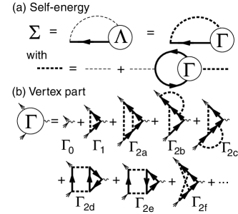
FIG. 1.: (a) Self-energy in diagrammatic representation. Thick solid and thin dashed lines indicate, respectively, the electron Green’s function and the bare phonon propagator. (b) Expansion series for the vertex $\Gamma$ up to second order in $\alpha$.

There is, however, an important difference in the vertex correction. In contrast to the Holstein system, the corrections represented by the diagrams $\Gamma_{1},\Gamma_{2a},\cdots,\Gamma_{2e}$ is seen to vanish in the JT system by merely considering the pseudospin assignment together with the direction of phonon propagators, because Eq. (4) dictates that the JT-phonon exchange interaction works only in the pseudospin exchange process between electrons with opposite pseudospins. Physically both electrons and phonons in the JT system are associated with a notion of clockwise- or counterclockwise-“rotation” around each JT center and electrons interact with phonons only when the total rotation is conserved. In this sense, the vanishment of these vertex corrections is due to the local-rotation conservation law. This law allows only processes such as the one represented by $\Gamma_{2f}$ for $\Gamma$. Similarly, all the third-order vertex corrections vanish. Ineffectiveness of the vertex correction widens the applicable range in $\alpha$ of the Migdal’s approximation in the JT system and it leads us to the smaller polaron mass enhancement factor $m^{*}/m$ than that in the Holstein model in which the correction $\Gamma_{1}$ is known to enhances $m^{*}/m$ as $\alpha$ increases.

The above perturbative approach is not useful in discussing a small polaron or polaron localization in a site. According to the studies on the Holstein model, [13] an ED calculation in a two-site system provides qualitatively correct and quantitatively fair results for the small polaron in the strong-coupling region ($\alpha\!>\!1$), irrespective of the value of $\tilde{t}$. Thus we shall make a similar analysis of a single electron in the JT model with $N=2$ in which the eigenvalues of the conserved quantity $L$ are half-integers and each energy level is doubly degenerate.

Let us consider the antiadiabatic region ($\tilde{t}\!\ll\!1$) first. At $\alpha\!\gg\!1$, both the ground and first-excited states belong to the sector of $|L|\!=\!1/2$. Using $\Psi^{(0)}_{j}$ in Eq. (6), their wavefunctions $\Psi_{\pm}$ are written as $\Psi_{\pm}\!\approx\!(\Psi^{(0)}_{1}\pm\Psi^{(0)}_{2})/\sqrt{2}$ for $L\!=\!1/2$ with the corresponding energies $E_{\pm}\!=\!E_{0}\pm t/[I_{0}(\alpha)\!+\!I_{1}(\alpha)]$. The energy difference, $E_{+}-E_{-}$, can be used to estimate the polaron bandwidth in a crystal and thus its ratio with the bare value, $2t$, determines the polaron effective mass through the relation

$${m\over m^{*}}={E_{+}-E_{-}\over 2t}={1\over I_{0}(\alpha)\!+\!I_{1}(\alpha)}\approx\sqrt{{\pi\alpha\over 2}}\,e^{-\alpha}.$$ (16)

This result should be compared with $e^{-2\alpha}$ the Holstein’s famous result [9] for the system defined in Eq. (15).

We resort to ED calculations to obtain $m/m^{*}$ through the numerical evaluation of $E_{\pm}$ for arbitrary $\alpha$. The conservation of $L$ helps reduce the number of expansion bases for phonons considerably. We plot the calculated $m/m^{*}$ for both JT and Holstein models in Fig. 2 in which $\tilde{t}$ is taken as $0.2$, although the result itself does not depend on $\tilde{t}$ provided that it is much smaller than unity. (The result for the Holstein model hardly changes from the analytic result $e^{-2\alpha}$ in the whole region of $\alpha$.) For small $\alpha$, both models give essentially the same $m/m^{*}$ as implied by the previous weak-coupling analysis. For large $\alpha$, however, there is a difference in $m^{*}/m$ which is more than orders of magnitude for $\alpha\!>\!1$, indicating that the JT polaron is quite mobile compared to the Holstein polaron.

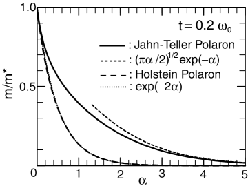
FIG. 2.: Polaron mass reduction factor $m/m^{*}$ for the JT (the solid curve) and the Holstein (the dashed curve) models with each analytic expression in the strong-coupling region.

Next we make a semiclassical argument on the adiabatic region ($\tilde{t}\!\gg\!1$) by considering the adiabatic potential $U_{\rm ad}$ for given phonon variables, $\{q_{1}\theta_{1};q_{2}\theta_{2}\}$. Since it was calculated previously in connection with the Berry phase,[21] we just give the result here as

$$U_{\rm ad}\! = \!{\omega_{0}^{2}\over 2}q^{2}\!-\!\Bigl{\{}t^{2}\!+\!\alpha{\omega_{0}}^{3}q^{2}\!+\!\bigl{\{}2\alpha{\omega_{0}}^{3}t^{2}[q^{2}\!+\!2q_{1}q_{2}$$ (18)

$$\times\cos(\theta_{1}\!-\!\theta_{2})]\!+\!\alpha^{2}{\omega_{0}}^{4}({q_{1}}^{2}\!-\!{q_{2}}^{2})^{2}\bigr{\}}^{1/2}\Bigr{\}}^{1/2},$$

with $q^{2}\!\equiv\!{q_{1}}^{2}\!+\!{q_{2}}^{2}$. This potential has rather simple features; if the adiabaticity parameter $\lambda\!\equiv\!\alpha/\tilde{t}\!=\!E_{\rm JT}/t$ is less than unity, $U_{\rm ad}$ has only one minimum in $\{q_{1}\theta_{1};q_{2}\theta_{2}\}$-coordinate space, implying no symptom for a small polaron. On the other hand, it is a double-well potential for $\lambda\!>\!1$ with the energy barrier $\Delta\!=\!(\alpha\omega_{0}/2)(1\!-\!\lambda^{-1})^{2}$. If the largest zero-point energy of phonons $\Delta_{\rm zero}$ (which is $\omega_{0}/2$ in this case) is smaller than $\Delta$, localization leading to a small polaron occurs. Thus the condition $\Delta\!\gtrsim\!\Delta_{\rm zero}$ provides the criterion to obtain a small polaron as

$$\tilde{t}\lesssim\alpha-\sqrt{\alpha},\quad{\rm with}\ \alpha>1.$$ (19)

A similar argument has been done for the Holstein model described in Eq. (15) for which a double-well potential appears only when $\lambda\!>\!1/2$ with $\Delta\!=\!\alpha\omega_{0}(1\!-\!1/2\lambda)^{2}$ and $\Delta_{\rm zero}\!=\!(\omega_{0}/2)\sqrt{1\!-\!1/4\lambda^{2}}$ [13], leading to the criterion

$$\alpha\Bigl{(}1-{1\over 2\lambda}\Bigr{)}^{2}\gtrsim{1\over 2}\sqrt{1-{1\over 4\lambda^{2}}}\,.$$ (20)

This condition cannot be reduced to such a simple form as that in (19), but clearly it is much less restrictive than (19) for the small-polaron formation.

Finally we make a more quantitative argument on the large-to-small polaron crossover based on the exact ground-state wavefunction $\Psi_{0}$ obtained by the ED calculation. We evaluate two quantitites, “the transfer amplitude per bond” $T\!\equiv\!\langle\Psi_{0}|\sum_{\sigma}(c^{+}_{1\sigma}c_{2\sigma}\!+\!c^{+}_{2\sigma}c_{1\sigma})|\Psi_{0}\rangle/N_{\rm bond}$ with the number of the bond $N_{\rm bond}\!=\!1$ and “the interaction amplitude per site” $I\!\equiv\!\langle\Psi_{0}|\sum_{j}\bigl{[}(a^{+}_{j}\!-\!b_{j})c^{+}_{j\uparrow}c_{j\downarrow}\!+\!(a_{j}\!-\!b^{+}_{j})c^{+}_{j\downarrow}c_{j\uparrow}\bigr{]}|\Psi_{0}\rangle/N$ with $N\!=\!2$. Then we measure “itineracy” by the ratio $|T/I|$, because the ratio must be large for an itinerant polaron.

Contour plots for $|T/I|$ in $(\tilde{t},\alpha)$-plane are given in Fig. 3. The result for the Holstein polaron indicates that the semiclassical criterion for the small-polaron formation corresponds to the condition $|T/I|\!\approx\!0.5$. More or less the same result is obtained for the JT polaron for which Eq. (19) is well represented by the condition $|T/I|\!\approx\!0.6$. In either way, we can conclude that the large-to-small polaron crossover occurs at around $|T/I|\!\approx\!0.5-0.6$ and that a small polaron is much harder to realize in the JT system than the Holstein one.

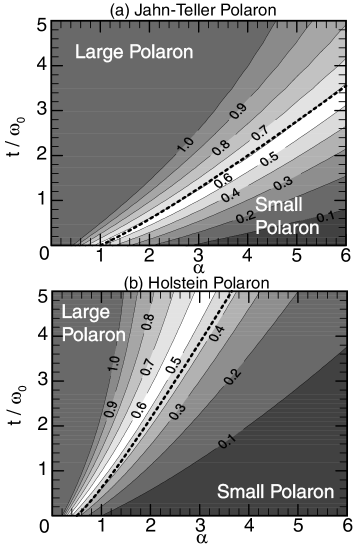
FIG. 3.: Contour plot for $|T/I|$ for (a) JT and (b) Holstein polarons. (Only the curves in the range $0.1-1.0$ are shown to avoid too many curves.) The thick dotted curves correspond to the semiclassical criteria to divide large and small polarons, Eqs. (19) and (20).

Three comments are in order: (1) In the manganese oxides, the parameters are estimated as $t\!\approx\!0.2$eV, $\omega_{0}\!\approx\!0.08$eV, and $E_{\rm JT}\!\approx\!0.2-0.4$eV, leading to $\tilde{t}\!\approx\!2.5$ and $\alpha\!\approx\!2.5-5$, which covers the crossover region according to Fig. 3(a). This is convenient to explain the observed CMR behavior. (2) The very large $m^{*}$ in the Holstein model is unfavorable for the bipolaron scenario for high-$T_{c}$ superconductivity. [22] In this respect, a smaller $m^{*}$ was suggested for the Fröhlich polaron. [23] The same may be claimed for the JT polaron. (3) The electron-phonon coupling constant in $H_{\rm H}$ [Eq. (15)] is so determined as to give the same polaron effect as the JT case in the weak-coupling region for the proper comparison of vertex corrections. In this choice, the ground-state energy for $H_{\rm H}$ at $t=0$ is given as $(-2\alpha\!+\!1/2)\omega_{0}$ which is about $-2E_{\rm JT}$ at $\alpha\!\gg\!1$. Thus, if we make an alternative choice of the coupling constant as to give the same polaron stabilization energy in the strong-coupling limit, the difference in $m^{*}$ between the JT and Holstein models looks to be much reduced, but even in this choice, the JT polaron has smaller $m^{*}$ at least by the factor of $1/\sqrt{\alpha}$.

In conclusion, we have compared the $E\otimes e$ JT polaron with the Holstein one by using various theoretical techniques. Features of these polarons are exactly the same in the weak-coupling region, but they are different quantitatively in other regions due to the symmetry of pseudospin rotation; the JT polaron is more mobile than the Holstein one.

The author is supported by the Grant-in-Aid for Scientific Research (C) from the Ministry of Education, Science, Sports, and Culture of Japan.

REFERENCES

• [1] A. J. Millis et al., Phys. Rev. Lett. 74, 5144 (1995).
• [2] G.-M. Zhao et al., Nature 381, 676 (1996); A.Shengelaya et al., Phys. Rev. Lett. 77, 5296 (1996).
• [3] S. J. L. Billinge et al., Phys. Rev. Lett. 77, 715 (1996).
• [4] For recent developments, see the review article: A. Mareo et al., Science 283, 2034 (1999).
• [5] H. RΓΆder et al., Phys. Rev. Lett. 76, 1356 (1996); J. Zang et al., Phys. Rev. B 53, R8840 (1996).
• [6] A. J. Millis et al., Phys. Rev. Lett. 77, 175 (1996); Phys. Rev. B 54, 5389, 5405 (1996).
• [7] J. D. Lee and B. I. Min, Phys. Rev. B 55, 12454 (1997).
• [8] H. FrΓΆhlich, Adv. Phys. 3, 325 (1954).
• [9] T. Holstein, Ann. Phys. (N.Y.) 8, 325, 343 (1959).
• [10] K.-H. HΓΆck et al., Helv. Phys. Acta 56, 237 (1983).
• [11] M. Fabrizio and E. Tosatti, Phys. Rev. B 55, 13465 (1997).
• [12] P. Benedetti and R. Zeyher, Phys. Rev. B 59, 9923 (1999).
• [13] A. S. Alexandrov and N. F. Mott, Polarons and Bipolarons, (World Scientific, Singapore, 1995); M. Capone et al., Phys. Rev. B 56, 4484 (1997); K. Yonemitsu et al., Phys. Rev. B 59, 1444 (1999).
• [14] G. Whitefield and R. Puff, Phys. Rev. 139, A338 (1965).
• [15] I. B. Bersuker and V. Z. Polinger, Vibronic Interactions in Molecules and Crystals, (Springer, Berlin, 1989).
• [16] We suppress spin indices for the JT polaron in order to avoid confusion between β€œreal” and β€œpseudo” spins.
• [17] The reduced mass of ions for the vibrational modes is normalized to unity.
• [18] For $L_{\bf j}\!=\!-1/2$, the operator $\sqrt{2/\alpha}\ b_{\rm j}c^{+}_{{\bf j}\uparrow}\!+\!c^{+}_{{\bf j}\downarrow}$ in Eq.Β (6) should be replaced by $c^{+}_{{\bf j}\uparrow}\!-\!\sqrt{2/\alpha}\ a_{\rm j}c^{+}_{{\bf j}\downarrow}$.
• [19] We take such units as $k_{\rm B}\!=\!\hbar\!=\!1$.
• [20] A. B. Migdal, Sov. Phys. JETP 7, 996 (1958).
• [21] Y. Takada et al., to appear in Int. J. Mod. Phys. B (cond-mat/9906128).
• [22] B. K. Chakraverty et al., Phys. Rev. Lett. 81, 433 (1998).
• [23] A. S. Alexandrov and P. E. Kornilovitch, Phys. Rev. Lett. 82, 807 (1999).