Monte Carlo Study of the Anisotropic Heisenberg
Antiferromagnet on the Triangular Lattice

Abstract

We report a Monte Carlo study of the classical antiferromagnetic Heisenberg model with easy axis exchange anisotropy on the triangular lattice. Both the free energy cost for long wavelength spin waves as well as for the formation of free vortices are obtained from the spin stiffness and vorticity modulus respectively. Evidence for two distinct Kosterlitz–Thouless types of defect-mediated phase transitions at finite temperatures is presented.

PACS numbers: 75.10.Hk, 75.40.Mg

I INTRODUCTION

The nature of phase transitions in frustrated systems are generally found to be quite different from those in conventional magnets.[1] Frustration often leads to non-trivial ground state degeneracies as in the case of the antiferromagnetic spin 1/2 Ising model on the triangular lattice. [2, 3] The classical Heisenberg model on the two dimensional triangular lattice with antiferromagnetic nearest neighbour coupling and easy axis exchange anisotropy is another example where frustration leads to a novel ground state degeneracy. Miyashita and Kawamura[4](MK) have investigated both the ground state and the nature of harmonic excitations at low temperatures in this model. At zero temperature the spins lie in a plane which contains the easy $z$-axis. In addition to the $S_{1}$ degeneracy related to the rotation of this plane about the $z$-axis, there is also a non-trivial $S_{1}$ degeneracy of the ground state related to rotations of the spins within the plane. The planar spin configuration distorts as it is rotated about an axis normal to the plane but the energy remains constant. This degeneracy is not broken by the harmonic excitations. Using Monte Carlo methods, MK measured the specific heat as well as various susceptibilities and suggested that the system undergoes two successive phase transitions as the temperature is lowered. The two transitions indicated the onset of power law correlations of the spin-spin correlation functions parallel and perpendicular to the easy axis. More recently, Sheng and Henley[5] have examined both the effects of finite temperature and quantum fluctuations on this non-trivial degeneracy. They predicted that the continuous degeneracy at finite temperatures $T$ is reduced to a discrete six-fold degeneracy and that an additional phase transition from a floating phase to a locked phase occurs at a temperature in between the upper and lower transitions for large values of the easy axis anisotropy.

In the present work, we use a direct method to study the free energy cost of both spin wave and vortex formation in this system at low temperatures. We define a spin stiffness and a vorticity modulus in terms of an equilibrium correlation function which can be evaluated using standard Monte Carlo methods. Our results indicate that there are only two transitions and that both correspond to vortex unbinding transitions accompanied by power law decay of spin correlations.

II The Model

The Hamiltonian of the system is given by

$$H=+\sum_{i<j}[{J^{x}S_{i}^{x}S_{j}^{x}+J^{y}S_{i}^{y}S_{j}^{y}+J^{z}S_{i}^{z}S_{j}^{z}}]$$ (1)

where ${S^{\alpha}_{i},\alpha=x,y,z}$ represents a classical 3-component spin of unit magnitude located at each site $i$ of a triangular lattice and the exchange interactions $J^{x}=J^{y}=J,J^{z}=AJ$ are restricted to nearest neighbour pairs of sites. We shall consider the case where the parameter range A $\geq$ 1 represents an easy axis anisotropy. The limit $A\rightarrow 1$ corresponds to the isotropic Heisenberg model[6] whereas the limit $A\rightarrow\infty$ corresponds to an infinite spin Ising model.[7] Southern and Xu[8] have previously studied the Heisenberg limit and found direct evidence for a vortex unbinding transition at finite temperature even though the spin stiffness vanishes on large length scales. This latter fact indicates that the spin correlations decay exponentially at all finite temperatures $T$. This behaviour is quite different from that which occurs in the corresponding two-component $xy$ model[9] where power law decay of the correlations appear at low temperatures.

The triangular lattice can be decomposed into three sublattices $A,B$ and $C$ as shown in figure 1 with the three spins on each triangle labelled as ${\bf S}_{A},{\bf S}_{B}$ and ${\bf S}_{C}$. A chirality vector[10] for each upward pointing triangle is defined as follows

$${\bf K_{\Delta}}=\frac{2}{3\sqrt{3}}({\bf S}_{A}\times{\bf S}_{B}+{\bf S}_{B}\times{\bf S}_{C}+{\bf S}_{C}\times{\bf S}_{A})$$ (2)

FIG. 1.: The decomposition of the triangular lattice into three sublattices $A,B$ and $C$. The sublattice labels on all black triangles are the same and represent only one of the six possible choices.

In the present case of the easy axis antiferromagnet, the low temperature spin configuration on each triangle has the spins lying in a plane which includes the $z$-axis and which is perpendicular to the chirality vector. We introduce a local spin space coordinate system for each upward pointing triangle using the three unit vectors $\hat{\bf K}_{\Delta},\hat{\bf z}$ and $\hat{\bf{\perp}}_{\Delta}=\hat{\bf z}\times\hat{\bf K}_{\Delta}$. Hence the vectors $\hat{\bf z}$ and $\hat{\bf\perp}_{\Delta}$ lie in the spin plane and $\hat{\bf K}_{\Delta}$ is the local normal to the plane. The $\hat{\bf z}$ is a global axis for all triangles whereas the $\hat{\bf K}_{\Delta}$ are only all aligned at $T=0$. As $T$ increases, the local normal directions fluctuate and the spin plane develops curvature. Hence local coordinates are needed to properly define the response properties of the system.

Information about the rigidity of the system against fluctuations can be obtained from the spin wave stiffness coefficient. The spin stiffness (helicity) tensor is given by the second derivative of the free energy[11, 12] with respect to the twist angle about a particular direction in spin space. We apply a twist about each of the local axes defined above and the corresponding average stiffness is given by

$$\rho_{\alpha} = -\frac{1}{N}\sum_{i<j}(\hat{\bf e}_{ij}\cdot\hat{\bf u})^{2}\langle J^{\beta}S_{i}^{\beta}S_{j}^{\beta}+J^{\gamma}S_{i}^{\gamma}S_{j}^{\gamma}\rangle$$ (4)

$$-\frac{1}{NT}\langle(\sum_{i<j}(\hat{\bf e}_{ij}\cdot\hat{\bf u})[\frac{J^{\beta}+J^{\gamma}}{2}][S_{i}^{\beta}S_{j}^{\gamma}-S_{i}^{\gamma}S_{j}^{\beta}])^{2}\rangle$$

where the superscipts take the values $\alpha=\perp_{\Delta},z,K_{\Delta}$ and $\alpha,\beta,\gamma$ are to be taken in cyclic order. $S_{i}^{\alpha}$ denotes the component of the spin at site $i$ in the average direction of the corresponding local unit vectors of the upward pointing triangles to which the spin belongs, $\hat{\bf e}_{ij}$ are unit vectors along neighbouring bonds and $\hat{\bf u}$ is the direction of the twist in the lattice.

We employ compact clusters, as shown in figure 2, containing $N$ spins with periodic boundary conditions applied that are consistent with the sublattice structure. The number of spins is related to the linear size $L$ of the cluster as $N=3L^{2}$.

FIG. 2.: Compact clusters of linear size $L$ containing $N=3L^{2}$ spins used in the Monte Carlo calculations are indicated by the solid lines. In each case periodic boundary conditions are used which are compatible with the three sublattice structure.

We have used a single spin-flip heat bath algorithm[13] to update the spin directions at each Monte Carlo step and all thermal averages are replaced by time averages. For the largest value of the system size $L=60$ studied we discard the first $1.5\times 10^{4}$ Monte Carlo steps and perform averages over the next $5\times 10^{5}$ steps.

The values of the stiffnesses at zero temperature can be evaluated using the exact classical ground state correlation functions. We find these values to be

$$\rho_{z}/{J} = \frac{2A+1}{2(1+A)^{2}}$$ (5)

$$\rho_{\perp}/{J} = A^{2}\frac{A+2}{2(1+A)^{2}}$$ (6)

$$\rho_{K} = \rho_{z}+\rho_{\perp}$$ (7)

These three stiffnesses satisfy a perpendicular axis theorem which is consistent with the ground state being a planar spin arrangement. In the Heisenberg limit we have $\rho_{z}=\rho_{\perp}$ but for large values of $A$ they have different energy scales, ${\rho_{z}}/{J}\sim\frac{1}{A}$ whereas ${\rho_{\perp}}/{J}\sim\frac{A}{2}$. These limiting values can also be obtained from the harmonic excitation spectrum.[5]

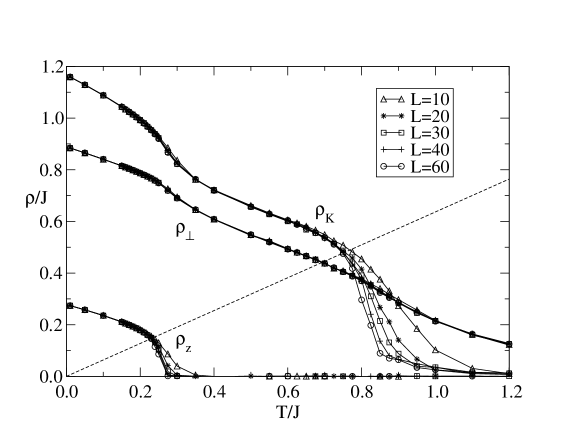
FIG. 3.: The three stiffnesses $\rho_{z},\rho_{\perp}$ and $\rho_{K}$ in units of $J$ as a function of $T/J$ for system sizes $L=10,20,30,40,60$ when $A=2$. The dashed curve represents the line $\rho=(2/\pi)T$.

Figure 3 shows the results obtained for the three stiffnesses as a function of $T/J$ for various system sizes $L$ with $A=2$. As the temperature increases towards $T_{c_{1}}=(0.231\pm 0.005)J$, the stiffness corresponding to the smaller energy scale, $\rho_{z}$, decreases abruptly and a strong dependence on system size $L$ is evident indicating that above this temperature the system has no rigidity against twists of the spins about the easy axis. MK suggested that this transition corresponds to the unbinding of vortices associated with the chirality vector which lies primarily in the $xy$ plane. We will provide further support for this interpretation in section IV.

The remaining two stiffnesses do not vanish at $T_{c_{1}}$ but do exhibit a rapid decrease followed by a more steady decrease until a higher temperature $T_{c_{2}}=(0.75\pm 0.03)J$. At this higher temperature, the strong dependence of the stiffness $\rho_{K}$ on system size $L$ indicates that the system loses rigidity against rotations about the local chirality axes. The Kosterlitz-Thouless(KT) theory[14, 15, 16] for the $xy$ model in two dimensions predicts a universal value for the ratio ${\rho_{c}}/{T_{c}}$ equal to $2/\pi$. The dashed line in figure 3 corresponds to $\rho/T={2}/{\pi}$ and intersects the stiffnesses at temperatures where finite size effects first appear. The stiffnesses $\rho_{z}$ and $\rho_{K}$ indicate two temperatures where rigidity of the system about the $z$-axis is first lost followed by a loss of rigidity about the local chirality axis with an apparent universal value for the ratio $\rho_{c}/T_{c}$ in each case. The third stiffness $\rho_{\perp}$ has a change in curvature at the two transitions but remains finite to high temperatures. Similar behaviour is found for other values of $A$ as well.

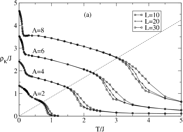
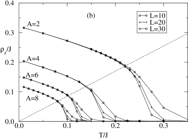
FIG. 4.: The spin stiffnesses (a) $\rho_{K}$ and (b) $\rho_{z}$ in units of $J$ as a function of $T/J$ for system sizes $L=10,20,30$ with $A=2,4,6,8$. The dashed curve in both cases represents the line $\rho=(2/\pi)T$.

Figures 4(a) and 4(b) show our results for $\rho_{K}$ and $\rho_{z}$ respectively for the values $A=2,4,6,8$. The dashed line plotted in both figures corresponds to $\rho/T={2}/{\pi}$ and in each case this line intersects the stiffnesses at the temperatures where finite size effects first become significant. These results indicate that the ratio ${\rho_{c}}/{T_{c}}$ appears to have the universal value ${2}/{\pi}$ for both stiffnesses for all values of $A>1$. We have used this criterion to estimate the values of $T_{c_{1}}$ and $T_{c_{2}}$.

In the same way that the spin stiffness is a measure of the response of the spin system to a twist over the length of the lattice, a vorticity[8] can be defined as the response of the spin system to an imposed twist about a given axis $\alpha$ in spin space along a closed path which encloses a vortex core. This is essentially the response of the system to an isolated vortex and can be calculated as the second derivative of the free energy with respect to the strength of the vortex, or winding number $m$, evaluated at $m=0$. We obtain the following expression

$$V_{\alpha} = -\frac{\sqrt{3}}{4\pi}\sum_{i<j}(\frac{\hat{\bf e}_{ij}\cdot\hat{\bf\phi_{i}}}{r_{i}})^{2}\langle J^{\beta}S_{i}^{\beta}S_{j}^{\beta}+J^{\gamma}S_{i}^{\gamma}S_{j}^{\gamma}\rangle$$ (9)

$$-\frac{\sqrt{3}}{4\pi T}\langle(\sum_{i<j}(\frac{\hat{\bf e}_{ij}\cdot\hat{\bf\phi_{i}}}{r_{i}})[\frac{J^{\beta}+J^{\gamma}}{2}][S_{i}^{\beta}S_{j}^{\gamma}-S_{i}^{\gamma}S_{j}^{\beta}])^{2}\rangle$$

where $r_{i}$ is the distance of site $i$ from the vortex core and $\hat{\bf\phi_{i}}$ is tangent to the circular path in the lattice passing through the site $i$ and enclosing the vortex. Here $\alpha,\beta,\gamma$ are defined in the same way as for the stiffnesses and indicate the axis of rotation of the vortex.

The $V_{\alpha}$ contain both a core contribution and a part which is proportional to ln$L$. By comparing systems of different lattice sizes $L_{1}$ and $L_{2}$ we can extract the vorticity modulus $v_{\alpha}$ defined as follows

$$V_{\alpha}=C_{\alpha}+v_{\alpha}\ln L$$ (10)

using

$$v_{\alpha} = \frac{V_{\alpha}(L_{2})-V_{\alpha}(L_{1})}{\ln(L_{2}/L_{1})}$$ (11)

where the $v_{\alpha}$ are normalized so that they have the same zero temperature values as the corresponding stiffnesses. Our approach does not require any change in boundary conditions and is applied directly to the antiferromagnetic model.

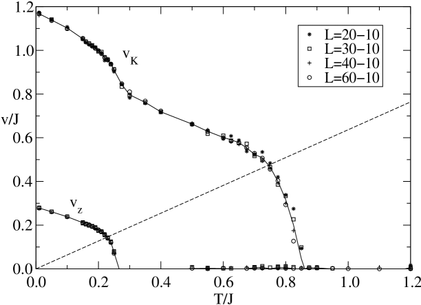
FIG. 5.: The vorticity moduli $v_{K}$ and $v_{z}$ in units of $J$ as a function of $T/J$ obtained using various pairs of system sizes when $A=2$. The solid curves represent the average of all pairs for each modulus. The dashed curve represents the line $v=(2/\pi)T$.

Figure 5 shows our results for the vorticity moduli obtained by comparing systems of different sizes when $A=2$. The behaviour of the moduli as a function of increasing temperature is identical to the spin stiffnesses shown in figure 3. The vorticity modulus $v_{\perp}$ is only weakly sensitive to the two transitions and is not plotted. The vanishing of the vorticity moduli $v_{z}$ and $v_{K}$ at $T_{c_{1}}$ and $T_{c_{2}}$ respectively indicates that free vortices appear at these two transition temperatures. The results are also consistent with a universal value $v_{c}/T_{c}=2/\pi$. Similar behaviour is found for the values $A=2,4,6,8$.

The results presented so far do not indicate directly that power law decay of correlations are present below these two transition temperatures. In the next section we present results for the spin-spin structure factor which are also consistent with KT transitions.

III Structure Factor

We have also studied the spin-spin structure factor for various system sizes $L$

$$S^{\alpha\alpha}({\bf q})=\frac{1}{N}\sum_{i,j}<S^{\alpha}_{i}S^{\alpha}_{j}>e^{i{\bf q}.({\bf r}_{i}-{\bf r}_{j})}$$ (12)

where $\alpha=x,y,z$ . In particular, we have studied $S^{\perp}=S^{xx}+S^{yy}$ and $S^{zz}$ as a function of both ${\bf q}$ and $T$. In both cases the Fourier component ${\bf Q}=(4\pi/3,0)$ exhibits a divergence at and below the two transition temperatures $T_{c_{1}}$ and $T_{c_{2}}$ respectively. Other values of ${\bf q}$ only exhibit a maximum. This Fourier component corresponds to the three-sublattice structure associated with the triangles. If we assume power law decay of the spin-spin correlation functions, then the structure factors should depend on the system size $L$ as follows

$$S^{zz}({\bf Q}) \sim L^{2-\eta_{z}}$$ (13)

$$S^{\perp}({\bf Q}) \sim L^{2-\eta_{\perp}}$$ (14)

where $\eta_{z}$ and $\eta_{\perp}$ are the corresponding correlation length exponents.

FIG. 6.: The correlation function exponents $2-\eta_{\perp}$ and $2-\eta_{z}$ as a function of $T/J$ obtained by comparing various system sizes with $A=2$. The dashed line corresponds to $\eta=1/4$.

Figure 6 shows the values of $2-\eta_{z}$ and $2-\eta_{\perp}$ as a function of $T/J$ obtained by comparing systems of different sizes with $A=2$. The dashed line indicates the value $\eta=1/4$ predicted by the KT theory and intersects both exponents at temperatures where a strong dependence on system size first appears. Similar results were obtained for other values of $A$. The universal value of $\eta_{z}=\eta_{\perp}=1/4$ is consistent with the universal value of $\rho_{c}/T_{c}=2/\pi$ and $v_{c}/T_{c}=2/\pi$ obtained in section II.

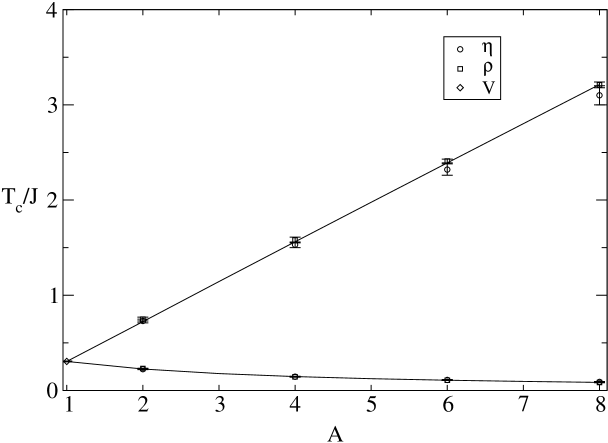
FIG. 7.: The transition temperatures $T_{c_{1}}/J$ (lower) and $T_{c_{2}}/J$ (upper) as a function of $A$ determined using the universal value of the stiffness $\rho$ and the universal value of $\eta$ are shown by the squares and circles respectively. The value at the Heisenberg point ($A=1$) is indicated by the diamond and was obtained from previous vorticity results. The solid curves are obtained by assuming that these two temperatures are proportional to the $T=0$ values of $\rho_{z}$ and $\rho_{\perp}$ respectively.

We have used these two criteria to obtain the temperatures $T_{c}{{}_{1}}$ and $T_{c}{{}_{2}}$ as a function of $A$ as shown in figure 7. The values obtained from the stiffnesses and the structure factors agree with each other fairly well. The error bars in $T_{c}$ reflect contributions from the statistical uncertainty of the Monte Carlo measurements, as well as estimated systematic contributions due to finite size effects. If we make the simple assumption that the dependence of $T_{c_{1}}$ and $T_{c_{2}}$ on $A$ is the same as the zero temperature values of $\rho_{z}$ and $\rho_{\perp}$ respectively, then we have

$$T_{c_{1}} = T_{c}\ \frac{4(2A+1)}{3(1+A)^{2}}$$ (15)

$$T_{c_{2}} = T_{c}\ \frac{4A^{2}(A+2)}{3(1+A)^{2}}$$ (16)

where the values of $T_{c_{1}}$ and $T_{c_{2}}$ in the isotropic limit $A=1$ are both equal to $T_{c}=(.305\pm.005)J$.[8] These expressions are plotted as the solid curves in figure 7 and the agreement with the data points is remarkable.

The limit $A\rightarrow\infty$ of the present model is equivalent to the $S\rightarrow\infty$ limit of the antiferromagnetic spin $S$ Ising model on the same lattice with coupling $AJ$. The solid curve for $T_{c_{2}}$ approaches the value $T_{c}{{}_{2}}/AJ\sim.407\pm.007$ in this limit. This value is also in excellent agreement with that obtained by Nagai et al.[17] for the $S=\infty$ Ising model. In the next section we give a more detailed microscopic description of these phases.

IV Microscopic Properties

The three spins ${\bf S}_{A},{\bf S}_{B}$ and ${\bf S}_{C}$ on each triangle can be expressed in terms of the following three vectors

$${\bf M}_{0} = {\bf S}_{A}+{\bf S}_{B}+{\bf S}_{C}$$ (17)

$${\bf M}_{R} = {\bf S}_{A}-\frac{1}{2}{\bf S}_{B}-\frac{1}{2}{\bf S}_{C}$$ (18)

$${\bf M}_{I} = \frac{\sqrt{3}}{2}({\bf S}_{B}-{\bf S}_{C})$$ (19)

The vectors ${\bf M}_{R}$ and ${\bf M}_{I}$ are the real and imaginary parts of the complex Fourier component ${\bf M}_{\bf Q}={\bf M}_{R}+i{\bf M}_{I}$ where ${\bf Q}=(4\pi/3,0)$. In addition, the chirality for each triangle can be written as ${\bf K}=\frac{4}{9}{\bf M}_{R}\times{\bf M}_{I}$.

In the ground state the three spins lie in a plane which includes the $z$-axis. We denote the angle that each sublattice spin makes with the $z$-axis by $\theta_{\alpha}$, and define

$$\psi=(\theta_{A}+\theta_{B}+\theta_{C})/3$$ (20)

where $0\leq\psi\leq 2\pi$. We measure $\psi$ relative to the $z$-axis in the counter-clockwise direction. As discussed by Sheng and Henley[5], the nontrivial degeneracy of the ground state can be parameterized in terms of the angle $\psi$. It has been previously pointed out that both the energy and the magnitude of ${\bf M}_{0}$ are constant in the ground state manifold[5, 18]. However, it is easy to show that the modulus of the complex vector ${\bf M}_{\bf Q}$ is also constant. In the Appendix we give some exact results for the components of these vectors in the ground state. The $\perp,z$ components of these two vectors depend on $\psi$ in quite different ways. The components of ${\bf M}_{0}$ have periodicity $2\pi/3$ whereas the vectors ${\bf M}_{R}$ and ${\bf M}_{I}$ have period $2\pi$.

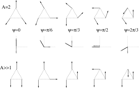
FIG. 8.: Ground state spin configurations for values of $\psi$ in the range $0\leq\psi\leq 2\pi/3$ for $A=2$ and $A\gg 1$. The horizontal and vertical axes are $\perp$ and $z$ repsectively. The corresponding directions of ${\psi}$ and ${\bf M}_{0}$ are independent of the value of $A$ and are indicated in the middle row by the solid and dashed arrows respectively.

Figure 8 shows ground state spin configurations of the sublattices in the $\perp,z$ plane for values of $\psi$ in the range $0\leq\psi\leq 2\pi/3$. The top row corresponds to $A=2$ and the bottom row to $A\rightarrow\infty$. Also shown are the corresponding directions of ${\psi}$ and ${{\bf M}}_{0}$ which are independent of the value of $A$. Rotations of the angle $\psi$ by $2\pi/3$ correspond to interchanges of the sublattice spin directions and to a complete rotation of ${\bf M}_{0}$ by $2\pi$. Hence vortex-like configurations of ${\bf M}_{0}$ simply correspond to switches of the sublattice magnetizations. For large values of the easy axis anisotropy, the spin configurations become more Ising-like. In the range $0\leq\psi\leq\pi/3$, sublattices $A$ and $B$ remain locked parallel to the easy axis while sublattice $C$ simply follows ${\bf M}_{0}$. In the range $\pi/3\leq\psi\leq 2\pi/3$, the roles are interchanged with sublattice $A$ following the direction of ${\bf M}_{0}$. These sublattice changes as a function of $\psi$ are similar to the domain transition regions described by Wannier[2] for the $S=1/2$ Ising model at $T=0$. In this latter case, the transition regions contribute to the macroscopic entropy of the system and to the power law decay of correlations with wavevector ${\bf Q}$. [3]

The moduli of the complex numbers $M^{z}_{\bf Q}=M^{z}_{R}+iM^{z}_{I}$ and $M^{\perp}_{\bf Q}=M^{\perp}_{R}+iM^{\perp}_{I}$ are not constant in the ground state but the combination

$$M^{z}_{\bf Q}+iM^{\perp}_{\bf Q}=\sqrt{\frac{(4A+2)(A+2)}{(1+A)^{2}}}e^{i\Psi}$$ (21)

has constant modulus and a phase angle $\Psi$ which has a leading term linear in $\psi$ but with an additional small 6-fold modulation. At low temperatures the chirality vector lies in the $xy$ plane and it can be described by the complex number

$$K_{x}+iK_{y}=\sqrt{K^{2}_{x}+K^{2}_{y}}e^{i\Theta}$$ (22)

where the modulus is not constant but exhibits only a weak $\cos(6\psi)$ variation in the ground state. These two phase angles $\Theta$ and $\Psi$ describe the complex order parameters associated with the transitions at $T_{c_{1}}$ and $T_{c_{2}}$ respectively.

Our Monte Carlo procedure permits us to take snapshots of the spin configurations at various temperatures. In order to separate the topological defects from the continuous deformations of the spin configurations, we first raise the temperature to some fixed value and allow the system to reach equilibrium. We then rapidly quench the system to low temperatures and allow the system to approach a nonequilibrium configuration. The topological defects are metastable at low temperatures and require a much longer time to disappear than the continuous deformations. In figures 9 and 10 we show snapshots of the spin configuration at very low temperatures obtained by heating the system above $T_{c_{1}}$ and $T_{c_{2}}$ respectively and then rapidly quenching. In both cases, (a) describes the spatial variation of the chirality angle $\Theta$ and (b) describes the angle $\psi$.

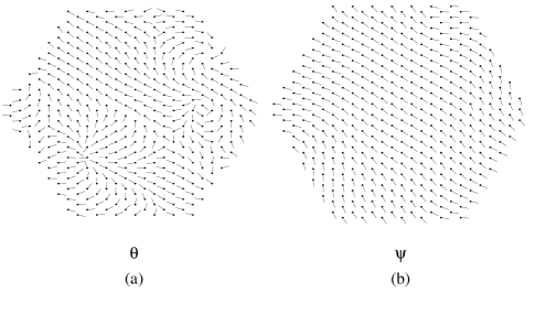
FIG. 9.: Snapshots of (a) the chirality angle $\Theta$ and (b) the angle $\psi$ at very low temperature following a quench from just above $T_{c_{1}}$ for $A=2$ and $L=20$. The dots indicate the positions of the black triangles shown in figure 1 and the lines indicate the local direction of either $\Theta$ or $\psi$.

Figure 9 shows snapshots of the spin configuration for a cluster of size $L=20$ with $A=2$ after quenching from a temperature of $T=0.5J$, just above $T_{c_{1}}$. Vortices associated with the angle $\Theta$ are clearly visible in (a) whereas only continuous distortions of the angle $\psi$ are visible in (b). These vortices in $\Theta$ only persist at low $T$ if the system is first heated to a $T>T_{c_{1}}$ and then quenched. They are metastable configurations at this lower temperature but become stable at $T_{c_{1}}$. Our results provide direct evidence for a vortex unbinding transition at $T_{c_{1}}$ involving the chirality vector.

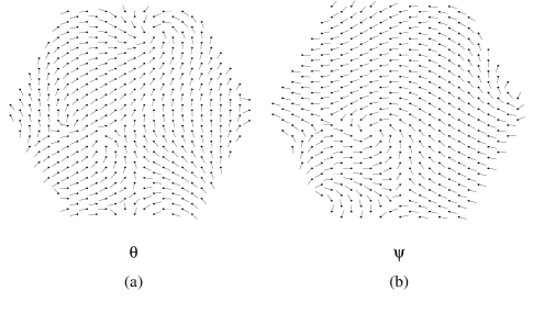
FIG. 10.: Snapshots of (a) the chirality angle $\Theta$ and (b) the angle $\psi$ at very low temperature following a quench from above $T_{c_{2}}$ for $A=2$ and $L=20$. The dots indicate the positions of the black triangles shown in figure 1 and the lines indicate the local direction of either $\Theta$ or $\psi$.

Figure 10 shows similar snapshots when the system is first heated to a temperature $T=3J$, well above $T_{c_{2}}$, and then rapidly quenched. Vortices in both $\Theta$ and $\psi$ are clearly visible in this case. The vortices in $\psi$ are only visible after quenching from above $T_{c_{2}}$. Hence the upper transition corresponds to a vortex unbinding transition associated with the sublattice ordering vector ${\bf M}_{\bf Q}$.

We have also studied how the sublattice magnetizations change as we update the spin configurations. In the temperature range $T<T_{c_{2}}$ there is a continuous sublattice switching that occurs. The time scale for the switching depends both on $T$ and system size $L$ increasing with $L$ and $1/T$. We have not been able to determine a scaling form for this time scale. Similar behaviour has been reported previously for other frustrated systems on the triangular lattice. The antiferromagnetic spin $1/2$ Ising model with both nearest and next-nearest neighbour interactions[19, 20] as well as the antiferromagnetic $S=\infty$ nearest neighbour model[7, 21, 22] exhibit this phenomena in the temperature range where a KT phase occurs. In our case, the switching is due to the wave-like variations in $\psi$ which can produce “vortex-like” variations in the local magnetization vector ${\bf M}_{0}$. In the range of $A$ that we have studied, we have not observed a transition from sublattice switching to a partially ordered phase where one of the sublattices is locked in the $+z$ direction, another in the $-z$ direction and the third perpendicular to the $z$-axis. Sheng and Henley[5] predicted that such a locking transition might occur at low enough temperature.

V Summary

We have presented strong evidence for the occurence of two distinct Kosterlitz-Thouless types of defect-mediated phase transitions in the Heisenberg antiferromagnet on the triangular lattice with easy axis anisotropy. A numerical approach was used to calculate the rigidity of the system against both spin wave deformations and the formation of free vortices at low temperatures for several values of the easy axis anisotropy. In each case a universal value of the stiffness or vorticity modulus, $\rho_{c}/T_{c}=v_{c}/T_{c}=2/\pi$, was found. In addition, the spin correlation length exponent has the universal value $\eta=1/4$. These are the same values that are predicted by the Kosterlitz-Thouless theory for defect unbinding transitions in two dimensions. The two phase angles identified in equations (13) and (14) in section IV describe the complex order parameters associated with the transitions at $T_{c_{2}}$ and $T_{c_{1}}$ respectively.

We find that the spin stiffnesses and the corresponding vorticity moduli behave identically for the easy axis case $A>1$. In contrast, at the isotropic Heisenberg limit, the spin stiffness vanishes at large length scales whereas the vorticity moduli are non-zero at low T and vanish abruptly at a finite temperature.[8] Our previous work on the $xy$ model [9] also indicated that the vorticity and stiffness behave identically. This corresponds to the $A\rightarrow-\infty$ limit where there are again two transitions but they are very close in temperature with the upper transition corresponding to an Ising-like transition and the lower to a Kosterlitz-Thouless transition. Recent work by Capriotti et. al. [23] has also found similar behaviour in the range $0<A<1$. Hence the Heisenberg point is a multicritical point where four phase transition lines meet. For $A>1$ there are two KT transition lines whereas as for $A<1$ there is an Ising and KT line.

VI Acknowledgements

This work was supported by the Natural Sciences and Engineering Research Council of Canada.

Miyashita and Kawamura[4] were the first to identify the nontrivial degeneracy of the ground state configuration. Other groups[5, 18] have studied the effects of quantum fluctuations on this degeneracy. One indicator of the degeneracy is that the magnetization vector ${\bf M}_{0}$ has a constant magnitude in the ground state independent of the value of $\psi$. In particular we find the following exact relations

$$M^{\perp}_{0} = -(\frac{A-1}{A+1})\sin(3\psi)$$ (23)

$$M^{z}_{0} = -(\frac{A-1}{A+1})\cos(3\psi)$$ (24)

$${\bf M}_{0}.{\bf M}_{0} = (\frac{A-1}{A+1})^{2}$$ (25)

where $\psi$ is measured counter-clockwise from the $z$-axis in the $\perp,z$ plane. A rotation of ${\bf M}_{0}$ by $2\pi$ corresponds to rotating $\psi$ by $2\pi/3$ which is simply a cyclic permutation of the sublattices on the triangle. Hence vortices in ${\bf M}_{0}$ can be associated with sublattice switching.

In addition to ${\bf M}_{0}$, the complex vector ${\bf M_{Q}}$ also has constant modulus,

$${\bf M}_{\bf Q}.{\bf M}_{\bf-Q} = {\bf M}_{R}.{\bf M}_{R}+{\bf M}_{I}.{\bf M}_{I}$$ (27)

$$= \frac{4A^{2}+10A+4}{(1+A)^{2}}$$ (28)

The moduli of the components of ${\bf M}_{\bf Q}$ as well, as the chirality, are not constant in the ground state but depend on $\psi$ as follows

$$|M_{Q}^{z}|^{2} = \frac{3A^{2}+6A}{(1+A)^{2}}+(\frac{A-1}{A+1})^{2}\cos^{2}(3\psi)$$ (29)

$$|M_{Q}^{\perp}|^{2} = \frac{6A+3}{(1+A)^{2}}+(\frac{A-1}{A+1})^{2}\sin^{2}(3\psi)$$ (30)

$$|{\bf K}|^{2} = \frac{4}{3\sqrt{3}}[\frac{\sqrt{2A+A^{2}}}{(A+1)^{2}}(2+A)\cos^{2}(3\psi)$$ (32)

$$\ \ \ \ \ \ +\frac{\sqrt{1+2A}}{(1+A)^{2}}(1+2A)\sin^{2}(3\psi)]$$

REFERENCES

- [1] H. Kawamura, J. Phys.: Condens. Matter 10, 4707 (1998).
- [2] G.H. Wannier, Phys. Rev. 79, 357 (1950).
- [3] J. Stephenson, J. Math. Phys. 5, 1009 (1964).
- [4] S. Miyashita and H. Kawamura, J. Phys. Soc. Japan 54, 3385 (1985).
- [5] Q. Sheng and C.L. Henley, J. Phys.: Condens. Matter 4, 2937 (1992).
- [6] H. Kawamura and S. Miyashita, J. Phys. Soc. Japan 53 ,4138 (1984).
- [7] T. Horiguchi, O. Nagai, S. Miyashita, Y. Miyatake and Y. Seo, J. Phys. Soc. Japan 61, 3114 (1992).
- [8] B.W. Southern and H-J. Xu, Phys. Rev. B52, R3836 (1995).
- [9] H-J. Xu and B.W. Southern, J. Phys. A: Math. Gen. 29, L133 (1996).
- [10] S. Miyashita and H. Shiba, J. Phys. Soc. Japan, 53, 1145 (1984).
- [11] B.W. Southern and A.P. Young, Phys. Rev. B48, 13170 (1993).
- [12] M. Caffarel, P. Azaria, B. Delamotte and D. Mouhanna, Europhys. Lett. 26, 493 (1994).
- [13] J.A. Olive, A.P. Young and D. Sherrington, Phys. Rev. B34, 6341 (1986).
- [14] J.M. Kosterlitz and D.J. Thouless, J. Phys. C: Solid State Phys., 6, 1181 (1973).
- [15] J.M. Kosterlitz, J. Phys. C: Solid State Phys., 7, 1046 (1974).
- [16] D.R. Nelson and J.M. Kosterlitz, Phys. Rev. Lett., 39, 1201 (1977).
- [17] O. Nagai, T. Horiguchi and S. Miyashita, in Magnetic Systems with Competing Interactions (Frustrated Spin Systems), ed. H.T. Diep (World Scientific, 1994), p. 220 .
- [18] B. Kleine, E. Műller-Hartmann, K. Frahm and P. Fazekas, Z. Phys. B87, 103 (1992).
- [19] S. Fujiki, K. Shutoh, Y. Abe and S. Katsura, J. Phys. Soc. Japan, 52, 1531 (1983).
- [20] H. Takayama, K. Matsumoto, H. Kawahara and K. Wada, J. Phys. Soc. Japan, 52, 2888 (1983).
- [21] O. Nagai, S. Miyashita and T. Horiguchi, Phys. Rev. B47, 202 (1993).
- [22] T. Horiguchi, O. Nagai, H.T. Diep and Y. Miyatake, Phys. Lett. A177, 93 (1993).
- [23] L. Capriotti, R. Vaia, A. Cuccoli and V. Tognetti, Phys. Rev. B58, 273 (1998).