Renormalization-Group Approach to the Vulcanization Transition

Abstract

The vulcanization transition—the crosslink-density-controlled equilibrium phase transition from the liquid to the amorphous solid state—is explored analytically from a renormalization group perspective. The analysis centers on a minimal model which has previously been shown to yield a rich and informative picture of vulcanized matter at the mean-field level, including a connection with mean-field percolation theory (i.e. random graph theory). This minimal model accounts for both the thermal motion of the constituents and the quenched random constraints imposed on their motion by the crosslinks, as well as particle-particle repulsion which suppresses density fluctuations and plays a pivotal role in determining the symmetry structure (and hence properties) of the model. A correlation function involving fluctuations of the amorphous solid order parameter, the behavior of which signals the vulcanization transition, is examined, its physical meaning is elucidated, and the associated susceptibility is constructed and analyzed. A Ginzburg criterion for the width (in crosslink density) of the critical region is derived and is found to be consistent with a prediction due to de Gennes. Inter alia, this criterion indicates that the upper critical dimension for the vulcanization transition is six. Certain universal critical exponents characterizing the vulcanization transition are computed, to lowest nontrivial order, within the framework of an expansion around the upper critical dimension. This expansion shows that the connection between vulcanization and percolation extends beyond mean-field theory, surviving the incorporation of fluctuations in the sense that pairs of physically analogous quantities (one percolation-related and one vulcanization-related) are found to be governed by identical critical exponents, at least to first order in the departure from the upper critical dimension (and presumably beyond). The relationship between the present approach to vulcanized matter and other approaches, such as those based on gelation/percolation ideas, is explored in the light of this connection. To conclude, some expectations for how the vulcanization transition is realized in two dimensions, developed with H. E. Castillo, are discussed.

I Introduction

Whilst a rather detailed description of the vulcanization transition has emerged over the past few years within the context of a mean-field approximation [1, 2, 3, 4], the picture of this transition beyond the mean-field level is less certain. The purpose of the present Paper is to provide a description of the vulcanization transition beyond the mean-field approximation via the application of renormalization group (RG) ideas to a model that incorporates both the quenched randomness (central to systems undergoing the vulcanization transition) and the thermal fluctuations of the constituents (whose change in character is the fundamental hallmark of the transition). Our aim is to shed some light on certain universal properties of the vulcanization transition within the framework of the well-controlled and systematically improvable approximation scheme that the RG provides, viz., an expansion about an upper critical dimension that we shall see takes the value six.

We remind the reader that the vulcanization transition is an equilibrium phase transition from a liquid state of matter to an amorphous solid state. (In addition to the technical reports cited above [1, 2, 3, 4], we refer the reader to some informal accounts of the physics of the vulcanization transition [5, 7, 8].)  The transition occurs when a sufficient density of permanent random constraints (e.g. chemical crosslinks)—the quenched randomness—are introduced to connect the constituents (e.g. macromolecules), whose locations are the thermally fluctuating variables. In the resulting amorphous solid state, the thermal motion of (at least a fraction of) the constituents of the liquid undergo a qualitative change: no longer wandering throughout the container, they are instead localized in space at random positions about which they execute thermal (i.e. Brownian) motion characterized by random r.m.s. displacements.

Our approach to the vulcanization transition is based on a minimal Landau-Wilson effective Hamiltonian that describes the energetics of various order-parameter-field configurations, the order parameter in question having been crafted to detect and diagnose amorphous solidification. This order parameter and effective Hamiltonian can be derived (along with specific values for the coefficients of the terms in the effective Hamiltonian) via the application of replica statistical mechanics to a specific semi-microscopic model of randomly crosslinked macromolecular systems (RCMSs), viz., the Deam-Edwards model [9]; this procedure is described in detail in Ref. [4]. More generally, the form of the minimal model can be determined from the nature of the order parameter, especially its transformation properties and certain symmetries that the effective Hamiltonian need possess, along with the assumptions of the analyticity of the effective Hamiltonian and the continuity of the transition. This system-nonspecific strategy for determining the minimal model was applied in Ref. [10]. There, it was shown that by regarding the effective Hamiltonian as a Landau free energy one could recover from it the mean-field description of both the liquid and emergent amorphous solid states known earlier from the analysis of various semi-microscopic models [3, 4, 11, 12]. The mean-field value of order parameter in the solid state encodes a function rather than a number, and it possesses a certain mean-field “universality,” by which we mean that (as the transition is approached from the amorphous solid side) both the exponent governing the vanishing of the fraction of constituents localized (i.e. the gel fraction) and the scaled distribution of localization lengths of the localized constituents turn out to depend not on the coefficients in the Landau free energy but only on its qualitative structure. Support for this mean-field picture of the amorphous solid state, in the form of results for the localized fraction and scaled distribution of localization lengths, has emerged from extensive molecular dynamics computer simulations of three-dimensional, off-lattice, interacting, macromolecular systems, due to Barsky and Plischke [13, 14]. In order to provide a unified theory of the vulcanization transition that encompasses the liquid, critical and random solid states, we shall in the present work be adopting this Landau free energy as the appropriate Landau-Wilson effective Hamiltonian.

We shall be focusing on the liquid and critical states, rather than the amorphous solid state, and shall therefore be concerned with the order-parameter correlator rather than its mean value. Along the way, we shall therefore discuss the physical content of this correlator, why it signals the approaching amorphous solid state, and how it gives rise to an associated susceptibility whose divergence mark the vulcanization transition.

Given the apparent precision of the picture of the amorphous solid state resulting from the mean-field approximation [3, 4, 10, 13, 14], the reader may question the wisdom of our embarking on program that seeks to go beyond the mean-field approximation by incorporating the effects of fluctuations. We therefore now pause to explain what has motivated this program. (i) Below six spatial dimensions, mean-field theory necessarily breaks down sufficiently close to the vulcanization transition. Although, as we shall also see, the region of crosslink densities within which fluctuations play an important role is narrower for dimensions closer to (but below) six and for longer macromolecules, it is by no means necessary for this region to be narrow for shorter macromolecules and for lower-dimensional systems; thus, systems for which the fluctuation-dominated regime is observably wide certainly exist. (ii) Whilst there have been many successful treatments of critical phenomena beyond the mean-field approximation in systems with quenched randomness, these have, by and large, been for systems in which the emergent order was not of the essentially random type under consideration here or in the spin glass setting [15]. Instead the emergent order has typically been of the type arising in pure systems, albeit perturbed by the quenched disorder. We are motivated here by the challenge of going beyond mean-field theory in the context of a transition to a structurally random state of matter. (iii) The vulcanization transition has often been addressed from the perspective of gelation/percolation theories [16, 17, 18, 19, 20]. Whilst this perspective can be (and certainly has been) taken beyond the mean-field level, it possesses but a single ensemble, and therefore does not incorporate the effects of both quenched randomness and thermal fluctuations [22]. Given that an essential aspect of the vulcanization transition is the impact of the quenched random constraints on the thermal motion of the constituents, the a priori identification of the vulcanization transition with gelation/percolation is thus a nontrivial matter. By contrast with the gelation/percolation-type of approaches, the analysis given in the present Paper applies directly to the vulcanization transition exhibited by thermally fluctuating systems and driven by quenched random constraints. It should therefore shed some light on the relevance of the gelation/percolation-type perspective for the vulcanization transition, as we shall discuss in Sec. VI.

This Paper is organized as follows. In Sec. II we give a brief account of the order parameter for the vulcanization transition, and of the Deam-Edwards replica approach to vulcanized matter and its field-theoretic representation, together with a minimal field-theoretic model for the vulcanization transition. In Sec. III we summarize the mean-field–level picture of the vulcanization transition, along with the picture of the amorphous solid state that emerges from it. In Sec. IV we discuss the order-parameter correlator and susceptibility for the vulcanization transition, and examine their physical content. Having established this preparatory framework, we embark, in Sec. V, on the analysis of the vulcanization transition beyond mean-field theory. We begin by examining the self-consistency of mean-field theory by estimating the impact of fluctuations perturbatively, which results in the construction of a Ginzburg criterion and the identification of six as being the appropriate upper critical dimension. We then apply a momentum-shell RG scheme to the minimal model, thus obtaining certain universal critical exponents in an expansion around six dimensions. Finally, in Sec. VI we give some concluding remarks in which we discuss connections between our approach and those based on gelation/percolation, and we examine the role played by thermal fluctuations, especially in lower spatial dimensionalities. In three appendices we provide technical details associated with the derivation of the Ginzburg criterion, we investigate the effects of various fields and vertices omitted from the minimal model, and we present the full derivation of the RG flow equations.

II Modeling the vulcanization transition

The purpose of the present section is to collect together the basic ingredients of our approach to the vulcanization transition, including the order parameter, underlying semi-microscopic model, replica field theory, and minimal model. All these elements have been discussed in detail elsewhere, and we shall therefore be brief. As the reader will see, although its construction follows a quite conventional path, the theory does possess some intricacies. We shall therefore take various opportunities to shed some light on the physical meaning of its various ingredients.

Although most of our results are not specific to any particular system undergoing a vulcanization transition, in order to make our presentation concrete we shall discuss the physical content for, and use notation specific to, the case of RCMSs. We shall follow closely the notation of Ref. [4] and, accordingly, we shall adopt units of length in which the characteristic size of the macromolecules is unity (except in our discussion of the Ginzburg criterion, Sec. V A).

A Order parameter for the vulcanization transition

The appropriate order parameter for the vulcanization transition, capable inter alia of distinguishing between the liquid and amorphous solid states, is the following function of ${A}$ wavevectors $\{{\bf k}^{1},{\bf k}^{2},\cdots,{\bf k}^{{A}}\}$:

$$\Big{[}\,\frac{1}{N}\sum_{j=1}^{N}\int_{0}^{1}ds\,\big{\langle}\exp i{\bf k}^{1}\cdot{\bf c}_{j}(s)\big{\rangle}_{\chi}\big{\langle}\exp i{\bf k}^{2}\cdot{\bf c}_{j}(s)\big{\rangle}_{\chi}\cdots\big{\langle}\exp i{\bf k}^{{A}}\cdot{\bf c}_{j}(s)\big{\rangle}_{\chi}\,\Big{]},$$ (1)

where $N$ is the total number of macromolecules, ${\bf c}_{j}(s)$ (with $j=1,\ldots,N$ and $0\leq s\leq 1$) is the position in $d$-dimensional space of the monomer at fractional arclength $s$ along the $j^{\rm th}$ macromolecule, $\langle\cdots\rangle_{\chi}$ denotes a thermal average for a particular realization $\chi$ of the quenched disorder (i.e. the crosslinking), and $\left[\cdots\right]$ represents a suitable averaging over this quenched disorder. It is worth emphasizing that the disorder resides in the specification of what monomers are crosslinked together: the resulting constraints do not explicitly break the translational symmetry of the system. In the liquid state, for each monomer $(j,s)$ the thermal average $\langle\exp i{\bf k}\cdot{\bf c}_{j}(s)\rangle_{\chi}$ takes the value $\delta^{(d)}_{{\bf k},{\bf 0}}$ and thus the order parameter is simply $\prod_{\alpha=1}^{{A}}\delta^{(d)}_{{\bf k}^{\alpha},{\bf 0}}$. On the other hand, in the amorphous solid state we expect a nonzero fraction of the monomers to be localized, and for such monomers $\langle\exp i{\bf k}\cdot{\bf c}_{j}(s)\rangle_{\chi}$ takes the form $\wp_{(j,s)}({\bf k})\,\exp i{\bf k}\cdot{\bf b}_{j}(s)$, i.e., a random phase-factor determined by the random mean position ${\bf b}_{j}(s)$ of the monomer $(j,s)$ times a random Debye-Waller factor $\wp_{(j,s)}({\bf k})$ describing the random extent to which the monomer is localized. As reviewed in Sec. 3 of Ref. [4], by choosing the wavevectors $\{{\bf k}^{\alpha}\}_{\alpha=1}^{{A}}$ to satisfy the constraint ${\bf k}^{1}+{\bf k}^{2}+\cdots+{\bf k}^{{A}}={\bf 0}$ the random phase-factors are eliminated from the order parameter (1), and hence the order parameter is capable of distinguishing between the liquid and amorphous solid states and, furthermore, characterizing the randomness of the localization through its dependence on the collection of wavevectors.

B Replicated semi-microscopic model of vulcanized macromolecular systems

Following Deam and Edwards [9], by (i) starting from a semi-microscopic Hamiltonian describing a system of macromolecules interacting via an excluded-volume interaction, (ii) introducing the random constraints imposed by crosslinking, and (iii) averaging over the quenched disorder using the replica technique (with a physical choice for the distribution of the disorder which leads to an additional replica), one arrives at the disorder-averaged, replicated partition function (for details, see Sec. 4 of Ref. [4])

$$[Z^{n}] \propto \big{\langle}\exp(-{\cal H}_{n+1}^{\rm P})\big{\rangle}_{n+1}^{\rm W}\,\,,$$ (3)

$${\cal H}_{n+1}^{\rm P} \equiv \frac{\lambda^{2}}{2}\sum_{j,j^{\prime}=1}^{N}\int_{0}^{1}ds\int_{0}^{1}ds^{\prime}\,\sum_{\alpha=0}^{n}\delta^{(d)}\big{(}{\bf c}_{j}^{\alpha}(s)-{\bf c}_{j^{\prime}}^{\alpha}(s^{\prime})\big{)}-\frac{\mu^{2}V}{2N}\sum_{j,j^{\prime}=1}^{N}\int\nolimits_{0}^{1}ds\int\nolimits_{0}^{1}ds^{\prime}\,\prod_{\alpha=0}^{n}\delta^{(d)}\big{(}{\bf c}_{j}^{\alpha}(s)-{\bf c}_{j^{\prime}}^{\alpha}(s^{\prime})\big{)}.$$ (4)

Here, $\langle\cdots\rangle_{n+1}^{\rm W}$ denotes a thermal average taken with respect to the Hamiltonian for $n+1$ replicas of the noninteracting, uncrosslinked system of macromolecules. Moreover, ${\cal H}_{n+1}^{\rm P}$ is an effective pure Hamiltonian accounting for the interactions amongst the macromolecules and the effects of crosslinking, the latter generating interactions between the replicas. The parameter $\lambda^{2}$ measures the strength of the excluded-volume interaction; the parameter $\mu^{2}$ measures the density of the constraints and serves as the control parameter for the vulcanization transition. As a result of there being random constraints rather than interactions, the coupling between the replicas takes the form of product over all replicas rather than, say, a pairwise sum. As usual, the disorder-averaged free energy is proportional to $[\ln Z]$, which we obtain via the replica technique as $\lim_{n\rightarrow 0}{n}^{-1}\ln\big{[}Z^{n}\big{]}$. Let us mention, in passing, the symmetry content of this replica theory: ${\cal H}_{n+1}^{\rm P}$ is invariant under arbitrary independent translations and rotations of the replicas as well as their arbitrary permutation.

The natural collective coordinates for the vulcanization transition are

$$Q(\hat{k})\equiv\frac{1}{N}\sum_{j=1}^{N}\int_{0}^{1}ds\,\exp i\hat{k}\cdot\hat{c}_{j}(s),$$ (5)

which emerge upon introducing Fourier representations of the two types of delta function in Eq. (4), as discussed in detail in see Sec. 5.1 of Ref. [4]. (Such collective coordinates were first introduced in the context of crosslinked macromolecular melts by Ball and Edwards [23].)  We use the symbol ${\hat{k}}$ to denote the replicated wavevector $\{{\bf k}^{0},{\bf k}^{1},\ldots,{\bf k}^{n}\}$, and define the extended scalar product $\hat{k}\cdot\hat{c}$ by ${\bf k}^{0}\cdot{\bf c}^{0}+{\bf k}^{1}\cdot{\bf c}^{1}+\cdots+{\bf k}^{n}\cdot{\bf c}^{n}$. The collective coordinates $Q(\hat{k})$ are the microscopic prototype of the order parameter (1), the latter being related to $Q(\hat{k})$ via $\lim_{n\rightarrow 0}\big{\langle}Q(\hat{k})\big{\rangle}_{n+1}^{\rm P}$, where

$$\big{\langle}\cdots\big{\rangle}_{n+1}^{\rm P}\equiv\frac{\big{\langle}\cdots\exp(-{\cal H}_{n+1}^{\rm P})\big{\rangle}_{n+1}^{\rm W}}{\big{\langle}\exp(-{\cal H}_{n+1}^{\rm P})\big{\rangle}_{n+1}^{\rm W}}\,\,.$$ (6)

C Replica field theory for vulcanized macromolecular systems

As discussed in detail in Sec. 5.3 of Ref. [4], one can put the partition function into a form of a field theory by applying a Hubbard-Stratonovich transformation to the collective coordinates $Q(\hat{k})$; we denote the corresponding auxiliary order-parameter field by $\Omega(\hat{k})$. At this stage one encounters a vital issue, viz., that it is essential to draw the distinction between examples of $Q(\hat{k})$ and $\Omega(\hat{k})$ that belong to the one-replica sector (1RS) and those that belong to the higher-replica sector (HRS). The distinction lies in the value of $\hat{k}$: for a replicated wavevector $\hat{k}$, if there is exactly one replica for which the corresponding $d$-vector ${\bf k}^{\alpha}$ is nonzero [e.g. ${\hat{k}}=({\bf 0},\ldots,{\bf 0},{\bf k}^{\alpha}\neq{\bf 0},{\bf 0},\ldots,{\bf 0})$] then we say that $\hat{k}$ lies in the one-replica-sector ($\hat{k}\in{\rm 1RS}$) and that the corresponding $Q(\hat{k})$ and $\Omega(\hat{k})$ are 1RS quantities. On the other hand, if there is more than one replica for which the corresponding components of ${\hat{k}}$ are nonzero then we say that $\hat{k}$ lies in the higher-replica-sector ($\hat{k}\in{\rm HRS}$) and that the corresponding $Q(\hat{k})$ and $\Omega(\hat{k})$ are HRS quantities. For example, if ${\hat{k}}=({\bf 0},\ldots,{\bf k}^{\alpha}\neq{\bf 0},\ldots,{\bf k}^{\beta}\neq{\bf 0},\ldots,{\bf 0})$ then $\hat{k}$ lies in the HRS. (More specifically, in this example $\hat{k}$ lies in the two-replica sector of the HRS.)  The importance of this distinction between the 1RS and the HRS lies in the fact, evident from the order parameter (1), that the vulcanization transition is detected by fields residing in the HRS, whereas the 1RS fields measure the local monomer density, and neither exhibit critical fluctuations near the vulcanization transition nor acquire a nonzero expectation value in the amorphous solid state.

Bearing in mind this distinction between the 1RS and HRS fields, the aforementioned Hubbard-Stratonovich transformation leads to the following field-theoretic representation of the disordered-averaged replicated partition function:

$$[Z^{n}]\propto\int{{\cal D}_{n}^{\dagger}}\Omega\int{{\overline{\cal D}}^{\dagger}}\Omega\,\exp\Big{(}-ndN{\cal F}_{n}\big{(}\{\Omega^{\alpha}({\bf k}),\Omega({\hat{k}})\}\big{)}\Big{)},$$ (7)

where $\Omega^{\alpha}({\bf k})$ [which represents $\Omega({\hat{k}})$ when ${\hat{k}}=({\bf 0},\ldots,{\bf 0},{\bf k}^{\alpha}={\bf k}\neq{\bf 0},{\bf 0},\ldots,{\bf 0})$] is a 1RS field, $\Omega({\hat{k}})$ is a HRS field, and the explicit expressions for the resulting effective Hamiltonian ${\cal F}_{n}$ and functional integration measures [24] are given by Eqs. (5.12) and (5.9) of Ref. [4]. In this formulation of the statistical mechanics of RCMSs, one can readily establish exact relationships connecting average values and correlators of $Q(\hat{k})$ with those of $\Omega(\hat{k})$ [25]. (Such relationships between expectation values involving microscopic variables and auxiliary fields are common in the setting of field theories derived via Hubbard-Stratonovich transformations [26].)  For example, for wavevectors lying in the HRS one has

$$\big{\langle}Q(\hat{k})\big{\rangle}_{n+1}^{\rm P} = \big{\langle}\Omega(\hat{k})\big{\rangle}_{n+1}^{\cal F}\,\,,$$ (9)

$$\big{\langle}Q(\hat{k})\,Q(\hat{k}^{\prime})\big{\rangle}_{n+1,{\rm c}}^{\rm P} = \big{\langle}\Omega(\hat{k})\,\Omega(\hat{k}^{\prime})\big{\rangle}_{n+1,{\rm c}}^{\cal F}-\frac{V^{n}}{\mu^{2}N}\,\delta_{\hat{k}+\hat{k}^{\prime},\hat{0}}\,\,,$$ (10)

where $\langle\cdots\rangle_{n+1}^{\cal F}$ denotes an average over the field theory (7), and the subscript ${\rm c}$ indicates that the correlators are connected. Relationships such as those given in Eqs. (9) and (10) allow one to relate order-parameter correlators to correlators of the field theory.

D Minimal model for the vulcanization transition

The exact field-theoretic representation of RCMSs discussed in the previous section serves as motivation for a minimal model capable of describing the universal aspects of the vulcanization transition inasmuch as it indicates the appropriate order parameter and symmetry content. In the spirit of the standard Landau approach, one can determine the form of the minimal model by invoking symmetry arguments along with three further assumptions: (i) that fluctuations representing real-space variations in the local density of the constituents are free-energetically very costly, and should therefore be either suppressed energetically or, equivalently (as far as our present aims are concerned), prevented via a kinematic constraint; (ii) that we need only consider order-parameter configurations representing physical situations in which the fraction of constituents localized is at most small; and (iii) that the field components responsible for the incipient instability of the liquid phase are those with long wavelengths. Provided these assumptions hold, one may: (i) expand the effective Hamiltonian in powers of the order parameter; and (ii) expand the coefficient functions in powers of wavevectors. One retains terms only to the order necessary for a description of both sides of the transition. (When we go beyond mean-field theory, below, RG arguments will justify our omission of all other symmetry-allowed terms on the grounds that they are irrelevant at the fixed-points of interest.)  This scheme leads to the following minimal model [10, 27], which takes the form of a cubic field theory involving a HRS field $\Omega(\hat{k})$ that lives on $(n+1)$-fold replicated $d$-dimensional space:

$$[Z^{n}] \propto \int{{\overline{\cal D}}^{\dagger}}\Omega\exp(-{\cal S}_{n}),$$ (12)

$${\cal S}_{n}\big{(}\{\Omega\}\big{)} = N\sum_{\hat{k}\in{{\rm HRS}}}\Big{(}-a\tau+\frac{b}{2}|\hat{k}|^{2}\Big{)}\big{|}\Omega(\hat{k})\big{|}^{2}-Ng\,\sum_{\hat{k}_{1},\hat{k}_{2},\hat{k}_{3}\in{\rm HRS}}\Omega({\hat{k}}_{1})\,\Omega({\hat{k}}_{2})\,\Omega({\hat{k}}_{3})\,\delta_{{\hat{k}_{1}}+{\hat{k}_{2}}+{\hat{k}_{3}},{\hat{0}}}\,\,,$$ (13)

where $\tau$ is the reduced control-parameter measuring the crosslink density. This model was introduced in Ref. [10] as a Landau theory of the vulcanization transition, where it was shown to yield a rich description of the amorphous solid state, even at the saddle-point level, which we briefly summarize in Sec. III (along with the results of various semi-microscopic approaches). Although the semi-microscopic derivation of ${\cal S}_{n}$ contains$n$-dependent coefficients $a_{n}$, $b_{n}$ and $g_{n}$, it is admissible for us to keep only the $n\to 0$ limit of these coefficients (i.e. $a$, $b$ and $g$) at the outset because ${\cal S}_{n}$ is already proportional to $n$ for pertinent field-configurations .

We wish to emphasize the point that this minimal model does not contain fields outside the HRS. For example, in the cubic interaction term in Eq. (13), the wavevectors in the summations are constrained to lie in the HRS. This (linear) constraint on the field embodies the notion that inter-particle interactions give a “mass” in the 1RS (i.e. produce a free-energy penalty for density inhomogeneities) that remains nonzero at the vulcanization transition. From the standpoint of symmetry, this constraint has the effect of ensuring that the only symmetry of the theory (associated with the mixing of the replicas) is the permutation symmetry ${\rm S}_{n+1}$. Without it, the model would have the larger symmetry, ${\rm O}\left((n+1)d\right)$, of rotations that mix the (Cartesian components of the) replicas; see the term associated with the inter-replica coupling arising from the disorder-averaging of the replicated crosslinking constraints in Eq. (4). In addition to permutation symmetry, the model has the symmetry of independent translations and rotations of each replica. The restriction to the HRS (or, equivalently, the energetic suppression of the 1RS) is vital: it entirely changes the content of the theory. Without it, one would be led to completely erroneous results for both the mean-field picture of the amorphous solid state and, as we shall see, the critical properties of the vulcanization transition.

For use in Sec. V A, when we come to examine the physical implications of the Ginzburg criterion, we list values of the coefficients in the action derived for the case of RCMSs (up to inessential factors of the crosslink density control parameter $\mu^{2}$):

$$\tau = (\mu^{2}-\mu_{\rm c}^{2})/\mu_{\rm c}^{2},$$ (15)

$$a = 1/2,$$ (16)

$$b = {L\ell}/{6d},$$ (17)

$$g = 1/6.$$ (18)

Here, $\mu_{\rm c}^{2}$ is the mean-field critical value of $\mu^{2}$, $L$ is the arclength of each macromolecule, and $\ell$ is the persistence length of the macromolecules.

III Vulcanization transition in mean-field theory: Brief summary of results

A Mean-field order parameter: Liquid and amorphous solid states

Mean-field investigations of RCMSs and related systems [3, 4, 10, 11, 12] have shown that: (i) There is a continuous phase transition between a liquid and an amorphous solid state as a function of the density of the crosslinks (or other random constraints). This transition is contained within the HRS. Both the liquid and the amorphous solid states have uniform densities, and therefore the order parameter is zero in the 1RS on both sides of the transition. (ii) In the solid state, translational invariance is spontaneously broken at the microscopic level, inasmuch as a nonzero fraction of the particles have become localized in space. However, owing to the randomness of the localization, this symmetry-breaking is hidden. [Hence the need for a subtle order parameter (1).]  In the language of replicas, the symmetries of independent translations and rotations of the replicas are spontaneously broken, and all that remains are the symmetries of common translations and rotations (corresponding to the macroscopic homogeneity and isotropy of the amorphous solid state). The permutation symmetry amongst the $n+1$ replicas appears to remain intact at the transition. (iii) The stationarity condition for the order parameter can be solved exactly. In the context of the minimal model, in the liquid state one finds $\overline{\Omega}(\hat{k})=0$; in the solid state the order parameter takes the form

$$\overline{\Omega}(\hat{k}) = (2a\tau/3g)\,\delta^{(d)}_{\tilde{\bf k},{\bf 0}}\,\,\omega\Big{(}\sqrt{{a\hat{k}^{2}}/{b\tau}}\,\Big{)},$$ (20)

$$\omega(k) \equiv \int_{0}^{\infty}d\theta\,\pi(\theta)\,{\rm e}^{-k^{2}/2\theta},$$ (21)

where $\tilde{\bf k}\equiv\sum_{\alpha=0}^{n}{\bf k}^{\alpha}$. The function $\pi(\theta)$ is a universal function, in the sense that it does not depend on the model-specific coefficients $a$, $b$ and $g$: it is normalized to unity and satisfies a certain nonlinear integro-differential equation; see Refs. [3, 4, 10]. From the physical perspective, $\omega(k)$ encodes the distribution of localization lengths of the localized monomers and the Kronecker delta factor $\delta^{(d)}_{\tilde{\bf k},{\bf 0}}$ exhibits the macroscopic translational invariance of the random solid state. By passing to the $\hat{k}\to\hat{0}$ limit in Eq. (20) one learns that the fraction of localized monomers $q$ (i.e. the gel fraction) is given by

$$q=\cases{0,&liquid state;\cr({2a}/{3g})\,\tau^{\beta},&solid state;}$$ (22)

with the exponent $\beta$ being given by the mean-field value of unity. It has recently been demonstrated that the mean-field state summarized here is locally stable [28]. (We note, in passing, that no spontaneously replica-symmetry-breaking solutions of the order-parameter stationary condition have been found, to date.)

B Gaussian correlator: Liquid and critical states

The incipient amorphous solidification, as the vulcanization transition is approached from the liquid side, is marked by strong order-parameter fluctuations, which are diagnosed via the correlator $G(\hat{k})$ defined through

$$N^{-1}\,\,\delta_{\hat{k}+\hat{k}^{\prime},\hat{0}}^{(n+1)d}\,\,G(\hat{k})\equiv\big{\langle}\Omega(\hat{k})\,\Omega(\hat{k}^{\prime})\big{\rangle}_{n+1,{\rm c}}^{\cal F}\,\,\,.$$ (23)

The unusual factor of $1/N$ is due to our choice of the normalization of $Q(\hat{k})$ in Eq. (5). Section IV, below, is dedicated to explaining the physical content of this correlator and precisely how, via Eq. (10), it is able to detect incipient random solidification. The value of the correlator in the mean-field approximation follows from the quadratic terms in Eq.( 13) and is given by

$$G(\hat{k})\approx G_{0}(\hat{k})\equiv{1\over{-2a\tau+b|\hat{k}|^{2}}}\,\,,$$ (24)

which below will play the role of the bare propagator. Notice that $G_{0}(\hat{k})$ obeys the homogeneity relation

$$G(\hat{k},\tau)\sim|{\hat{k}}|^{-2+\eta}\,g\big{(}|\hat{k}|\,|\tau|^{-\nu}\big{)},$$ (25)

in which $g(x)\sim x^{2-\eta}$ for $x\to+0$ and approaches a constant value for large $x$. Moreover, the exponents take on the mean-field values $\eta=0$, $\nu=1/2$ and $\gamma=\nu(2-\eta)=1$, this last relationship guaranteeing that the susceptibility $\lim_{\hat{k}\to\hat{0}}G(\hat{k},\tau)$ diverges as $|\tau|^{-\gamma}$.

IV Order-parameter correlator and susceptibility, and their physical significance

Let us now consider the order-parameter correlator and the associated susceptibility from the perspective of incipient random localization [29]. In the simpler context of, e.g., the ferromagnetic Ising transition the two-point spin-spin correlator quantifies the idea that the externally-imposed alignment of a particular spin would induce appreciable alignment of most spins within roughly one correlation length of that spin, this distance growing as the transition is approached from the paramagnetic state. How are these ideas borne out in the context of the vulcanization transition? Imagine approaching the transition from the liquid side: then the incipient order involves random localization and so, by analogy with the Ising case, the appropriate correlator is the one that addresses the question: Suppose a monomer is localized to within a region of some size by an external agent: Over what region are other monomers likely to respond by becoming localized, and how localized will they be? We can also consider the order-parameter correlator and the associated susceptibility from the perspective of the formation of (mobile, thermally fluctuating) assemblages of macromolecules, which we refer to as clusters: How do they diagnose the development of larger and larger clusters of connected macromolecules, as the crosslink density is increased towards the vulcanization transition?

Bearing these remarks in mind, we now examine in detail the physical interpretation of the order-parameter correlator $\big{\langle}Q(\hat{k})\,Q(-\hat{k})\big{\rangle}_{n+1}^{\rm P}$ which, as we shall see, captures the physics of incipient localization and cluster formation. To see this, consider the construction

$$C_{{\bf t}}({\bf r}-{\bf r}^{\prime})\equiv\bigg{[}{V\over{N}}\sum_{j,j^{\prime}=1}^{N}\int_{0}^{1}ds\int_{0}^{1}ds^{\prime}\big{\langle}\delta^{(d)}\big{(}{\bf r}-{\bf c}_{j}(s)\big{)}\,\delta^{(d)}\big{(}{\bf r}^{\prime}-{\bf c}_{j^{\prime}}(s^{\prime})\big{)}\,\big{\rangle}$$ (27)

$$\qquad\qquad\qquad\qquad\qquad\qquad\qquad\qquad\times\big{\langle}\exp-i{{\bf t}}\cdot({\bf c}_{j}(s)-{\bf r})\,\exp i{{\bf t}}\cdot({\bf c}_{j^{\prime}(s^{\prime})}-{\bf r}^{\prime})\big{\rangle}\bigg{]},$$ (28)

which, in addition to depending on the separation ${\bf r}-{\bf r}^{\prime}$, depends on the “probe” wavevector ${{\bf t}}$. The first expectation value in this construction accounts for the likelihood that monomers $(j,s)$ and $(j^{\prime},s^{\prime})$ will respectively be found around ${\bf r}$ and ${\bf r}^{\prime}$; the second describes the correlation between the respective fluctuations of monomer $(j,s)$ about ${\bf r}$ and monomer $(j^{\prime},s^{\prime})$ about ${\bf r}^{\prime}$.

Now, the quantity $C_{{\bf t}}({\bf r}-{\bf r}^{\prime})$ is closely related to an HRS correlator involving the semi-microscopic order parameter $Q(\hat{k})$. To see this we introduce Fourier representations of the two delta functions and invoke translational invariance, thus establishing that [30]

$$C_{{\bf t}}({\bf r}-{\bf r}^{\prime}) = {N\over V}\sum\nolimits_{\bf k}{\rm e}^{i({\bf k}+{{\bf t}})\cdot({\bf r}-{\bf r}^{\prime})}\Big{[}\frac{1}{N^{2}}\sum_{j,j^{\prime}=1}^{N}\int_{0}^{1}ds\,ds^{\prime}\,\big{\langle}{\rm e}^{-i{\bf k}\cdot({\bf c}_{j}(s)-{\bf c}_{j^{\prime}}(s^{\prime}))}\big{\rangle}_{\chi}\big{\langle}{\rm e}^{-i{{\bf t}}\cdot({\bf c}_{j}(s)-{\bf c}_{j^{\prime}}(s^{\prime}))}\big{\rangle}_{\chi}\Big{]}$$ (29)

$$= {N\over V}\sum\nolimits_{\bf k}{\rm e}^{i{\bf k}\cdot({\bf r}-{\bf r}^{\prime})}\lim_{n\to 0}\big{\langle}Q({\bf 0},{\bf k}-{{\bf t}},{{\bf t}},{\bf 0},\ldots,{\bf 0})^{\ast}\,Q({\bf 0},{\bf k}-{{\bf t}},{{\bf t}},{\bf 0},\ldots,{\bf 0})\big{\rangle}_{n+1}^{\rm P}.$$ (30)

Having seen that $C_{{\bf t}}({\bf r}-{\bf r}^{\prime})$ is closely related to an HRS correlator involving $Q(\hat{k})$ [which can be computed via the $\Omega$ field theory], we now explain in more detail how $C_{{\bf t}}({\bf r}-{\bf r}^{\prime})$ detects the spatial extent of relative localization. First, let us dispense with the case of ${{\bf t}}={\bf 0}$. In this case $C_{{\bf t}}({\bf r}-{\bf r}^{\prime})$ is simply ($V/N$ times) the real-space density-density correlation function and, as such, is not of central relevance at the amorphous solidification transition. Next, let us consider the small-${{\bf t}}$ limit of $C_{{\bf t}}({\bf r}-{\bf r}^{\prime})$. This quantity addresses the question: If a monomer at ${\bf r}$ is localized “by hand,” what is the likehood that a monomer at ${\bf r}^{\prime}$ responds by being localized at all, no matter how weakly. It is analogous to the correlation function defined in percolation theory that addresses the connectedness of clusters [21].

To substantiate the claim made in the previous paragraph we examine the contribution from each pair of monomers to the quantity $C_{{\bf t}}({\bf r}-{\bf r}^{\prime})$. Let us start from the simplest situation, in which no crosslinks have been imposed. We assume that ${{\bf t}}$ is small (i.e. $V^{-1/3}\gg|{\bf t}|^{-1}\gg R_{\rm g}$, where $R_{\rm g}$ is the radius of gyration for a single macromolecule) and that the macromolecular system has only short-range interactions. For each term in the double summation over monomers there are two cases to consider, depending on whether or note the pair of monomers are on the same macromolecule. For a generic pair of monomers that are on the same macromolecule (i.e. $j=j^{\prime}$), we expect that $\langle\exp i{{\bf t}}\cdot({\bf c}_{j}(s)-{\bf c}_{j}(s^{\prime}))\rangle\sim 1$, and that (for $|{\bf r}-{\bf r}^{\prime}|\lesssim R_{\rm g}$) $\langle\delta^{(d)}\big{(}{\bf r}-{\bf c}_{j}(s)\big{)}\,\delta^{(d)}\big{(}{\bf r}^{\prime}-{\bf c}_{j}(s^{\prime})\big{)}\rangle\sim V^{-1}\,R_{\rm g}^{-d}$. Then the total contribution to $C_{{\bf t}}({\bf r}-{\bf r}^{\prime})$ coming from pairs of monomers on the same macromolecule is of order $(N/V)^{2}R_{\rm g}^{-d}$. On the other hand, for a generic pair of monomers that are on different macromolecules (i.e. $j\neq j^{\prime}$), we expect that $\langle\exp i{{\bf t}}\cdot({\bf c}_{j}(s)-{\bf c}_{j^{\prime}}(s^{\prime}))\rangle\sim V^{-1}$, and that $\langle\delta^{(d)}({\bf r}-{\bf c}_{j}(s))\,\delta^{(d)}({\bf r}^{\prime}-{\bf c}_{j^{\prime}}(s^{\prime}))\rangle\sim V^{-2}$. Therefore the total contribution to $C_{{\bf t}}({\bf r}-{\bf r}^{\prime})$ coming from pairs of monomers on different macromolecules is of order $(N/V)^{3}V^{-1}$. Thus, we find that the intrachain (i.e. $j=j^{\prime}$) contribution to $C_{{\bf t}}({\bf r}-{\bf r}^{\prime})$ dominates over the interchain (i.e. $j\neq j^{\prime}$) contribution in the thermodynamic limit.

Moving on to the physically relevant case, in which crosslinks have been introduced so as to form clusters of macromolecules, we see that what were the intrachain and interchain contributions become intracluster and intercluster contributions. With the appropriate (slight) changes, the previous analysis holds, which indicates that the intracluster contribution dominates $C_{{\bf t}}({\bf r}-{\bf r}^{\prime})$ in the thermodynamic limit. In other words, in the small-${{\bf t}}$ limit a pair of monomers located at ${\bf r}$ and ${\bf r}^{\prime}$ contribute unity to $C_{{\bf t}}({\bf r}-{\bf r}^{\prime})$ if they are on the same cluster and zero otherwise. This view allows us to identify the small-${{\bf t}}$ limit of $C_{{\bf t}}({\bf r}-{\bf r}^{\prime})$ with the pair-connectedness function defined in (the on-lattice version of) percolation theory [21].

What about $C_{{\bf t}}({\bf r}-{\bf r}^{\prime})$ in the case of general ${{\bf t}}$? In this case it addresses the question: If a monomer near ${\bf r}$ is localized on the scale ${t}^{-1}$ (or more strongly), how likely is a monomer near ${\bf r}^{\prime}$ to be localized on the same scale (or more strongly)? This additional domain of physical issues associated with the strength of localization results from the effects of thermal fluctuations, and is present in the vulcanization picture but not the percolation one.

Let us illustrate the significance of $C_{{\bf t}}({\bf r}-{\bf r}^{\prime})$ by computing it in the setting of the Gaussian approximation to the liquid state in three dimensions. To do this, we use Eq. (10) to express $C_{{\bf t}}({\bf r}-{\bf r}^{\prime})$ in terms of the (Gaussian approximation to the) correlator $\langle\Omega(\hat{k})\,\Omega(\hat{k}^{\prime})\rangle_{n+1,{\rm c}}^{\cal F}$, which has the Ornstein-Zernicke form given in Eq. (24). Thus, we arrive at the real-space Yukawa form

$$\big{|}C_{{\bf t}}({\bf r}-{\bf r}^{\prime})\big{|} \propto {\exp\left(-|{\bf r}-{\bf r}^{\prime}|/\zeta_{\rm eff}({t})\right)\over{|{\bf r}-{\bf r}^{\prime}|}},$$ (32)

$${1\over{\zeta_{\rm eff}^{2}({t})}} \equiv {1\over{\zeta^{2}}}+b{t}^{2},$$ (33)

where the correlation length $\zeta$ is defined by $\zeta^{-2}\equiv{-2a\tau}$. Hence, we see the appearance of a probe-wavelength–dependent correlation length $\zeta_{\rm eff}({t})$. The physical interpretation is as follows: in the ${\bf t}\to{\bf 0}$ limit, $C_{{\bf t}}({\bf r}-{\bf r}^{\prime})$ is testing for relative localization, regardless of the strength of that localization and, consequently, the range of the correlator diverges at the vulcanization transition. This reflects the incipience of an infinite cluster, due to which very distant macromolecules can be relatively localized. By contrast, for generic ${\bf t}$ it is relative localization on a scale ${t}^{-1}$ (or smaller) that is being tested for. At sufficiently large separations, even if a pair of macromolecules are relatively localized, this relative localization is so weak that the pair does not contribute to $C_{{\bf t}}({\bf r}-{\bf r}^{\prime})$. This picture is reflected by the fact that $\zeta_{\rm eff}({t})$ remains finite at the transition.

Given that we have identified a correlator that is becoming long-ranged at the transition, it is natural to seek an associated divergent susceptibility $\Theta_{{{\bf t}}}$. To do this, we integrate $C_{{\bf t}}({\bf r}-{\bf r}^{\prime})$ over space and obtain

$$\Theta_{{{\bf t}}}\equiv\int\frac{d^{d}r\,d^{d}r^{\prime}}{V}\,C_{{\bf t}}({\bf r}-{\bf r}^{\prime})=N\lim_{n\to 0}\left\langle Q({\bf 0},{{\bf t}},-{{\bf t}},{\bf 0},\ldots,{\bf 0})^{\ast}\,Q({\bf 0},{{\bf t}},-{{\bf t}},{\bf 0},\ldots,{\bf 0})\right\rangle_{n+1}^{\rm P}.$$ (34)

Passing to the ${{\bf t}}\to{\bf 0}$ limit, we have

$$\lim_{{{\bf t}}\to{\bf 0}}\Theta_{{{\bf t}}}\sim(-\tau)^{-\gamma},$$ (35)

where the final asymptotic equality is obtained from a computation of the (field-theoretic) correlator $\big{\langle}\Omega(\hat{k})\,\Omega(\hat{k}^{\prime})\big{\rangle}_{n+1,{\rm c}}^{\cal F}$ [see Eq. (10)]. This quantity is measure of the spatial extent over which pairs of monomers are relatively localized, no matter how weakly, and thus diverges at the vulcanization transition. At the Gaussian level of approximation, Eq. (24), this susceptibility diverges with the classical exponent $\gamma=1$. By contrast, for generic ${\bf t}$ the susceptibility $\Theta_{{{\bf t}}}$ remains finite at the transition, even though an infinite cluster is emerging, due to the suppression of contributions to $\Theta_{{{\bf t}}}$ from pairs of monomers whose relative localization is sufficiently weak (i.e. those that lead to the divergence in the small-${{\bf t}}$ limit).

V Vulcanization transition beyond mean-field theory

A Ginzburg criterion for the vulcanization transition

To begin the process of analyzing the vulcanization transition beyond the mean-field (i.e. tree) level, we estimate the width $\delta\tau$ of reduced constraint-densities $\tau$ within which the effects of order-parameter fluctuations about the saddle-point value cannot be treated as weak, i.e., we construct the Ginzburg criterion. To do this, we follow the conventional strategy (see, e.g., Ref. [31]) of computing a loop expansion for the 2-point vertex function to one-loop order and examining its low-wavevector limit (i.e. the inverse susceptibility). Note that in the present setting the loop expansion amounts to an expansion in the inverse monomer density.

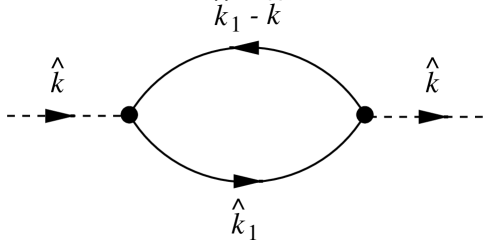
FIG. 1.: One-loop correction to the 2-point vertex function. Full lines indicate bare HRS correlators; dashed lines indicate amputated external bare HRS correlators.

Our starting point is the minimal model, Eq. (13), for which the bare correlator is given by Eq. (24). Then the one-loop correction to the 2-point vertex function comes from the diagram shown in Fig. 1, which is calculated in App. A. By choosing $\hat{k}\in 3^{+}RS$ (i.e. in the HRS but not in the two-replica sector) [32] we obtain for the inverse susceptibility $\chi^{-1}$ the result

$$(N\chi)^{-1}=-2a\tau+18g^{2}\frac{V}{N}\int\frac{d^{d}p}{(-2a\tau+bp^{2})^{2}}\,\,,$$ (36)

in which a large wavevector cut-off at $|\hat{k}|=\Lambda$ is implied. The (one-loop) shifted critical point $\tau_{\rm c}$ marks the vanishing of $\chi^{-1}$, i.e., solves

$$0=-2a\tau_{\rm c}+18g^{2}\frac{V}{N}\int\frac{d^{d}p}{(-2a\tau_{\rm c}+bp^{2})^{2}}\,\,.$$ (37)

Now, in mean-field theory the transition occurs at $\tau=0$, with positive (resp. negative) values corresponding to the amorphous solid (resp. liquid) states. From Eq. (37) we see that that inclusion of fluctuations enlarges the region of crosslink densities in which liquid state is stable, as one would expect on general physical grounds. However, it is worth noting, in passing, that without the exclusion of the one-replica sector the converse would occur (i.e. fluctuations would enlarge the region of stability of the amorphous solid state). By subtracting Eq. (37) from Eq. (36) in the standard way, replacing $\tau_{\rm c}$ by its mean-field value (of zero) in the loop correction, and rescaling the integration variable $p^{2}$ according to $bp^{2}=-2a\tau k^{2}$, we arrive at

$$(N\chi)^{-1}=-2a(\tau-\tau_{c})\left(1-18g^{2}({V}/{N})b^{-d/2}(-2a\tau)^{(d-6)/2}J_{d}\right),$$ (38)

where $J_{d}$ is a dimensionless number dependent on $d$ (and weakly on $\Lambda$, at least in regime of interest, i.e., $d$ below 6). Equation (38) shows that for $d<6$ a fluctuation dominated-regime is inevitable for sufficient small $\tau$, and hence that the upper critical dimension for the vulcanization transition is six, in agreement with naïve power-counting arguments applied to the $n\to 0$ limit of the cubic field theory, Eq. (13). The Ginzburg criterion amounts to determining the departure of $\tau$ from its critical value such that in Eq. (38) the one-loop correction is comparable in magnitude to the mean-field level result.

To determine the physical content of the Ginzburg criterion, we invoke the values of the coefficients of the minimal model appropriate for the semi-microscopic model of RCMSs, Eqs. (15)-(18), and we exchange the macromolecule density $N/V$ for the volume fraction $\varphi\equiv(N/V)(L/\ell)\ell^{d}$. Thus we arrive at the following form of the Ginzburg criterion: for $d<6$, fluctuations cannot be neglected for values of $\tau$ satisfying

$$|\tau-\tau_{\rm c}|\lesssim\left({L/{\ell}}\right)^{-\frac{d-2}{6-d}}\left({\varphi/{g^{2}}}\right)^{-\frac{2}{6-d}},$$ (39)

from which we see that the fluctuation-dominated regime is narrower for longer macromolecules and higher densities (for $2<d<6$). Such dependence on the degree of polymerization $L/\ell$ is precisely that argued for long ago by de Gennes on the basis of a percolation-theory picture [33].

Besides the fields and vertices featuring in the minimal model, there are other symmetry-allowed fields and vertices that are generated by the semi-microscopic theory of RCMSs. Examples are provided by the 1RS field, which describes density fluctuations, along with vertices of cubic, quartic or higher-order that couple the 1RS field to the HRS field. In App. B we investigate the effect of these fields and vertices, which are omitted from the minimal model, and show: (i) that the inclusion of their effects (at the one-loop level) does not change the Ginzburg criterion derived in the present section; and (ii) that the HRS critical fluctuations do not provide any singular contributions to the 1RS density-density correlation function (at least to one-loop order).

B Renormalization-group procedure and its subtleties

We now describe the RG procedure that we are using, a schematic depiction of which is given in Fig. 2. The main thrust of our approach is the standard “momentum-shell” RG, via which we aim to determine how the parameters of the theory, $\tau$ and $g$, flow under the two RG steps of coarse graining and rescaling. However, in the present context there are some significant subtleties owing to the need to constrain the fields to lie in the HRS.

In the coarse-graining step, we integrate out the rapidly-varying components of $\Omega(\hat{k})$ (i.e. those corresponding to wavevectors satisfying $\Lambda/b<|\hat{k}|<\Lambda$). Here, the constraint that only the HRS field is a critical field demands that one treat the HRS and the 1RS distinctly. We handle this by working with a large but finite (replicated) system contained in a hyper-cubic box of volume $V^{n+1}$ on which periodic boundary conditions are applied. As a consequence, the wavevectors are “quantized,” and therefore we can directly make the appropriate subtractions associated with the removal of the zero- and one-replica sectors. Having made the necessary subtractions, we compute the various Feynman diagrams (for the construction of the Ginzburg criterion and the the coarse-graining step of the RG) by passing to the continuous wavevector limit (so that wavevector summations become integrations).

The replica technique has the following curious feature. In the infinite-volume limit the different sectors are spaces of different dimensionalities, and thus the contributions from the lower replica sectors appear to be sets of measure zero relative to the contributions from the HRS. However, in the replica limit, the contributions from different sectors are comparable and, hence, the lower sectors cannot be neglected.

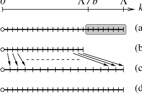
FIG. 2.: Schematic one-dimensional depiction of the basic steps of the RG procedure (the field variables are defined only at the hash marks denoting the quantized wavevectors): from (a) to (b) integrate out the fields at the quantized wavevectors $k$ in the “momentum shell”(shaded); from (b) to (c) rescale lengths to restore the wavevector cut-off, and rescale the field to restore the gradient term; from (c) to (d) restore the density of the degrees of freedom. (In practice, we employ a momentum shell of infinitesimal width.)

The coarse-graining step is followed by the rescaling step, in which the aim is to return the theory to its original form. The field- and length-rescaling aspects of this step (to recover the original wavevector cut-off and form of the gradient term) are standard, but there is a subtlety associated with the fact that the original theory is defined on a finite volume (in order that the wavevectors be quantized and the various replica sectors thereby be readily identifiable). This subtlety is that upon coarse-graining and rescaling one arrives at a theory that is almost of the original form, but is defined on a coarser lattice of quantized wavevectors associated with the reduced (real-space) volume. If we wish to return the theory to its truly original form, we are required to increase the density of the coarsened wavevector lattice. To accomplish this, we choose to make use of the extension to $(n+1)d$ dimensions of the following one-dimensional relation, exact in the thermodynamic (i.e. large real-space size $B$) limit:

$$\sum_{k\in\{2\pi nb/B\}}f(k)\approx{b}^{-1}\sum_{k\in\{2\pi n/B\}}f(k).$$ (40)

One way to understand this is to regard the two sides of Eq. (40) as providing different discrete approximations to the same continuous-wavevector (i.e. infinite-volume) limit. Thus, we expect the difference between them to be unimportant in the thermodynamic limit. Another way is to regard the right hand side of Eq. (40) as pertaining to a system with a larger number of degrees of freedom than the left hand side, but that the factor $b^{-1}$ appropriately diminishes the weight of each degree of freedom. It would be equally satisfactory if we chose, in our RG scheme, not to restore the wavevector lattice spacing, which would amount to our using the left-hand-side of Eq. (40).

C Expansion around six dimensions

In the previous two subsections we have established that the upper critical dimension for the vulcanization transition is six, and we have described an RG procedure capable of elucidating certain universal features of the transition. We now examine the RG flow equations near the upper critical dimension that emerge from this procedure, and discuss the resulting fixed-point structure and universal critical exponents. To streamline the presentation we have relegated the technical details of the derivation of the flow equations to App. C.

1 Flow equations

As with the mean-field theory and the Ginzburg criterion, our starting point is the replicated cubic field theory, Eq. (13). By suitably redefining the scales of $\Omega(\hat{k})$ and $\hat{k}$ we can absorb the coefficients $a$ and $b$, hence arriving at the Landau-Wilson effective Hamiltonian

$${\cal S}_{n}\big{(}\{\Omega\}\big{)}=N\sum_{\hat{k}\in{{\rm HRS}}}\Big{(}-\tau+\frac{1}{2}|\hat{k}|^{2}\Big{)}\big{|}\Omega(\hat{k})\big{|}^{2}-Ng\,\sum_{\hat{k}_{1},\hat{k}_{2},\hat{k}_{3}\in{{\rm HRS}}}\Omega({\hat{k}}_{1})\,\Omega({\hat{k}}_{2})\,\Omega({\hat{k}}_{3})\,\delta_{{\hat{k}_{1}}+{\hat{k}_{2}}+{\hat{k}_{3}},{\hat{0}}}\,,$$ (41)

in which all wavevector summations are cut off beyond replicated wavevectors of large magnitude $\Lambda$, from which we can read off the bare correlator

$$G_{0}(\hat{k})=\frac{1}{-2\tau+|\hat{k}|^{2}}\,\,.$$ (42)

FIG. 3.: Contributing one-loop diagrams. Full lines indicate bare HRS correlators for short-wavelength fields (i.e. fields lying in the momentum shell); wavy lines indicate long-wavelength fields.

We shall be working to one-loop order and, correspondingly, the diagrams that contribute to the renormalization of the parameters of the Landau-Wilson effective Hamiltonian are those depicted in Figs. 3 (a) and (b). The resulting flow equations are

$$d\tau/d\ln b = 2\,\tau-C_{0}\,g^{2}-C_{0}^{\prime}\,\tau\,g^{2}-C_{1}\,\tau\,g^{2}+{\cal O}(\tau^{2}g^{2},\tau{\varepsilon}g^{2},{\varepsilon}g^{2},g^{4}),$$ (44)

$$dg/d\ln b = g\big{(}{\varepsilon}/2-C_{3}g^{2}-\frac{3}{2}C_{1}g^{2}+{\cal O}(\tau g^{2},{\varepsilon}g^{2},g^{4})\big{)},$$ (45)

$$dz/d\ln b = {1\over{2}}(d+2-C_{1}g^{2})+{\cal O}(\tau g^{2},{\varepsilon}g^{2},g^{4}),$$ (46)

where ${\varepsilon}\equiv 6-d$, $b$ is the length-rescaling factor, $z$ is the field-rescaling factor, and the (constant) coefficients in the flow equations are given by

$$(C_{0},C_{0}^{\prime},C_{1},C_{3})=\frac{V}{N}\frac{S_{6}}{(2\pi)^{6}}\,(9\Lambda^{2},36,-6,72),$$ (47)

in which $S_{6}$ is the surface area of a $6$-dimensional sphere of unit radius.

2 Fixed-point analysis and its consequences

We proceed in the standard way by first finding the fixed points $(\tau_{*},g_{*})$ of the flow equations, at which $d(\tau,g)/d\ln b=(0,0)$. We linearize the flow equations about each of the resulting fixed points,

$${d\over{d\ln b}}\pmatrix{\tau-\tau_{*}\cr g-g_{*}}\approx\pmatrix{2-\big{(}C_{0}^{\prime}+C_{1}\big{)}g_{*}^{2}&-2C_{0}\,g_{*}\cr 0&\frac{1}{2}{\varepsilon}-3\big{(}C_{3}+\frac{3}{2}C_{1}\big{)}g_{*}^{2}\cr}\pmatrix{\tau-\tau_{*}\cr g-g_{*}},$$ (48)

where we have dropped higher-order corrections. We then establish the RG eigenvalues at each fixed point by finding the eigenvalues of the linearized RG transformation matrices. Finally, we solve Eq. (48) to obtain the flow near each fixed point.

For ${\varepsilon}$ both negative and positive (i.e. for $d$ both above and below six) we find a Gaussian fixed point (GFP): $(\tau_{*},g_{*})=(0,0)$. Solving Eq. (48) about this fixed point gives the flow

$$\pmatrix{\tau(b)\cr g(b)}\approx\pmatrix{\tau(1)\,b^{y_{1}}\cr g(1)\,b^{y_{2}}},$$ (49)

with the RG eigenvalues $y_{1}$ and $y_{2}$ respectively given by $y_{\tau}=2$ and $y_{g}={\varepsilon}/2$.

As one can see from Eq. (49), above six dimensions the GFP is unstable in the $\tau$ direction and stable in the $g$ direction. However, below six dimensions the GFP also becomes unstable in the $g$ direction, and a new fixed point—the Wilson-Fisher fixed point (WFFP)—emerges, located at $(\tau_{*},g_{*}^{2})=\left((\Lambda^{2}/28),(1/126)((2\pi)^{6}/S_{6})(V/N)^{-1}\right){\varepsilon}$. (Let us mention, in passing, that if we had not correctly implemented the constraint that wavevector summations exclude contributions for the 1RS then the structure of the flow equations would have been utterly different; e.g., the WFFP would have occurred at a complex value of $g$.)  By solving Eq. (48) for the WFFP we find the flow

$$\pmatrix{\tau(b)-\tau_{*}\cr g(b)-g_{*}}\approx\pmatrix{\big{(}\tau(1)-\tau_{*}\big{)}-A\big{(}g(1)-g_{*}\big{)}\cr 0}b^{y_{1}}+\pmatrix{A\big{(}g(1)-g_{*}\big{)}\cr g(1)-g_{*}}b^{y_{2}},$$ (50)

where $A\equiv\big{(}3/\sqrt{14}\big{)}\big{(}(V/N)(S_{6}/(2\pi)^{6})\big{)}^{1/2}\big{(}\Lambda^{2}{\varepsilon}^{1/2}\big{)}$ and the RG eigenvalues are given by $y_{1}=2-(5{\varepsilon}/21)$ and $y_{2}=-{\varepsilon}$.

We now proceed to obtain the critical exponents for physical quantities from the RG eigenvalues at each fixed point. The homogeneity relation for the correlator $G({\hat{k}})$, following from a standard RG analysis [34], reads

$$G({\hat{k}},\tau)=z^{2}\,b^{-d}\,G(b{\hat{k}},b^{y_{1}}\tau).$$ (51)

We eliminate $b$ by choosing $b|{\hat{k}}|=1$; then comparison with Eq. (25) leads to $\nu=1/y_{1}$ and $\eta=C_{1}g_{\ast}^{2}$. Thus, for the GFP we have

$$\nu^{-1}=2,\qquad\eta=0,$$ (52)

and for the WFFP we have, to first order in ${\varepsilon}$,

$$\nu^{-1}=2-(5{\varepsilon}/{21}),\qquad\eta=-{{\varepsilon}/{21}}.$$ (53)

Both above and below six dimensions, the critical exponents $\nu$ and $\eta$ (and $\beta$, to be discussed below) are identical to those governing analogous quantities in percolation theory (at least to first order in ${\varepsilon}$), as computed via the Potts field theory [36]. We discuss the significance of this result and the relationship between the present approach and percolation/gelation-based approaches in Sec. VI.

We have focused on the cubic interaction in the vulcanization field theory. There are, of course, additional symmetry-allowed interactions, such as the quartic interaction. Near to six dimensions, however, the fact that such interactions are irrelevant at the GFP can be shown by naïve power-counting arguments, which hold in the replica limit (and remain uncompromised at the WFFP, owing to its proximity to the GFP).

D Scaling for gel fraction and wavevector-dependent order parameter

In order to relate properties of the amorphous solid state to those computed in the liquid and critical states, we now follow the standard scaling analysis. To do this, we add to the minimal model, Eq. (41), a source field that couples linearly to the order parameter: $-N\sum_{\hat{k}\in{{\rm HRS}}}\Omega(\hat{k})\,U(-\hat{k})$. We assume that $U$ contains only long wavelength components, so that it does not couple to any field featuring in any momentum-shell integrations. Then the renormalization of $U(-{\hat{k}})$ comes only from the rescalings of $\hat{k}$ and $\Omega({\hat{k}})$, and thus we have

$$U^{\prime}({\hat{k}}^{\prime})=z\,b^{-d}\,U({\hat{k}}).$$ (54)

To obtain the exponent $\beta$, which describes the scaling of the gel fraction $q$, the conventional method prescribes the application of a uniform source field. In the present theory, the (zero replica sector) field variable $\Omega({\hat{0}})$, which would couple to such a uniform source, is excluded, and instead we choose $U({\hat{k}})=h\,\delta_{{\hat{k}}+{\hat{k}}_{0},{\hat{0}}}$, where ${\hat{k}}_{0}$ lives in the HRS but is otherwise arbitrarily small. (This prescription is consistent with the notion that the gel fraction follows from the long-wavelength limit of the order parameter, the limit being taken via wavevectors in the HRS.)  Hence we arrive the recursion relation for $h$:

$$h^{\prime}=z\,h=b^{y_{h}};\qquad y_{h}=(d+2-\eta)/2.$$ (55)

As we are already in possession of $\eta$ at the GFP and the WFFP, we thus arrive at the scaling dimension $y_{h}$ of the source field $h$.

Having obtained $y_{h}$, we now use it, together with $y_{\tau}$, $y_{g}$ and the singular part of the free energy density $f$, to determine $\beta$, in the following way. According to homogeneity, $f$ has the form

$$f(\tau,g,h)=b^{-d}f(\tau b^{y_{\tau}},gb^{y_{g}},hb^{y_{h}}).$$ (56)

By taking the derivative with respect to $h$ so as to form the order-parameter equation of state, choosing $h=0$, and passing to the small ${\hat{k}}_{0}$ limit, one finds the following scaling behavior of the gel fraction:

$$q(\tau,g,0)\sim\lim\limits_{\hat{k}_{0}\rightarrow\hat{0}}\partial f/\partial h\big{|}_{h=0}\sim b^{-d+y_{h}}\,M(\tau b^{y_{\tau}},gb^{y_{g}},0)=\tau^{{(d-y_{h})}/{y_{\tau}}}M(1,g\tau^{-y_{g}/y_{\tau}},0).$$ (57)

Let us first consider the regime $d>6$, for which the appropriate fixed point is the GFP and, therefore one expects the exponents to take on their classical values. Now, as one can see from the mean-field value for the order parameter $\overline{\Omega}$ (and thus the gel fraction $q$), Eq. (20), both of which are proportional to $g^{-1}$, the cubic interaction is dangerously irrelevant at the GFP, and thus one has

$$M(1,g,0)\sim\frac{1}{g},\quad{\rm for}\quad g\rightarrow+0.$$ (58)

Hence, near the GFP one has

$$\qquad\qquad\qquad q(\tau,g,0)\sim\tau^{\beta},\quad{\rm for}\quad g\rightarrow+0,$$ (60)

$$\qquad\qquad\qquad\beta=\frac{d-y_{h}}{y_{\tau}}+\frac{y_{g}}{y_{\tau}}=\frac{d-\frac{d+2}{2}+\frac{6-d}{2}}{2}=1,$$ (61)

which is precisely the mean-field value of the exponent $\beta$ given in Sec. III A.

Now let us turn to the regime $d<6$, for which the exponents are nonclassical. The appropriate fixed point is now the WFFP, at which the cubic interaction is irrelevant but not dangerously so. Thus, in this regime one has the standard scaling relation

$$\beta=\frac{d-y_{h}}{y_{\tau}}=1-({\varepsilon}/7),$$ (62)

where the second equality holds only to order ${\varepsilon}$.

In fact, under the (not unreasonable) assumption that there is only one characteristic length-scale in the ordered state (i.e. that the fluctuation correlation length does not provide a length-scale independent from the localization length-scale), we can go beyond the establishing of the scaling of the gel fraction (i.e. the long-wavelength limit of the order parameter) and propose a more general scaling hypothesis, which incorporates the scaling of the (singular part of the) wavevector-dependent order parameter [37]. This takes the form of the scaling hypothesis:

$$\big{\langle}\Omega(\hat{k})\big{\rangle}\propto\tau^{\beta}\,w\big{(}{\hat{k}}^{2}\tau^{2\nu}\big{)}.$$ (63)

The quantity $\tau^{\nu}$, which plays the role of the fluctuation correlation length in the liquid state, is here seen to play the role of the characteristic scale for the localization lengths in the ordered state. Presumably, it also governs the scale over which (amplitude-type) fluctuations are correlated in the solid state. Let us note that the mean-field result for the order parameter not only obeys this scaling relation (with $\beta=2\nu=1$) but also provides an explicit form for the function $w$.

VI Concluding remarks: Connections with other approaches and the role of thermal fluctuations

Having constructed an RG theory for the liquid and critical states of vulcanized matter, we now examine the results of this RG theory and discuss the relationship between these results and the results of other approaches to the vulcanization transition. As we have seen in Secs. V C, via an expansion around six spatial dimensions our minimal model for the vulcanization transition yields values for certain critical exponents that characterize the behavior of the system near to and at the transition. These exponents turn out to be numerically equal to those characterizing physically analogous quantities in percolation theory, at least to first order in the departure ${\varepsilon}$ from six dimensions. We have not proven that the equality between exponents holds beyond first order in ${\varepsilon}$, although there are hints in the structure of the theory suggesting that it does.

This equality between exponents seems reasonable in view of the intimate relationship between percolation theory and the connectivity of the system of crosslinked macromolecules, this connectivity pertaining to the statistics of systems formed according to the Deam-Edwards distribution of quenched randomness (and hence to the statistical mechanics of the uncrosslinked macromolecular liquid) [38]. Indeed, a connection between the percolation and vulcanization transitions already shows up at the level of mean-field theory: the dependence of the gel fraction $q$ on the crosslink-density control parameter $\mu^{2}$ obtained via the semi-microscopic approach (in the case of RCMSs), viz., that $q$ obeys

$$1-q=\exp\left(-\mu^{2}q\right),$$ (64)

is identical to the mean-field–percolation dependence of the fraction of sites participating in the infinite cluster, obtained by Erdős and Rényi in their work on random graphs [39], this identity holding not just near the transition, where the dependence of $q$ on $\mu^{2}-\mu_{\rm c}^{2}$ is linear, but for all crosslink densities. Moreover, the mean-field result emerging from the minimal model of the vulcanization transition yields this linear dependence (but cannot, of course, be applied beyond the transition regime). The relevance of percolation theory to the vulcanization transition also manifests itself beyond the mean-field level in the physical meaning of the order-parameter correlator, as we have discussed in Sec. IV. This connection has long been realized, and supports the use of percolative approaches as models of certain aspects of the vulcanization transition [16, 17, 18, 19, 20].

These percolative approaches include direct applications of percolation theory [16, 17, 18, 19], mentioned in the preceding paragraph, as well as the approach given by Lubensky and Isaacson [20]. The latter approach extends the connection between the statistics of linear macromolecules and the zero-component limit of a spin system [41, 42]. In this way, a correspondence is established between the statistics of branched, polydisperse, macromolecules and a multi-component field theory. This field theory reduces to the one-state limit of the Potts model under circumstances appropriate for the transition to a physical gel (i.e. a state in which one is certain to find a reversibly-bonded, infinite, branched macromolecule) [43].

An essential ingredient of the approaches discussed in the previous paragraph is the Potts model in its one-state limit—a representation of percolation [44, 45]. It is therefore worth considering similarities and differences between the minimal field theory of the vulcanization transition focused on in the present Paper, Eq. (13), and the minimal field theory for the Potts model. The minimal field theory for the Potts model is the $n\to 0$ limit of the cubic $(n+1)$-component field theory, the Landau-Wilson Hamiltonian for which is

$$\int_{V}d^{d}x\,\Big{(}\,\sum_{\alpha=1}^{n}\left({1\over{2}}r\,\psi_{\alpha}^{2}+{1\over{2}}|\nabla\psi_{\alpha}|^{2}\right)-w^{(3)}\sum_{\alpha,\beta,\gamma=1}^{n}\lambda^{(3)}_{\alpha\beta\gamma}\,\psi_{\alpha}\,\psi_{\beta}\,\psi_{\gamma}\Big{)},$$ (65)

where $r$ controls the bond-occupation probability (and hence the percolation transition), $w^{(3)}$ is the nonlinear coupling strength, and $\lambda^{(3)}_{\alpha\beta\gamma}$ is the “Potts tensor” (which controls the internal symmetry of the theory; for a discussion of this theory see, e.g., Sec. 2.7 of Ref. [21]).

How does this Potts field theory compare the vulcanization field theory that we have been analyzing in the present Paper? The Potts field theory has, a cubic interaction, as does the vulcanization field theory, and therefore its upper critical dimension is also six. If we examine the RG analysis of the Potts field theory (in an expansion around six dimensions) [46] we see that, at the one-loop level, diagrams identical in form (i.e. those shown in Fig. 3) enter the renormalization of the various vertices. Moreover, in the $n\to 0$ limit the RG flow equations for the two theories turn out to be identical. This striking result is connected to the following observations: (i) In Potts case, aside from the $d$-dimensional integrals corresponding to the diagrams, the coefficients in the flow equations are determined by the contractions of Potts-tensor indices associated with each cubic vertex, these contractions being the origin of the $n$-dependence of the coefficients in the flow equations. (ii) In the vulcanization case, the diagrams intrinsically correspond to $(n+1)d$-dimensional integrals but, due to the constraints on the summations over wavevectors, these diagrams produce $(n+1)d$-dimensional integrals (which smoothly reduces to $d$-dimensional integrals in the $n\to 0$ limit), together with $d$-dimensional integrals [see Eqs. (A2,C26)]. (iii) Despite the explicit differences in the forms of the two theories, it turns out that, in the $n\to 0$ limit, the integrals and the combinatorics conspire to produce precisely the same flow equations. In some delicate way, which we do not fully understand, the constraints on the wavevector summations in the vulcanization theory play a similar role to the field-index contractions in the Potts theory.

Having discussed the similarities of the Potts and vulcanization approaches, let us now catalogue the many distinctions between them: (i) The Potts field theory has a multiplet of $n$ real fields on $d$-dimensional space; the vulcanization field theory has a real singlet field living on $(n+1)$-fold replicated $d$-dimensional space. (ii)  The Potts field theory represents a setting involving a single ensemble [22], the ensemble of percolation configurations, whereas the vulcanization field theory describes a physical problem in which two distinct ensembles (thermal and disorder) play essential roles. As such, the vulcanization field theory is capable of providing a unified theory not only of the transition but also of the structure, correlations and (e.g. elastic) response of the emerging amorphous solid state. This is already manifested at the mean-field level, inasmuch as the vulcanization field theory presents an order parameter that is far richer in its physical content that the one presented by the Potts model. (iii) The entire symmetry structures possessed by the percolation and vulcanization field theories are quite different. The Potts field theory has translational and rotational invariance (in unreplicated space), along with the discrete symmetry of $(n+1)$-fold permutations of the field components. The vulcanization field theory has the symmetries of the independent translations and rotations of the $(n+1)$ replicas of space, along with the discrete symmetry of $(n+1)$-fold permutations amongst the replicas. (iv) The nature of the spontaneous symmetry breaking at the percolation and vulcanization phase transitions is distinct. The percolation transition (in its Potts representation) involves the spontaneous breaking of the ($n\to 0$ limit) of a discrete $(n+1)$-fold permutation symmetry. By contrast, the vulcanization transition involves the spontaneous breaking of the ($n\to 0$ limit of the) continuous symmetry of relative translations and rotations of the $n+1$ replicas; the permutation symmetry remains intact in the amorphous solid state, as does the symmetry of common translations and rotations of replicated space. Thus, the vulcanization transition is associated with the appearance of low-energy, long-wavelength, Goldstone-type excitations [28], which we expect to lead to the restoration of the broken continuous symmetry in and below a lower critical dimension of two. By contrast, fluctuations destroy the percolation transition only at and below the the lower critical dimension of unity.

Whilst there are these apparent distinctions between the percolation and vulcanization approaches, especially in low dimensions, there is also evidence in favor of some sort of sharp correspondence between the physics of percolation and vulcanization coming from the computation of critical exponents near the upper critical dimension. This apparent dichotomy can, however, be reconciled if we carefully delineate between three logically distinct physical properties pertaining to RCMSs and other randomly constrained systems: (i) macroscopic network formation (by which we mean that constraints are present in sufficient density to connect a nonzero fraction of the constituents into a giant random molecule); (ii) random localization (by which we mean the change in thermal motion of a nonzero fraction of the constituents from wandering throughout the container to fluctuating only over finite distances from their random mean positions); and (iii) the acquisition of rigidity (by which we mean the emergence of a nonzero static shear modulus). Within mean-field theory (and hence above six spatial dimensions), these three properties go hand in hand, emerging simultaneously at the phase transition. At and below six dimensions they appear to continue to go hand in hand (although, strictly speaking, we have not yet investigated the issue of the acquisition of rigidity beyond mean-field theory)  until one reaches two dimensions where we believe this broad picture will change (as we shall discuss shortly). Thus, it appears that, within the limited sphere of issues concerning amorphous solidification that percolation-based approaches are capable of addressing, such approaches do not lead one astray. In other words, the superposition of thermal fluctuations on the positions of the constituents of the macroscopic network that emerges as the constraint density is increased towards the phase transition does not lead to any changes in the critical exponents governing percolation-type quantities: disorder fluctuations appear to play a more important role than do thermal fluctuations, as far as the percolative aspects of the critical phenomenon are concerned.

This brings up the interesting issue of the nature of the vulcanization transition and its relationship with the percolation transition as the dimensionality of space is reduced to the neighborhood of two spatial dimensions, two being the lower critical dimension of the vulcanization transition. (The ideas reported in this paragraph result from an ongoing collaboration with H. E. Castillo [47].)  Indeed, the case of two dimensions is especially fascinating in view of the fact that there is a conventional percolation transition in two dimensions, whereas the thermal fluctuations are expected to be sufficiently prominent to destablize the amorphous solid phase, in which case the macroscopic network formation no longer occurs simultaneously with the random localization of constituents of the network. It is tempting to speculate [47] that in two dimensions an anomalous type of vulcanization transition (not accompanied by true localization) continues to happen simultaneously with percolation transition. As the constraint density is tuned from below to above criticality, the amorphous solidification order parameter would remain zero, whereas the order-parameter correlations would change from decaying exponentially to decaying algebraically with distance. One might say that (constraint-density controlled) cluster fragmentation (rather than the thermal excitation of lattice defects, as in regular two-dimensional melting) would be mediating the melting transition. If this scenario should happen to be borne out then, at sufficiently high crosslink densities one would have a quasi-amorphous solid state—the random analogue of a two-dimensional solid [48]—exhibiting quasi-long-range positional order but of a random rather than regular type. By implementing these ideas via an effective field theory that describes low-energy excitations of the amorphous solid state, we hope to construct a picture of the vulcanization transition and the emergent rigid state in and near two spatial dimensions. Such a development would complement the approach to the vulcanization transition, presented here, which is based on expanding about the upper critical dimension, e.g., by providing access to critical exponents via an expansion about two rather than six dimensions.

A Inverse susceptibility and Ginzburg criterion

In order to calculate the one-loop correction to the 2-point vertex function ${\Gamma}^{(2)}(\hat{k})$, we first calculate the self-energy $\Sigma_{n}(\hat{k})$ (i.e. the sum of all two-point one-particle-irreducible amputated diagrams), in terms of which ${\Gamma}^{(2)}(\hat{k})\equiv G_{0}(\hat{k})^{-1}-\Sigma_{n}(\hat{k}){\big{|}}_{n\to 0}$. To one-loop order, $\Sigma_{n}(\hat{k})$ is given by the amputated diagram shown in Fig. 1,

$$\Sigma_{n}(\hat{k})=18g^{2}\sum_{\hat{k}_{1}\in{\rm HRS}\atop(\hat{k}-\hat{k}_{1}\in{\rm HRS})}G_{0}(\hat{k}_{1})\,G_{0}(\hat{k}_{1}-\hat{k}).$$ (A1)

Let us emphasize the meaning of the notation: one is directed to sum over all replicated wavevectors $\hat{k}_{1}\in{\rm HRS}$ subject to the constraint that $\hat{k}-\hat{k}_{1}\in{\rm HRS}$; one should also bear in mind the fact that the external wavevector $\hat{k}$ lies in the HRS. This constrained summation can be expressed in terms of several unconstrained summations (for cases in which $\hat{k}$ has nonzero entries in at least three replicas, i.e., lies in the $3^{+}$RS) as

$$\sum_{\hat{k}_{1}\in{\rm HRS}\atop(\hat{k}-\hat{k}_{1}\in{\rm HRS})}O(\hat{k}_{1})=\sum_{\hat{k}_{1}}O(\hat{k}_{1})-\sum_{\alpha=0}^{n}\sum_{{\bf p}}O(\hat{k}_{1})\Big{|}_{\hat{k}_{1}={\bf p}\hat{e}^{\alpha}}+nO(\hat{k}_{1})\Big{|}_{\hat{k}_{1}=\hat{0}}-\sum_{\alpha=0}^{n}\sum_{{\bf p}}O(\hat{k}_{1})\Big{|}_{\hat{k}_{1}={\bf p}\hat{e}^{\alpha}+\hat{k}}+nO(\hat{k}_{1})\Big{|}_{\hat{k}_{1}=\hat{k}}\,\,\,,$$ (A2)

for any $O(\hat{k}_{1})$. Here, $\{\hat{e}^{\alpha}\}_{\alpha=0}^{n}$ is the collection of unit vectors in replicated space, so that, e.g., a generic vector $\hat{p}$ can be expressed as $\sum_{\alpha=0}^{n}{\bf p}^{\alpha}\hat{e}^{\alpha}$. When $\hat{k}$ belongs to the 2RS [e.g. $\hat{k}=({\bf l}^{1},{\bf l}^{2},{\bf 0},\cdots,{\bf 0})$] there is a slight modification of Eq. (A2) and, instead, we have

$$\sum_{\hat{k}_{1}\in{\rm HRS}\atop(\hat{k}-\hat{k}_{1}\in{\rm HRS})}O(\hat{k}_{1}) = \sum_{\hat{k}_{1}}O(\hat{k}_{1})-\sum_{\alpha=0}^{n}\sum_{{\bf p}}O(\hat{k}_{1})\Big{|}_{\hat{k}_{1}={\bf p}\hat{e}^{\alpha}}+nO(\hat{k}_{1})\Big{|}_{\hat{k}_{1}=\hat{0}}-\sum_{\alpha=0}^{n}\sum_{{\bf p}}O(\hat{k}_{1})\Big{|}_{\hat{k}_{1}={\bf p}\hat{e}^{\alpha}+\hat{k}}$$ (A4)

$$\qquad\qquad\qquad\quad+\,nO(\hat{k}_{1})\Big{|}_{\hat{k}_{1}=\hat{k}}+O(\hat{k}_{1})\Big{|}_{\hat{k}_{1}={\bf l}^{1}\hat{e}^{1}}+O(\hat{k}_{1})\Big{|}_{\hat{k}_{1}={\bf l}^{2}\hat{e}^{2}}\,\,.$$

For the moment, let us focus on the case of $\hat{k}\in 3^{+}$RS. By making use of Eq. (A2), and subsequently transforming each unconstrained summation into an integral, we obtain

$$\Sigma_{n}(\hat{k})=18g^{2}\Big{(}V^{n+1}\int d^{(n+1)d}k_{1}\,G_{0}(\hat{k}_{1})\,G_{0}(\hat{k}_{1}-\hat{k})-2\sum_{\alpha=0}^{n}V\int d^{d}p\,G_{0}({\bf p}\hat{e}^{\alpha})\,G_{0}({\bf p}\hat{e}^{\alpha}-\hat{k})+2n\,G_{0}(\hat{0})\,G_{0}(\hat{k})\Big{)}.$$ (A5)

The limit of the validity of the Landau theory (i.e. the tree-level approximation) can be ascertained by enquiring when the loop corrections to the inverse susceptibility become comparable its tree-level value. Thus we take the long-wavelength limit of the correction (A1) via a sequence of wavevectors $\hat{k}$ lying in the HRS, obtaining

$$\Sigma_{n}(\hat{k})\big{|}_{\hat{k}\rightarrow\hat{0}}=18g^{2}\Big{(}V^{n+1}\int d^{(n+1)d}k_{1}\,{G_{0}}(\hat{k}_{1})^{2}-2(n+1)V\int d^{d}p\,{G_{0}}({\bf p})^{2}+2n{G_{0}}(\hat{0})^{2}\Big{)}.$$ (A6)

At this stage, the $n\rightarrow 0$ limit may be taken [the reason for this is discussed in Sec. II D, shortly after Eq. (13)]. In addition, the integral over the $(n+1)$-fold replicated space goes smoothly into an integral over the ordinary (i.e. unreplicated) space. Thus, we arrive at

$$\Sigma(\hat{k})\big{|}_{\hat{k}\rightarrow\hat{0}}\equiv\lim_{n\rightarrow 0}\Sigma_{n}(\hat{k})\big{|}_{\hat{k}\rightarrow\hat{0}}=18g^{2}\Big{(}V\int d^{d}p\,{G_{0}}({\bf p})^{2}-2V\int d^{d}p\,{G_{0}}({\bf p})^{2}\Big{)}.$$ (A7)

From this expression, we see an example of what turns out to be a typical effect of the exclusion of the 1RS, viz., that it reverses the sign relative to the unconstrained version. By collecting this loop correction together with the tree-level inverse susceptibility, we arrive at the result that we shall use to establish the Ginzburg criterion:

$$(N\chi)^{-1}\equiv N^{-1}{\Gamma}^{(2)}(\hat{k})\big{|}_{\hat{k}\rightarrow\hat{0}}={G_{0}}(\hat{0})^{-1}-N^{-1}\Sigma(\hat{k})\big{|}_{\hat{k}\rightarrow\hat{0}}=-2a\tau+18g^{2}{V\over{N}}\int\frac{d^{d}p}{(-2a\tau+bp^{2})^{2}}\,\,.$$ (A8)

We mention, in passing, that when $\hat{k}$ lies in the 2RS, we need to use Eq. (A4) instead of Eq. (A2) in evaluating the constrained summation. The resulting two extra terms in $\chi^{-1}$ turn out to be nonextensive and non-divergent at the transition, and thus do not change the result for the Ginzburg criterion. (The appearance of non-extensive terms may seem strange, but also occurs in the semi-microscopic theory of RCMSs, where the free energy for the saddle point value of the order parameter has a non-extensive part; for a discussion of this issue see Sec. 2.6 of Ref. [4].)

B Subleading elements: Additional semi-microscopically generated fields and vertices

The inspiration for the minimal model, Eq. (13), discussed in Sec. II D, comes from experience with detailed statistical-mechanical investigations of various semi-microscopic models of RCMSs and related systems [3, 4, 11, 12]. The field theories obtained in these investigations contain additional fields and vertices beyond those featuring in the minimal model. Amongst them are: the 1RS field [variously denoted as $\Omega({\bf k}\hat{e}^{\alpha})$ or $\Omega^{\alpha}({\bf k})$], which describes density fluctuations; various vertices that couple the 1RS field to itself and to the HRS field; and quartic or higher-order HRS vertices. In the present section we discuss the role of these additional fields and vertices. We shall confine our attention to effects that show up at the one-loop level. To avoid confusion we shall, in this section, denote the bare HRS and 1RS correlators respectively by $G_{0}^{\rm HRS}$ and $G_{0}^{\rm 1RS}$.

FIG. 4.: Example of a one-loop correction to the self-energy due to a vertex omitted from the minimal model.

1 Subleading influences on the higher replica sector

We begin by considering the possible corrections to the HRS self-energy $\Sigma_{n}(\hat{k})|_{{\hat{k}}\to{\hat{0}}}$ arising from the additional fields and vertices. At the one-loop level, the only contributions arising from an omitted vertex are those associated with the quartic vertex, for which there are two situations to consider, depending on whether the loop wavevector lies in the 1RS or the HRS. Figure 4 shows the relevant diagram.

Let us first look at the contribution of this diagram when the loop wavevector lies in the HRS. In this case, evaluating the diagram involves the constrained summation:

$$\sum_{\hat{k}\in{{\rm HRS}}}G_{0}^{\rm HRS}(\hat{k}) = \sum_{\hat{k}}G_{0}^{\rm HRS}(\hat{k})-\sum_{\alpha=0}^{n}\sum_{{\bf k}}G_{0}^{\rm HRS}({\bf k}\hat{e}^{\alpha})+nG_{0}^{\rm HRS}(\hat{0})$$ (B1)

$$= \sum_{\hat{k}}G_{0}^{\rm HRS}(\hat{k})-(n+1)\sum_{{\bf k}}G_{0}^{\rm HRS}({\bf k})+nG_{0}^{\rm HRS}(\hat{0}),$$ (B2)

which vanishes in the $n\rightarrow 0$ limit.

Let us now look at the contribution of this diagram when the loop wavevector lies in the 1RS. In this case, no critical bare correlators feature, so that the resulting contribution to $\Sigma_{n}(\hat{k})|_{{\hat{k}}\to{\hat{0}}}$ is finite. There are also contributions to $\Sigma_{n}(\hat{k})|_{{\hat{k}}\to{\hat{0}}}$ arising from one-loop diagrams involving two cubic vertices, in which either one or both loop-wavevectors lie in the 1RS. None of these contributions alters the Ginzburg criterion established in Sec. V A.

2 Absence of feedback of critical fluctuations on the density-density correlator

As we have discussed in Sec. III, the 1RS field $\Omega({\bf k}\hat{e}^{\alpha})$, which describes density fluctuations, remains “massive” at the vulcanization transition (i.e. the coefficient of the term quadratic in this field remains positive at the transition), and the corresponding bare correlator is nonsingular at the vulcanization transition. We now examine the effects of HRS critical fluctuations on the correlator of the 1RS field. We approach this issue by studying those one-loop diagrams for the 1RS self-energy in which at least one internal wavevector lies in the HRS; there are three types of contribution to consider: (i) There is the contribution associated with the diagram shown in Fig. 4 but with the external wavevectors now lying in the 1RS. By the same reasoning that we applied to Eq. (B2), this contribution vanishes in the $n\rightarrow 0$ limit. (ii) There are the two contributions associated with the type of diagram shown in Fig. 1. When one of the internal wavevectors lies in the 1RS and the other lies in the HRS, the contribution involves a constrained summation over $\hat{k}$ with $\hat{k}\in{{\rm HRS}}$ and $({\bf p}\hat{e}^{\alpha}-\hat{k})\in{\rm 1RS}$ (where $\hat{k}$ is the loop wavevector and ${\bf p}\hat{e}^{\alpha}$ is the external wavevector). In this case, the constraints on the summation require that $\hat{k}\in 2$RS and $\hat{k}={\bf p}\hat{e}^{\alpha}+{\bf l}\hat{e}^{\beta}$, where $\beta\neq\alpha$ and ${\bf l}\neq{\bf 0}$. Then, the contribution to the 1RS self-energy reads

$$\sum_{\hat{k}\in{\rm HRS}\atop({\bf p}\hat{e}^{\alpha}-\hat{k}\in{\rm 1RS})}G_{0}^{\rm HRS}(\hat{k})\,G_{0}^{\rm 1RS}({\bf p}\hat{e}^{\alpha}-\hat{k}) = \sum_{\beta(\neq\alpha)}\sum_{{\bf l}\neq{\bf 0}}G_{0}^{\rm HRS}({\bf p}\hat{e}^{\alpha}+{\bf l}\hat{e}^{\beta})\,G_{0}^{\rm 1RS}(-{\bf l}\hat{e}^{\beta})$$ (B3)

$$= n\sum_{{\bf l}\neq{\bf 0}}G_{0}^{\rm HRS}({\bf p}\hat{e}^{\alpha}+{\bf l}\hat{e}^{\beta})\,G_{0}^{\rm 1RS}(-{\bf l}\hat{e}^{\beta})|_{\beta\neq\alpha}\,\,,$$ (B4)

which evidently vanishes in the $n\rightarrow 0$ limit. On the other hand, when both internal wavevectors lie in the HRS, the contribution involves the constrained summation over $\hat{k}$ with $\hat{k}\in{{\rm HRS}}$ and $({\bf p}\hat{e}^{\alpha}-\hat{k})\in{{\rm HRS}}$. In this case, the contribution to the 1RS self-energy reads

$$\sum_{\hat{k}\in{\rm HRS}\atop({\bf p}\hat{e}^{\alpha}-\hat{k}\in{\rm HRS})}\!\!\!\!G_{0}^{\rm HRS}(\hat{k})\,G_{0}^{\rm HRS}({\bf p}\hat{e}^{\alpha}-\hat{k})=\sum_{\hat{k}\in{{\rm HRS}}}\!\!G_{0}^{\rm HRS}(\hat{k})\,G_{0}^{\rm HRS}({\bf p}\hat{e}^{\alpha}-\hat{k})-\!\!\sum_{\hat{k}\in{\rm HRS}\atop({\bf p}\hat{e}^{\alpha}-\hat{k}\in{\rm 1RS})}\!\!\!\!G_{0}^{\rm HRS}(\hat{k})\,G_{0}^{\rm HRS}({\bf p}\hat{e}^{\alpha}-\hat{k})\propto n\,,$$ (B5)

which also evidently vanishes in the $n\rightarrow 0$ limit. [In the last step we have used Eq. (B4), as well the strategy for handling constrained summations employed in Eq. (B2).]

We conclude that, to one-loop order, the 1RS self-energy does not acquire any singular contributions due to critical fluctuations in the HRS. In this sense, the two sectors are well separated in the neighborhood of the vulcanization transition. However, it is straightforward to show [49] that there are 1RS correlators, such as those involving four 1RS fields but only two replica indices, which do become long ranged at the vulcanization transition and are thus capable of signaling the transition.

C Derivation of flow equations within the epsilon expansion

1 Implementation of the momentum-shell RG

The first step in the momentum-shell RG approach that we are adopting is to integrate out Fourier components of the field $\Omega(\hat{k})$ having wavevectors in the shell $\Lambda/b<|\hat{k}|<\Lambda$. To do this, we define $\Omega^{<}$ and $\Omega^{>}$, respectively the long and short wavelength components of $\Omega(\hat{k})$, by

$$\Omega^{<}({\hat{k}}) = \cases{0,&for $\Lambda/b<|\hat{k}|<\Lambda$;\cr\Omega(\hat{k}),&for \phantom{$/b\,$}$0<|\hat{k}|<\Lambda/b$;}$$ (C2)

$$\Omega^{>}({\hat{k}}) = \cases{\Omega(\hat{k}),&for $\Lambda/b<|\hat{k}|<\Lambda$;\cr 0,&for \phantom{$/b\,$}$0<|\hat{k}|<\Lambda/b$.}$$ (C3)

Then, by exchanging $\Omega(\hat{k})$ for $\Omega^{>}({\hat{k}})$ and $\Omega^{<}({\hat{k}})$ in Eq. (41) we can re-express the effective Hamiltonian as

$${\cal S}_{n}\big{(}\{\Omega\}\big{)} = {\cal S}_{n}\big{(}\{\Omega^{<}\}\big{)}+N\sum_{\hat{k}\in{{\rm HRS}}}\Big{(}-\tau+\frac{1}{2}|\hat{k}|^{2}\Big{)}\big{|}\Omega^{>}({\hat{k}})\big{|}^{2}-V\big{(}\{\Omega\}\big{)},$$ (C5)

$$V\big{(}\{\Omega\}\big{)} \equiv Ng\,\sum_{\hat{k}_{1},\hat{k}_{2},\hat{k}_{3}\in{{\rm HRS}}}\,\delta_{{\hat{k}_{1}}+{\hat{k}_{2}}+{\hat{k}_{3}},{\hat{0}}}\Big{(}\Omega^{>}({\hat{k}}_{1})\,\Omega^{>}({\hat{k}}_{2})\,\Omega^{>}({\hat{k}}_{3})$$ (C7)

$$\qquad+\,3\Omega^{<}({\hat{k}}_{1})\,\Omega^{>}({\hat{k}}_{2})\,\Omega^{>}({\hat{k}}_{3})+3\Omega^{<}({\hat{k}}_{1})\,\Omega^{<}({\hat{k}}_{2})\,\Omega^{>}({\hat{k}}_{3})\Big{)}\,.$$

Now, focusing on the partition function, we integrate out the aforementioned short-wavelength field components $\Omega^{>}$ in the context of a cumulant expansion in $V$. Thus, Eq. (12) becomes

$$[Z^{n}] \,\propto\int{{\overline{\cal D}}^{\dagger}}\Omega^{<}\,\exp\big{(}-{\cal S}_{n}^{<,{\rm eff}}),$$ (C9)

$${\cal S}_{n}^{<,{\rm eff}}\big{(}\{\Omega^{<}\}\big{)} \,\equiv{\cal S}_{n}\big{(}\{\Omega^{<}\}\big{)}-\ln\big{\langle}\exp V\big{\rangle}_{>}\,,$$ (C10)

$$\ln\big{\langle}\exp V\big{\rangle}_{>} \,\equiv\ln\left\{{\displaystyle\int{{\overline{\cal D}}^{\dagger}}\Omega^{>}\,\exp\Big{(}-N\sum\nolimits_{\hat{k}\in{{\rm HRS}}}\big{(}-\tau+\frac{1}{2}|\hat{k}|^{2}\big{)}\big{|}\Omega^{>}({\hat{k}})\big{|}^{2}\Big{)}\,\exp V\over{\displaystyle\int{{\overline{\cal D}}^{\dagger}}\Omega^{>}\,\exp\Big{(}-N\sum\nolimits_{\hat{k}\in{{\rm HRS}}}\big{(}-\tau+\frac{1}{2}|\hat{k}|^{2}\big{)}\big{|}\Omega^{>}({\hat{k}})\big{|}^{2}\Big{)}}}\right\}$$ (C12)

$$\approx\big{\langle}V\big{\rangle}_{>}+\frac{1}{2!}\Big{(}\big{\langle}V^{2}\big{\rangle}_{>}-\big{\langle}V\big{\rangle}_{>}^{2}\Big{)}+\frac{1}{3!}\Big{(}\big{\langle}V^{3}\big{\rangle}_{>}-3\big{\langle}V\big{\rangle}_{>}\big{\langle}V^{2}\big{\rangle}_{>}+2\big{\langle}V\big{\rangle}_{>}^{3}\Big{)}+{\cal O}(V^{4}).$$

Note that we have not explicitly given the factor associated with Gaussian fluctuations in the wavevector shell because it is nonsingular and, therefore, does not contribute to the quantities that we are focusing on, viz., the RG flow equations.

Next, we calculate ${\cal S}_{n}^{<,{\rm eff}}$ to the one-loop level by computing the cumulant expansion to ${\cal O}(V^{3})$ and discarding operators that are irrelevant in the vicinity of $d=6$. This amounts to retaining only terms of the form of those present in the original minimal model, and thus we are in a position to begin the task of recasting the resulting theory in its original form. The terms that must be considered correspond to the diagrams shown in Fig. 3, and are computed in Sec. C 2. When included, they produce the following intermediate form for the effective coarse-grained Hamiltonian:

$${\cal S}_{n}^{<,{\rm eff}}={\cal S}_{n}^{<}-\sum_{\hat{k}\in{{\rm HRS}}}f_{2}(\hat{k})\,\big{|}\Omega^{<}({\hat{k}})\big{|}^{2}-\sum_{\hat{k}_{1},\hat{k}_{2},\hat{k}_{3}\in{{\rm HRS}}}f_{3}(\hat{k}_{1},\hat{k}_{2},\hat{k}_{3})\,\Omega^{<}({\hat{k}}_{1})\,\Omega^{<}({\hat{k}}_{2})\,\Omega^{<}({\hat{k}}_{3})\,\delta_{{\hat{k}_{1}}+{\hat{k}_{2}}+{\hat{k}_{3}},{\hat{0}}}\,,$$ (C13)

where the functions $f_{2}$ and $f_{3}$ can be found in Sec. C 2. In fact, only their long wavelength parts are needed, i.e., we shall only need the constants $f_{2}^{(0)}$, $f_{2}^{(1)}$ and $f_{3}^{(0)}$ in the Taylor expansions

$$f_{2}(\hat{k}) \approx f_{2}^{(0)}+\frac{1}{2}f_{2}^{(1)}|\hat{k}|^{2}+{\cal O}(\hat{k}^{4}),$$ (C15)

$$f_{3}(\hat{k}_{1},\hat{k}_{2},\hat{k}_{3}) \approx f_{3}^{(0)}+{\cal O}(\hat{k}_{1}^{2},\hat{k}_{2}^{2},\hat{k}_{3}^{2},\hat{k}_{1}\cdot\hat{k}_{2},\hat{k}_{1}\cdot\hat{k}_{3},\hat{k}_{2}\cdot\hat{k}_{3}).$$ (C16)

The next step is to rescale $\Omega^{<}$ and $\hat{k}$ via

$$\Omega^{<}({\hat{k}}) = z\,\Omega^{\prime}({\hat{k}}^{\prime}),$$ (C18)

$${\hat{k}}^{\prime} = b\,{\hat{k}}.$$ (C19)

The recasting of the theory in its original form also involves the restoration of the wavevector lattice, as discussed in Sec. V B. Having made this restoration, we arrive at recursion relations for $\tau$ and $g$, along with the condition that the coefficient of the gradient term be restored to its original value:

$$\tau^{\prime} = \big{(}\tau+f_{2}^{(0)}/N\big{)}z^{2}b^{-(n+1)d},$$ (C21)

$$g^{\prime} = \big{(}g+f_{3}^{(0)}/N\big{)}z^{3}b^{-2(n+1)d},$$ (C22)

$$1 = \big{(}1-f_{2}^{(1)}/N\big{)}z^{2}b^{-(n+1)d-2}.$$ (C23)

The computation of the coefficients in the recursion relations simplifies under the convenient choice of $b=1+x$ with $x$ positive and very small, because it allows the approximation of the shell integrals by the product of end-point values of the integrands and the shell volumes. Thus, we arrive at the differential RG recursion relations (i.e. flow equations) given in the main text in Eqs. (44) and (45), along with the coefficients (47).

2 Evaluation of two diagrams

The renormalizations of $\tau$ and the gradient term acquire a nontrivial contribution associated with diagram (a) of Fig. 3, which determines $f_{2}(\hat{k})$ in Eq. (C13). Thus, including the symmetry factor of the diagram, we need to evaluate

$$f_{2}(\hat{k})=9g^{2}\sum_{\hat{k}_{1}\in{{\rm HRS}}\atop(\hat{k}_{1}-\hat{k}\in{{\rm HRS}})}G_{0}(\hat{k_{1}})\,G_{0}(\hat{k}_{1}-\hat{k}).$$ (C24)

We have encountered this kind of constrained summation in App. A, and we use the recipe given there, together with the facts that the external wavevector satisfies $|\hat{k}|\in(0,\Lambda/b)$ whereas the internal wavevectors satisfy $|\hat{k}_{1}|\in(\Lambda/b,\Lambda)$ and $|\hat{k}_{1}-\hat{k}|\in(\Lambda/b,\Lambda)$. In practice, we are concerned with the small-$\hat{k}$ behavior of $f_{2}(\hat{k})$, in which case the latter two constraints are equivalent (the difference in their effects being sub-dominant). Thus, by invoking Eq. (A2) we arrive at

$$f_{2}(\hat{k})=9g^{2}\left(\frac{V^{n+1}}{{(2\pi)}^{(n+1)d}}\int\limits_{{\Lambda/b}<|\hat{k}|<{\Lambda}}d^{(n+1)d}k_{1}\,G_{0}(\hat{k_{1}})\,G_{0}(\hat{k}_{1}-\hat{k})\right.$$ (C25)

$$\qquad\qquad\qquad\qquad\left.-2\sum_{\alpha=0}^{n}\frac{V}{{(2\pi)}^{d}}\int\limits_{{\Lambda/b}<|{\bf p}|<{\Lambda}}d^{d}p\,G_{0}({\bf p}\hat{e}^{\alpha})\,G_{0}({\bf p}\hat{e}^{\alpha}-\hat{k})\right).$$ (C26)

Then, by expanding for small $\hat{k}$ and taking the $n\rightarrow 0$ limit, we obtain

$$f_{2}^{(0)} = -\frac{9}{4}g^{2}V\frac{S_{d}}{(2\pi)^{d}}\int_{\Lambda/b}^{\Lambda}\frac{k^{d-1}dk}{(-\tau+k^{2}/2)^{2}}+{\cal O}(g^{4}),$$ (C28)

$$f_{2}^{(1)} = -\frac{9}{4}g^{2}V\frac{S_{d}}{(2\pi)^{d}}\bigg{(}-\int_{\Lambda/b}^{\Lambda}\frac{k^{d-1}dk}{(-\tau+k^{2}/2)^{3}}+{2\over{d}}\int_{\Lambda/b}^{\Lambda}\frac{k^{d+1}dk}{(-\tau+k^{2}/2)^{4}}\bigg{)}+{\cal O}(g^{4}),$$ (C29)

where $S_{d}$ is the surface area of a $d$-dimensional sphere of unit radius.

The renormalization of $g$ acquires a nontrivial contribution associated with diagram (b) of Fig. 3, which determines $f_{3}(\hat{k}_{1},\hat{k}_{2},\hat{k}_{3})$ in Eq. (C13). Thus, including the symmetry factor of the diagram, we need to evaluate

$$f_{3}(\hat{k}_{1},\hat{k}_{2},\hat{k}_{3})=\frac{8}{3!}(3g)^{3}\sum_{{{\hat{k}\in{{\rm HRS}}}\atop{({\hat{k}}+{\hat{k}}_{2}\in{{\rm HRS}})}}\atop{({\hat{k}}-{\hat{k}}_{1}\in{{\rm HRS}})}}G_{0}(\hat{k})\,G_{0}(\hat{k}+\hat{k}_{2})\,G_{0}(\hat{k}-\hat{k}_{1}).$$ (C30)

This constrained sum is similar to the one analyzed in the context of Eq. (A2), but is more lengthy, yielding

$$f_{3}(\hat{k}_{1},\hat{k}_{2},\hat{k}_{3}) = 36g^{3}\Bigg{(}\frac{V^{n+1}}{{(2\pi)}^{(n+1)d}}\int\limits_{{\Lambda/b}<|\hat{k}|<{\Lambda}}d^{(n+1)d}k\,G_{0}(\hat{k})\,G_{0}(\hat{k}+\hat{k}_{2})\,G_{0}(\hat{k}-\hat{k}_{1})$$ (C34)

$$\qquad\qquad-\sum_{\alpha=0}^{n}\frac{V}{(2\pi)^{d}}\int\limits_{{\Lambda/b}<|{\bf p}|<{\Lambda}}d^{d}p\,G_{0}(\hat{k})\,G_{0}(\hat{k}+\hat{k}_{2})\,G_{0}(\hat{k}-\hat{k}_{1})|_{{\hat{k}}={\bf p}\hat{e}^{\alpha}}$$

$$\qquad\qquad-\sum_{\alpha=0}^{n}\frac{V}{(2\pi)^{d}}\int\limits_{{\Lambda/b}<|{\bf p}|<{\Lambda}}d^{d}p\,G_{0}(\hat{k})\,G_{0}(\hat{k}+\hat{k}_{2})\,G_{0}(\hat{k}-\hat{k}_{1})|_{{\hat{k}}={\bf p}\hat{e}^{\alpha}-{\hat{k}}_{2}}$$

$$\qquad\qquad-\sum_{\alpha=0}^{n}\frac{V}{(2\pi)^{d}}\int\limits_{{\Lambda/b}<|{\bf p}|<{\Lambda}}d^{d}p\,G_{0}(\hat{k})\,G_{0}(\hat{k}+\hat{k}_{2})\,G_{0}(\hat{k}-\hat{k}_{1})|_{{\hat{k}}={\bf p}\hat{e}^{\alpha}+{\hat{k}}_{1}}\Bigg{)}.$$

In fact, what we need is the $n\rightarrow 0$ limit of $f_{3}(\hat{0},\hat{0},\hat{0})$, which is given by

$$f_{3}^{(0)}=-9g^{3}V\frac{S_{d}}{(2\pi)^{d}}\int_{\Lambda/b}^{\Lambda}\frac{k^{d-1}dk}{(-\tau+k^{2}/2)^{3}}+{\cal O}(g^{5}).$$ (C35)

It is worth emphasizing that, once again, the essential consequence of the exclusion of the 1RS from the theory. Without it, even signs of all three coefficients, $f_{2}^{(0)}$, $f_{2}^{(1)}$ and $f_{3}$, would be reversed, and the fixed-point structure of theory would be completely changed.

REFERENCES

- [1] P. M. Goldbart and N. Goldenfeld, Phys. Rev. Lett. 58, 2676 (1987); Macromol. 22 (1989) 948; Phys. Rev. A 39 (1989) 1402; ibid., 39 (1989) 1412.
- [2] P. M. Goldbart and A. Zippelius, Phys. Rev. Lett. 71, 2256 (1993).
- [3] H. E. Castillo, P. M. Goldbart and A. Zippelius, Europhys. Lett. 28, 519 (1994).
- [4] P. M. Goldbart, H. E. Castillo and A. Zippelius, Adv. Phys. 45, 393 (1996).
- [5] A. Zippelius and P. M. Goldbart, pp. 357-389, in Ref. [6].
- [6] Spin Glasses and Random Fields, edited by A. P. Young (World Scientific, Singapore, 1998).
- [7] P. M. Goldbart, in Rigidity Theory and Applications, pp. 95-124, edited by M. F. Thorpe and P. M. Duxbury (New York: Kluwer Academic /Plenum Publishers, 1999).
- [8] P. M. Goldbart, in Proc. Conf. on Unifying Concepts in Glass Physics (September 15-18, 1999; ICTP, Trieste), J. Phys. (in press).
- [9] R. T. Deam and S. F. Edwards, Phil. Trans. R. Soc. 280A, 317 (1976).
- [10] W. Peng, H. E. Castillo, P. M. Goldbart and A. Zippelius Phys. Rev. B 57, 839 (1998).
- [11] M. Huthmann, M. Rehkopf, A. Zippelius and P. M. Goldbart, Phys. Rev. E 54, 3943 (1996).
- [12] C. Roos, A. Zippelius and P. M. Goldbart, J. Phys. A 30, 1967 (1997).
- [13] S. J. Barsky and M. Plischke, Phys. Rev. E 53, 871 (1996); S. J. Barsky, Ph.D. Thesis, Simon Fraser University, Canada (unpublished, 1996); S. J. Barsky and M. Plischke (unpublished, 1997).
- [14] Barsky and Plischke kindly allowed us to report results from their simulations in Ref. [10].
- [15] For a discussion of spin glass theory beyond the mean-field level see, e.g., K. H. Fischer and J. A. Hertz, Spin Glasses (Cambridge University Press, 1991), especially Sec. 8.3; and C. De Dominicis, I. Kondor and T. Temesvári, pp. 119-160, in Ref. [6].
- [16] P. J. Flory, Principles of Polymer Chemistry (Cornell University Press, 1953).
- [17] D. Stauffer, J. Chem. Soc. Faraday Trans. II 72, 1354 (1976); D. Stauffer, Introduction to Percolation Theory (Taylor and Francis, Philadelphia, 1985).
- [18] P.-G. de Gennes, Scaling Concepts in Polymer Physics (Cornell University Press, Ithaca, 1979).
- [19] D. Stauffer, A. Coniglio, and M. Adam, Adv. in Polym. Sci. 44, 103 (1982).
- [20] T. C. Lubensky and J. Isaacson, Phys. Rev. Lett. 41, 829 (1978); Phys. Rev. Lett. 42, 410 (1979) (E); Phys. Rev. A 20, 2130 (1979); J. Physique 42, 175 (1981); see also the paper cited in Ref. [21]
- [21] See, e.g., T. C. Lubensky, pp. 405-475, in Ill-Condensed Matter (Les Houches XXXI, 1978), edited by R. Balian, R. Maynard and G. Toulouse (North Holland: Amsterdam, 1979).
- [22] The single ensemble must be identified either with the equilibrium configurations of a system without quenched randomness or with the realizations of a quenched-disordered system that is not fluctuating thermally. Which identification is made depends on the physical setting that the ensemble is intended to describe. If, e.g., the intended setting involves physical gelation (i.e. bond formation is reversible on the timescale of the experiment) then the elements of the ensemble correspond to the distinct configurations of the system that are accessible in thermal equilibrium. If, on the other hand, the intended setting is chemical gelation (i.e. bond formation is irreversible on the timescale of the experiment) then the elements of the ensemble correspond to distinct realizations of the permanent bonding, and fluctuations from one element to another correspond not to thermal fluctuations but to variations from sample to sample.
- [23] R. C. Ball and S. F. Edwards, Macromol. 13, 748 (1980); R. C. Ball, Ph.D. Thesis, Cambridge University (1980).
- [24] The measure indicates that we integrate with and with restricted to a half-space via an additional condition for some suitable unit -vector . This is due to the fact that (i.e. its Fourier transform is real). Similarly, indicates that we integrate the 1RS version of for (similarly constrained by reality to a suitable half-space).
- [25] One can derive such relationships, e.g., by comparing Eqs. (4.17) and (5.15a) of Ref. [4].
- [26] See, e.g., J. Zinn-Justin, Quantum Field Theory and Critical Phenomena (Clarendon Press, Oxford, 1989), especially Chap. 21.
- [27] In principle, one can construct a minimal model directly in terms of by following the same general considerations that lead to the minimal model for . The minimal model for is equivalent in physical content to the minimal model for ; the difference would only lie in the values of the phenomenological parameters , and . In order to keep in line with the strategy used in Ref. [4], we choose as the central quantity in our minimal model.
- [28] H. E. Castillo, P. M. Goldbart and A. Zippelius, Phys. Rev. B (in press, 1999); cond-mat/9905326.
- [29] Some initial considerations of these issues were given in Ref. [5].
- [30] To obtain the relationship (28) between and the order parameter correlator requires an application of the replica technique that we do not give explicitly here; see App. A of Ref. [4].
- [31] D. J. Amit, Field Theory, the Renormalization Group, and Critical Phenomena (World Scientific, Singapore, 1989).
- [32] The result for the inverse susceptibility depends on the route through wavevector space through which the limit is taken. Specifically, one gets distinct results for the inverse susceptibility depending on whether or not the limit is taken via HRS wavevectors that are in the two-replica sector or not. However, both routes lead to the same Ginzburg criterion.
- [33] P. G. de Gennes, J. Physique Lett. 38, L355 (1977); see also Ref. [18].
- [34] See, e.g., Ref. [35], especially Chap. 3.
- [35] See, e.g., J. Cardy, Scaling and Renormalization in Statistical Physics (Cambridge University Press, 1996).
- [36] A. B. Harris, T. C. Lubensky, W. K. Holcomb and C. Dasgupta, Phys. Rev. Lett. 35, 327 (1975); and 35, 1397 (E).
- [37] The very possibility that the ordered state is characterized by a function rather than a number (or discrete set of numbers), and thus the possibility of a wavevector-dependent scaling form for the order parameter itself, is a natural feature of the vulcanization transition. It arises from the impossibility of restoring stability by “condensation” into a homogeneous state, this impossibility being due to the absence of the homogeneous sector from the theory.
- [38] The relevance of percolation theory to the thermal motion (i.e. the statistical mechanics) of the resulting crosslinked macromolecular system is less clear.
- [39] P. Erdős and A. Rényi, Magyar Tud. Akad. Mat. Kut. Int. Közl. 5, 17 (1960), especially Theorem 9b; reprinted in Ref. [40], Chap. 14, article [324]. For an informal discussion, see P. Erdős and A. Rényi, Bull. Inst. Internat. Statist. 38, 343 (1961); reprinted in Ref. [40], Chap. 14, article [v].
- [40] Paul Erdős: The Art of Counting, edited by J. Spencer (MIT Press, 1973).
- [41] P. G. de Gennes, Phys. Lett. 38A, 339 (1972); see also Ref. [18].
- [42] J. des Cloizeaux, J. Phys. (Paris) 36, 281 (1975).
- [43] By contrast, the approach adopted in the present Paper applies to irreversibly bonded systems, such as vulcanized media (i.e. media formed by the permanent random crosslinking of pre-existing macromolecules) and chemical gels (i.e. media formed by the permanent random bonding of low-molecular–weight multi-functional units). In each case there is quenched randomness (in the form of either the crosslinking or the bonding).
- [44] P. W. Kastelyn and C. M. Fortuin, J. Phys. Soc. Jpn. Suppl. 16, 11 (1969); C. M. Fortuin and P. W. Kastelyn, Physica 57, 536 (1972).
- [45] See, e.g., Ref. [35], especially Chap. 8.
- [46] D. J. Amit, J. Phys. A 9, 1441 (1976).
- [47] H. E. Castillo, P. M. Goldbart and W. Peng, work in progress (1999).
- [48] For a review of quasi-long-range order in two-dimensional systems without quenched disorder, see D. R. Nelson, Defect-mediated phase transitions, pp. 1-99, in Phase Transitions and Critical Phenomena, vol. 7, edited by C. Domb and J. L. Leibowitz (London: Academic Press, 1983).
- [49] W. Peng and P. M. Goldbart, unpublished (1999).