Cluster algorithms for general-$\bf S$ quantum spin systems

Abstract

We present a general strategy to extend quantum cluster algorithms for $S=\frac{1}{2}$ spin systems, such as the loop algorithm, to systems with arbitrary size of spins. In general, the partition function of a high-$S$ spin system is represented in terms of the path integral of a $S=\frac{1}{2}$ model with special boundary conditions in the imaginary-time direction. We introduce additional graphs to be assigned to the boundary part and give the labeling probability explicitly, which completes the algorithm together with an existing $S=\frac{1}{2}$ cluster algorithm. As a demonstration of the algorithm, we simulate the integer-spin antiferromagnetic Heisenberg chains. The magnitude of the first excitation gap is estimated as to be 0.41048(6), 0.08917(4), and 0.01002(3) for $S=1$, 2, and 3, respectively.

The world-line quantum Monte Carlo (QMC) method is one of the most powerful tools in numerical investigations of quantum spin systems [3]. One of the main advantages of the QMC method over other numerical ones, such as exact diagonalization and density matrix renormalization group (DMRG) method, is that it is applicable to rather large systems in any dimensions and can estimate their physical quantities statistically exactly. However, the conventional algorithm, based on local updates of spin configurations (world lines), suffers from strong correlations between successive configurations at low temperatures or in the vicinity of a second-order phase transition. The diverging auto-correlation time virtually makes simulations slower and slower, and finally it becomes practically impossible to simulate larger systems at lower temperatures. This drawback is called critical slowing down.

Recently, the inventions of the loop algorithm [4, 5] and of its continuous-time variant [6] have led a great improvement of the QMC techniques for the $S=\frac{1}{2}$ XXZ model [7]. The loop algorithm, which is a kind of cluster algorithms, realizes updates of the configuration by flipping non-local objects, referred to as loops. It has been shown that it is fully ergodic and drastically reduces the auto-correlation time, often by orders of magnitude, especially at low temperatures. Furthermore, by using the continuous-time version of the algorithm, one can completely eliminate discretization error originating from the Suzuki-Trotter decomposition; simulations can be performed directly in the so-called Trotter limit.

In general, it is a highly non-trivial task to construct an efficient cluster algorithm for a given system, because symmetry or special properties of the target system should be taken into account explicitly in its construction. As for the spin systems, the development of cluster algorithms for higher-$S$ models remains as an important and challenging problem. A cluster algorithm for the general-$S$ XXZ model in the discrete-time formulation has been proposed by Kawashima and Gubernatis[8]. Unfortunately, their algorithm is rather complicated (105 different graphs appear even in the $S=1$ case), and moreover the Trotter limit is not well-defined in the algorithm. Another kind of algorithm in the discrete-time representation has been used in Ref. [9].

More recently, Harada et al. proposed a continuous-time loop algorithm for the $S=1$ antiferromagnetic Heisenberg model [10], in which the $S=1$ system is mapped into a path integral of an $S=\frac{1}{2}$ system with special boundary conditions in the imaginary-time direction. In the present letter, we generalize their method to construct cluster algorithms for systems with arbitrary size of spins. For simplicity, we consider a spin-$S$ antiferromagnetic Heisenberg model on a bipartite lattice as an example. Generalization to other models is straightforward as discussed later.

We consider the Hamiltonian of $N_{\text{s}}$ spins and $N_{\text{b}}$ bonds, defined as follows:

$${\cal H}=-\sum_{\langle i,j\rangle}^{N_{\text{b}}}\left(S_{i}^{x}S_{j}^{x}+S_{i}^{y}S_{j}^{y}-S_{i}^{z}S_{j}^{z}\right),$$ (1)

where $S_{i}^{\alpha}$ ($\alpha=x$, $y$, $z$ and $i=1$, $\cdots$, $N_{\text{s}}$) is the $\alpha$-component of the spin-$S$ operator at site $i$.

In order to construct a cluster algorithm for $S>\frac{1}{2}$, it is crucial to represent each spin operator $S_{i}^{\alpha}$ as a sum of $S=\frac{1}{2}$ Pauli operators $\{\sigma_{i,\mu}^{\alpha}\}$. Following Ref. [8], we substitute $S_{i}^{\alpha}=\frac{1}{2}\sum_{\mu=1}^{2S}\sigma_{i,\mu}^{\alpha}$ into the Hamiltonian (1), which yields the following Hamiltonian of $2SN_{\text{s}}$ spins and $4S^{2}N_{\text{b}}$ bonds:

$$\tilde{\cal H}=-\frac{1}{4}\sum_{\langle i,j\rangle}^{N_{\text{b}}}\sum_{\mu,\nu=1}^{2S}\left(\sigma_{i,\mu}^{x}\sigma_{j,\nu}^{x}+\sigma_{i,\mu}^{y}\sigma_{j,\nu}^{y}-\sigma_{i,\mu}^{z}\sigma_{j,\nu}^{z}\right).$$ (2)

We refer to the $S=\frac{1}{2}$ spins in Eq. (2) as subspins hereafter. In terms of the Hamiltonian (2) defined on the extended phase space, the partition function of the original Hamiltonian (1) can be expressed as

$$Z=\mbox{Tr}(\exp[-\beta\tilde{\cal H}]P)\,.$$ (3)

Here, we introduce a projection operator $P$, which is a direct product of local symmetrization operators $\left\{P_{i}\right\}$ ($i=1,\cdots,N_{\rm s}$). Each $P_{i}$ acts on $2^{2S}$-dimensional Hilbert space spanned by $\{\sigma^{z}_{i,\mu}\}$ ($\mu=1,\cdots,2S$), and projects out unphysical states with ${\bf S}_{i}^{2}<S(S+1)$. Note that $P$ commutes with $\tilde{\cal H}$, because $\tilde{\cal H}$ is invariant under the exchange of subspin indices at each site by definition.

Applying a Suzuki-Trotter decomposition for the exponential operator in Eq. (3) and inserting complete sets of eigenstates of $\{\sigma_{i,\mu}^{z}\}$ between the exponential factors, we obtain the following path-integral representation of the partition function:

$$Z=\sum_{\cal C}W({\cal C})\,P(\partial{\cal C})\ ,$$ (4)

where ${\cal C}=\{{\cal C}_{i,\mu,\tau}\}$ ($i=1,\cdots,N_{\rm s}$, $\mu=1,\cdots,2S$, and $0\leq\tau\leq\beta$) denotes a world-line configuration of subspins and $\partial{\cal C}=\{{\cal C}_{i,\mu,0},{\cal C}_{i,\mu,\beta}\}$ ($i=1,\cdots,N_{\rm s}$ and $\mu=1,\cdots,2S$) denotes a configuration of subspins at the boundaries in the imaginary-time direction. We take the continuous-imaginary-time representation, and ${\cal C}_{i,\mu,\tau}$ denotes the $\mu$-th subspin direction (+1 or - 1) at $i$-th site and imaginary time $\tau$. The weight $P(\partial{\cal C})=\prod_{i}P_{i}(\partial{\cal C}_{i})$ originates from the projection operator $P$, which can be interpreted as soft boundary conditions in the imaginary-time direction. Each $(4S)$-body local boundary weight $P_{i}(\partial{\cal C}_{i})$ takes a value of the inverse of the number of different configurations which are connected with $\partial{\cal C}_{i}$ by permutation operations, i.e.,

$$P_{i}(\partial{\cal C}_{i})=\left\{\begin{array}[]{ll}\displaystyle\frac{(2S-n_{i})!n_{i}!}{(2S)!}&\mbox{if $n_{i,0}=n_{i,\beta}$ ($\equiv n_{i}$)}\\ 0&\mbox{otherwise,}\end{array}\right.$$ (7)

where $n_{i,\tau}=\sum_{\mu}{\cal C}_{i,\mu,\tau}$.

Note that apart from the boundary conditions, the weight $W({\cal C})$ is completely equivalent to that appears in the path integral representation of the system described by the Hamiltonian (2). Therefore, for that part, we adopt the same labeling rule as the original $S=\frac{1}{2}$ continuous-time loop algorithm [6], which assigns a ‘graph’ ${\cal G}_{W}$ to a configuration ${\cal C}$ with labeling probability

$$T_{W}({\cal G}_{W}|{\cal C})=\frac{V_{W}({\cal G}_{W})\Delta_{W}({\cal C},{\cal G}_{W})}{W({\cal C})}\,.$$ (8)

Here, we follow the general framework of cluster algorithms presented in Ref. [11]. The weight $V_{W}({\cal G}_{W})$ is ${\cal C}$-independent and non-negative, and $\Delta_{W}({\cal C},{\cal G}_{W})$ is a compatibility function, which takes 0 or 1. They satisfy

$$W({\cal C})=\sum_{{\cal G}_{W}}V_{W}({\cal G}_{W})\Delta_{W}({\cal C},{\cal G}_{W})$$ (9)

for any $\cal C$. By this procedure the $(d+1)$-dimensional space is decomposed into a set of loops. Note that at this stage, some of the loops remain opened, because we have not defined any graphs for the boundary part.

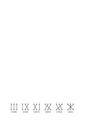
FIG. 1.: Six graphs for the local boundary weight for $S=\frac{3}{2}$. The upper (lower) three circles denote subspins at $\tau=0$ ($\beta$). In general, $(2S)!$ graphs can be labeled uniquely in terms of corresponding permutations of $2S$ integers as shown in the bottom row.

Next, for each local boundary weight $P_{i}(\partial{\cal C}_{i})$, we introduce $(2S)!$ types of graphs $\{{\cal G}_{Pi}\}$ ($i=1,\cdots,N_{\rm s}$), each of which consists of $2S$ edges connecting one of subspins at $\tau=0$ to a subspin at $\tau=\beta$ one by one (Fig. 1). We define a compatibility function $\Delta_{P}(\partial{\cal C}_{i},{\cal G}_{Pi})$ as it takes 1 if every edge connects two subspins which have an identical direction, or it takes 0 otherwise. By using this compatibility function, we can decompose the local boundary weight as

$$P_{i}(\partial{\cal C}_{i})=\sum_{{\cal G}_{Pi}}\Delta_{P}(\partial{\cal C}_{i},{\cal G}_{Pi})/(2S)!\,,$$ (10)

because the number of compatible graphs for a configuration $\partial{\cal C}_{i}$ is given by $(2S-n_{i})!n_{i}!$. We take the labeling probability for the local boundary weight as

$$T_{P}({\cal G}_{Pi}|\partial{\cal C}_{i})=\frac{\Delta_{P}(\partial{\cal C}_{i},{\cal G}_{Pi})/(2S)!}{P_{i}(\partial{\cal C}_{i})}=\frac{\Delta_{P}(\partial{\cal C}_{i},{\cal G}_{Pi})}{(2S-n_{i})!n_{i}!}\,,$$ (11)

that is, a graph is assigned out of the graphs compatible with $\partial{\cal C}_{i}$ with equal probability. These boundary graphs make the remaining opened loops to be closed. By choosing the flipping probability to be free, that is, flipping spins on each loop simultaneously with probability $\frac{1}{2}$, one can show that the present stochastic process satisfies the detailed-balance condition [11].

The present algorithm includes the loop algorithm for the $S=1$ antiferromagnetic Heisenberg model by Harada et al [10] as a special case. However, as already seen, the present strategy does not depend so much on details of the model one considers; one can easily construct a cluster algorithm, if the mapped $S=\frac{1}{2}$ model has a cluster algorithm, which covers a model with general XYZ interaction or single-ion anisotropy [12], and the transverse-field Ising model [13]. It can be applied also for a system with random size of spins and even for the classical Ising model [14, 15]. The resulting general-$S$ algorithm is ergodic, if the $S=\frac{1}{2}$ cluster algorithm lying at the base is ergodic. The details of the algorithm for these models and the proof of its ergodicity will be presented elsewhere [12]. Note that the number of graphs introduced for the local boundary weight increases quite rapidly as $S$ increases. However, the computational time in selecting a graph to be assigned is merely proportional to $S$, because the procedure is nothing but the random-permutation generation[16].

As an application of the algorithm, we simulated the antiferromagnetic Heisenberg chains with $S=1$, 2, and 3. It is conjectured by Haldane [17] that the antiferromagnetic Heisenberg chain of integer spins has a finite excitation gap $\Delta(S)$ above its unique ground state, and the antiferromagnetic spin correlation along the chain decays exponentially with a finite correlation length $\xi_{x}(S)$. For $S=1$ and 2, a number of numerical studies have been accomplished (e.g., see [18, 19, 20, 21]) to confirm the validity of Haldane’s conjecture. However, estimation of the first excitation gap of higher-spin chains has not yet been successful, since the magnitude of $\Delta(S)$ is considered to become exponentially small as $S$ increases [17].

Consider a spin-$S$ chain of $L$ sites at temperature $T$ ($=1/\beta$). We assume $L$ is even. The correlation function of the staggered magnetization in the imaginary-time direction:

$$C(\tau;L,\beta)=\frac{1}{L^{2}\beta}\sum_{i,j=1}^{L}\int_{0}^{\beta}\!dt\,\langle(-1)^{|i-j|}S_{i}^{z}(t)S_{j}^{z}(t+\tau)\rangle$$ (12)

is an even function of $\tau$, and satisfies $C(\tau+\beta;L,\beta)=C(\tau;L,\beta)$. At sufficiently low temperatures, the correlation function is expressed well as a sum of exponential functions, that is,

$$C(\tau;L,\beta)=\sum_{i=0}c_{i}\cosh\left[\frac{\tau-\beta/2}{\xi_{\tau,i}(L)}\right]\ \ \ \mbox{for $\beta\gg\xi_{\tau,0}$.}$$ (13)

Here, we assume $\xi_{\tau,0}>\xi_{\tau,1}>\xi_{\tau,2}>\cdots$ without loss of generality. The coefficients $\left\{c_{i}\right\}$ are directly related to the dynamic structure factor at momentum $k=\pi$. In terms of $\xi_{\tau,0}(L)$, the gap to be estimated is given by

$$\Delta=\lim_{L\rightarrow\infty}\frac{1}{\xi_{\tau,0}(L)}\ .$$ (14)

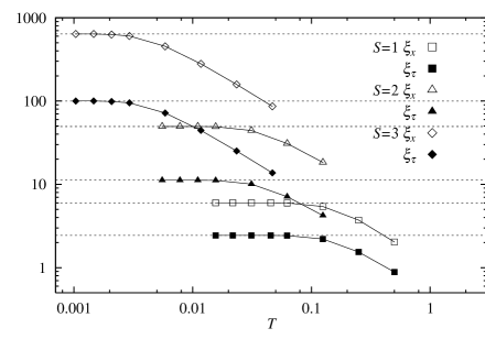
FIG. 2.: Temperature dependence of the spatial correlation length $\xi_{x}$ (open symbols) and the temporal correlation length $\xi_{\tau}$ (solid symbols) of the $S=1$ (squares), 2 (triangles), and 3 (diamonds) antiferromagnetic Heisenberg chains. Statistical error of each data point is smaller than the line width. The system size is taken as $L=2S/T$.

TABLE I.: Ground-state energy density $E/L$, staggered susceptibility $\chi_{\rm s}$, spatial correlation length $\xi_{x}$, and first excited gap $\Delta$ of the $S=1$, 2, and 3 antiferromagnetic Heisenberg chains. Note that for each $S$, the physical quantities are estimated by a single Monte Carlo run on the system of size $L$ at temperature $T$, which are presented in the second and third columns, respectively.

$S$	$L$	$T$	MCS	$E/L$	$\chi_{\rm s}$	$\xi_{x}$	$\Delta$
1	128	0.0156250	$2\times 10^{7}$	-1.401481(4)	18.4048(7)	6.0153(3)	0.41048(6)
2	724	0.0055249	$2\times 10^{6}$	-4.761249(6)	1164.0(2)	49.49(1)	0.08917(4)
3	5792	0.0010359	$3\times 10^{4}$	-10.1239(1)	158000(310)	637(1)	0.01002(3)

In general, to solve Eq. (13) directly is extremely ill-posed [22]. However, as shown below, we can construct a systematic series of estimators at least for $\xi_{\tau,0}(\tau)$, if the coefficient $c_{i}$ in Eq. (13) converges to zero rapidly enough for large $i$, and also if the difference between $\xi_{\tau,0}(L)$ and $\xi_{\tau,1}(L)$ remains finite even in the thermodynamic limit. For S=1, these two conditions are numerically shown to be satisfied [23]. We expect similar situations for higher $S$, although there is no exact argument.

For a given $L$, the well-known second-moment estimator [24] of the correlation length,

$$\hat{\xi}_{\tau}^{(2)}=\frac{\beta}{2\pi}\sqrt{\frac{{\tilde{C}}(0)}{\tilde{C}(2\pi/\beta)}-1},$$ (15)

converges to $\xi_{\tau,0}(L)$ in the low-temperature limit, besides systematic corrections of $O(a_{i}\xi_{\tau,i}/\xi_{\tau,0})$ ($i=1,2,\cdots$). Here, ${\tilde{C}}(\omega)$ is the Fourier transform of the imaginary-time spin correlation function, i.e., $\tilde{C}(\omega)=\int_{0}^{\beta}C(\tau)e^{i\omega\tau}d\tau$. In the present algorithm, $\tilde{C}(\omega)$ can be measured directly by means of the improved estimator[25], which reduces the variance of the data greatly. We also consider a fourth-moment estimator:

$$\hat{\xi}_{\tau}^{(4)}=\frac{\beta}{4\pi}\sqrt{3\frac{{\tilde{C}}(0)-{\tilde{C}}(2\pi/\beta)}{{\tilde{C}}(2\pi/\beta)-{\tilde{C}}(4\pi/\beta)}-1}\,,$$ (16)

which has smaller corrections of $O(a_{i}(\xi_{\tau,i}/\xi_{\tau,0})^{3})$. Construction of higher-order estimators is possible in a straightforward way[12].

The temperature dependence of $\hat{\xi}_{\tau}(L,T)$ and also of the correlation length along the chain, $\hat{\xi}_{x}(L,T)$, is shown in Fig. 2. In the present simulation, the system size is taken as $L=2S/T$. The integrated auto-correlation time of $\tilde{C}(0)$ is of order unity and no significant sign of its growth is observed for larger $L$ and $1/T$. Measurement of physical quantities is performed after discarding first $10^{3}$ Monte Carlo steps (MCS) for thermalization. One Monte Carlo step of the $S=3$ chain with $L=5792$ and $T=0.0010359$, which is mapped to the system of 34752 subspins and 208512 bonds prior to the simulation, takes about 16 seconds on 256 nodes of Hitachi SR-2201.

As seen clearly in Fig 2, $\hat{\xi}_{\tau}(L,T)$ and $\hat{\xi}_{x}(L,T)$ converge quite rapidly (probably exponentially) to a finite value for small $T$. We observe that for each $S$ the data which satisfy the conditions, $1/T>6\hat{\xi}_{\tau}$ and $L>6\hat{\xi}_{x}$, exhibit no temperature (and system-size) dependence besides statistical fluctuations. The difference between the second-moment estimate (Eq. (15)) and the fourth-moment one (Eq. (16)) is invisible in the vertical scale of Fig 2. The difference between these two estimates at the lowest temperature is about 0.2% and 0.1% for $S=1$ and $S=2$, respectively. For $S=3$, both coincide within the statistical errors. Furthermore, it is confirmed that there is no significant difference between the fourth-moment estimate and the sixth-moment one even for $S=1$.

Thus, by using the fourth-moment estimator, we conclude

$$\Delta(S)=\left\{\begin{array}[]{ll}0.41048(6)&\mbox{\ for $S=1$}\\ 0.08917(4)&\mbox{\ for $S=2$}\\ 0.01002(3)&\mbox{\ for $S=3$}\end{array}\right.$$ (17)

as the magnitude of the Haldane gap. The results for other physical quantities, such as the energy density and the staggered susceptibility, are presented in Table I. It should be emphasized that the present results are obtained without any extrapolation procedure; they are simply obtained by a single Monte Carlo run on the largest system at the lowest temperature for each $S$.

For $S=1$, the present estimate is completely consistent with $0.41050(2)$ and $0.41049(2)$ obtained by the DMRG calculation [18] and by the exact diagonalization [19], respectively. For $S=2$, on the other hand, the numerical uncertainty in the present estimate is much smaller than in the previous studies (see, e.g., TABLE I in Ref. [21]). Furthermore, our estimate is slightly larger than $0.0876(13)$, which is obtained by the most recent DMRG calculation [21]. In the DMRG study, for some technical reasons, open boundary conditions have been used, which is known to give quite large systematic corrections compared to the periodic boundary conditions. The reason of the disagreement might be due to an inappropriate scaling assumption in the DMRG study. Finally, as for the $S=3$ case, it might be practically impossible to estimate the value of the gap by other numerical methods. The present result is completely new to our best knowledge.

The present authors would like to thank H. Takayama, N. Kawashima, H. G. Evertz, and K. Hukushima for stimulating discussions and comments. Most of numerical calculations for the present work have been performed on the CP-PACS at University of Tsukuba, Hitachi SR-2201 at Supercomputer Center, University of Tokyo, and the RANDOM at MDCL, Institute for Solid State Physics, University of Tokyo. The present work is supported by the “Large-scale Numerical Simulation Program” of Center for Computational Physics, University of Tsukuba, and also by the “Research for the Future Program” (JSPS-RFTF97P01103) of Japan Society for the Promotion of Science.

REFERENCES

- [1] Present address: Theoretische Physik, Eidgenössische Technische Hochschule, CH-8093 Zürich, Switzerland.
- [2] Present address: Semiconductor Energy Laboratory Co., Ltd., Yokohama 243-0036, Japan.
- [3] For reviews, see e.g., Quantum Monte Carlo Methods in Condensed Matter Physics, ed. M. Suzuki (World Scientific, Singapore, 1994).
- [4] H. G. Evertz, G. Lana, and M. Marcu, Phys. Rev. Lett. 70, 875 (1993).
- [5] U.-J. Wiese and H.-P. Ying, Z. Phys. B 93, 147 (1994).
- [6] B. B. Beard and U.-J. Wiese, Phys. Rev. Lett. 77, 5130 (1996).
- [7] H. G. Evertz, unpublished (cond-mat/9707221), and references therein.
- [8] N. Kawashima and J. E. Gubernatis, Phys. Rev. Lett. 73, 1295 (1994); J. Stat. Phys. 80, 169 (1995).
- [9] Y. J. Kim, M. Greven, U.-J. Wiese, and R. J. Birgeneau, Eur. Phys. J. B 4, 291 (1998).
- [10] K. Harada, M. Troyer, and N. Kawashima, J. Phys. Soc. Jpn. 67, 1130 (1998).
- [11] N. Kawashima and J. E. Gubernatis, Phys. Rev. E 51, 1547 (1995).
- [12] S. Todo and K. Kato, unpublished.
- [13] H. Rieger and N. Kawashima, Europ. Phys. J. B 9, 233 (1999).
- [14] R. H. Swendsen and J. S. Wang, Phys. Rev. Lett. 58, 86 (1987).
- [15] S. Todo and K. Kato, Prog. Theor. Phys. Suppl. 138, 535 (2000).
- [16] D. E. Knuth, The Art of Computer Programing, Seminumerical Algorithms, 3rd ed. (Addison Wesley, Reading, 1998) p. 145.
- [17] F. D. M. Haldane, Phys. Lett. 93A, 464 (1983); Phys. Rev. Lett. 50, 1153 (1983).
- [18] S. R. White and D. A. Huse, Phys. Rev. B 48, 3844 (1993).
- [19] O. Golinelli, Th. Jolicœur, and R. Lacaze, Phys. Rev. B 50, 3037 (1994).
- [20] U. Schollwöck and Th. Jolicœur, Europhys. Lett. 30, 493 (1995).
- [21] X. Wang, S. Qin, and L. Yu, Phys. Rev. B 60, 14529 (1999).
- [22] R. N. Silver, D. S. Sivia, and J. E. Gubernatis, Phys. Rev. B 41, 2380 (1990).
- [23] M. Takahashi, Phys. Rev. B 50, 3045 (1994).
- [24] F. Cooper, B. Freedman, and D. Preston, Nuc. Phys. B 210 [FS6], 210 (1982).
- [25] G. A. Baker, Jr., and N. Kawashima, Phys. Rev. Lett. 75, 994 (1995).