The Role of Domain Walls on the Vortex Creep Dynamics in Unconventional Superconductors

1 Introduction

The penetration of magnetic fields into type-II superconductors as flux lines (vortices) yields many complex phenomena. In recent years the physics of vortices has become an important subject, particularly in connection with high-temperature superconductivity. [1] The physics of “vortex matter” is crucial for a large number of applications of superconductivity involving high currents and fields. Vortices limit the technological capability of superconductors, since their motion generates dissipation. Therefore one of the central issues is the pinning of vortices at defects such as impurities, lattice dislocations and twin boundaries. The critical current, the limit of dissipation-free transport, depends on the character and strength of the pinning potentials created by these defects. The effect of pinning was shown to crucially depend on the various phases of vortex matter, and the resulting problems are naturally very complex. [1]

In this paper we would like to discuss a pinning phenomenon in unconventional superconductors which has a character different from the usual pinning at crystal defects. This study is motivated by recent experiments on heavy fermion compounds UPt₃ and U_1-xTh_xBe₁₃ as well as on the transition metal oxide Sr₂RuO₄ [2, 3, 4, 5]. All these superconductors have a comparatively low transition temperature of the order of 1K. Fluctuation effects do not play an important role in these systems. However, interesting vortex physics is introduced because the superconducting order parameter of these systems has more than one component. This yields more degrees of freedom in forming topologically stable defects of the order parameter, a well-known feature in superfluid ³He physics. We would first like to review some of the basic experimental facts concerning the mixed state of these three superconductors, which will be relevant for our theoretical discussion.

One aspect of the mixed state related to vortex pinning is the slow motion of vortices close to the critical state, known as flux creep. This phenomenon is observed as the slow decrease of the remnant magnetization after the superconductor has been exposed for some time to a magnetic field considerably larger than the lower critical field, $H_{c1}$. The remnant magnetization that exists after turning off the external field originates from the pinning of vortices in the material. The motion of these vortices out of the sample, generally governed by thermally activated crossing of pinning potential barriers, leads to the slow decay of the magnetization.[1] (Note that quantum phenomena, macroscopic quantum tunneling, can also play an important role at sufficiently low temperature. [1, 6]) The decay (creep) rate is determined by the temperature, the pinning properties, and the vortex matter state as described by Kim and Anderson [7, 8] (see also Geshkenbein and Larkin [9]). A simple and intuitive theory of the critical vortex state in a material with strong pinning effects was given by Bean.[10] It describes the characteristic profile of the vortex distribution depending on the history of the external applied fields and the critical current. [8]

In the two heavy Fermion superconductors UPt₃ and U_0.9725Th_0.0275Be₁₃ ($0.017\leq x\leq 0.45$), an anomalous temperature dependence of the creep rate was observed by Mota’s group. [2, 3] UPt₃ and U_1-xTh_xBe₁₃ ($0.017\leq x\leq 0.45$) both exhibit two consecutive superconducting phase transitions. Flux relaxation measurements show a rapid drop of the creep rate, essentially to zero, immediately below the second transition in both system.[2, 3] A similar sudden drop in the creep rate was reported for Sr₂RuO₄ at the rather low temperature $T^{*}\approx 50$ mK. [4] In contrast to the former two examples, no sign of an additional transition at this temperature is observed in any other properties to this time. The transition in the creep rate indicates the onset of a new efficient pinning mechanism which inhibits the motion of vortices from the interior to the surface of the sample. However, it has been noticed in experiments that after a long waiting period some creep recovers. [2, 4]

This effect is readily explained if we assume that fence-like structures exist which prevent the passage of vortices (so that the vortices cannot leave the sample). Experiments indicate that these fences are activated below a certain transition temperature within the superconducting phase. The effect of the fences is rather different to standard pinning. In particular, their influence on the critical current is weak, as discussed below. This is consistent with hysteresis measurements on UPt₃ in a slowly oscillating magnetic field. [5] While the flux creep disappears in the low-temperature phase, the critical current is continuously increasing and shows no anomaly upon entering the low temperature phase. [2, 3] Furthermore, below the second transition Rosenbaum’s group found that the magnetization curves of the hysteresis cycle display strong variations from cycle to cycle in the region close to $H_{c1}$, while in the high field part of the cycle (connected with the critical current of the superconductor) no unusual behavior is seen [5]. This “noise” can be understood as being induced by the weakly mobile fences inhibiting the free flow of vortices. In every cycle the position of the fences changes slightly, and the magnetization process for small vortex concentrations, i.e. for fields close to $H_{c1}$, is modified. [5] We will show that a simulation with a simple model incorporating this effect gives rise to the features observed in these experiments.

What is the origin of these fence-like structures? In unconventional superconductors such structures occur if the superconducting phase is degenerate, e.g., for time-reversal symmetry breaking states which have at least a two-fold degeneracy. Degenerate states can appear as domains in the superconductor accompanied by domain walls as topological structures of the order parameter. [11] Various properties of such domain walls have been studied by several groups. [11, 12, 13] Domain walls in time-reversal symmetry breaking superconductors possess interesting magnetic properties and carry chiral quasiparticle bound states.[12, 13, 14] The question arises whether or not they serve as barriers to the vortex motion. The domain wall is naturally accompanied by a slight local suppression of the order parameter which tends to trap vortices. In this case the pinning strength is rather weak and should not have much influence on the flux motion. However, strong pinning can arise from properties of the internal structure of domain walls. Under certain circumstances the domain wall has, in addition to a stable structure, metastable structures, or even two degenerate stable states. [11] These states may form domains on the domain wall that are separated by line defects. It has been shown that such lines carry a magnetic flux which is an arbitrary fraction of a standard flux quantum in a superconductor.[13] We will show that an ordinary vortex placed on such a domain wall can decay into two fractional vortices. [13, 15] Since these fractional vortices can only exist on the domain wall, they are strongly pinned. They repel other approaching vortices, and in this way the domain wall indeed acts as a strong barrier. A high density of vortices close to the domain wall can destroy the state which carries fractional vortices, and the pinning effect disappears. This is equivalent to having a barrier “height” for the vortex pinning. It is important to note that this pinning property of the domain wall does not alter the bulk pinning due to impurities within each domain. This type of impurity-based pinning is responsible for determining the critical current. However, the domain walls play an important role in the overall flux motion. They are the origin of an intrinsic pinning location created by the superconducting state itself, in contrast to the extrinsic pinning due to material defects. Note, however, that the domain walls themselves are pinned at lattice defects reducing their mobility.

In this article we first discuss properties of domain walls in the most simple case of a time-reversal symmetry breaking superconducting state using the Ginzburg-Landau theory. Then we use the domain walls as barriers in a model based on the Bean’s theory and consider the modification of flux motion properties due to these barriers.

2 Properties of a domain wall

In this section we investigate the structure of a domain wall in a time-reversal symmetry breaking superconducting state as may be realized in the low-temperature phases of UPt₃ and U_1-xTh_xBe₁₃, and at the onset of superconductivity in Sr₂RuO₄. We do not include the aspects of the double transition related to the former two, as it complicates the discussion considerably without leading to further insight.

2.1 Ginzburg-Landau theory

For the following discussion we introduce the simplest possible model that contains all the relevant features in order to discuss the physics of domain walls in an unconventional superconductor. We consider a system with tetragonal crystal symmetry based on the point group $D_{4h}$. The superconducting order parameter shall belong to the two-dimensional representation $E_{g}$ (even parity) or $E_{u}$ (odd parity), yielding the following expansion for the gap functions ($2\times 2$ gap matrix with the notation $\hat{\mathchar 28929\relax}=i\hat{\sigma}_{y}\psi$ for even and $\hat{\mathchar 28929\relax}=i(\mbox{\boldmath$d$}\cdot\hat{\mbox{\boldmath$\sigma$}})\hat{\sigma}_{y}$ for odd parity):

$$\begin{array}[]{l}\psi(\mbox{\boldmath$k$})=(\eta_{x}v_{z}v_{x}+\eta_{y}v_{z}v_{y})/\langle v_{x}^{2}v_{z}^{2}\rangle,\\ \\ \mbox{\boldmath$d$}(\mbox{\boldmath$k$})=\hat{{\bf z}}(\eta_{x}v_{x}+\eta_{y}v_{y})/\langle v_{x}^{2}\rangle.\\ \end{array}$$ (2.1)

Here $\mbox{\boldmath$\eta$}=(\eta_{x},\eta_{y})$ represent the two-dimensional complex order parameter, $\hat{{\bf z}}$ denotes the unit vector along $z$-direction, $v_{i}$ denotes the components of the Fermi velocity, and $\langle...\rangle$ is the average over the Fermi surface. As mentioned above, we concentrate on the time-reversal symmetry breaking states of the form $\mbox{\boldmath$\eta$}\propto(1,\pm i)$ yielding the gap functions

$$\psi(\mbox{\boldmath$k$})=\eta_{0}v_{z}(v_{x}\pm iv_{y})/\langle v_{x}^{2}v_{z}^{2}\rangle\qquad{\rm or}\qquad\mbox{\boldmath$d$}(\mbox{\boldmath$k$})=\hat{{\bf z}}(v_{x}\pm iv_{y})/\langle v_{x}^{2}\rangle.$$ (2.2)

It is convenient to transform the order parameter into the basis set $\eta_{\pm}=(\eta_{x}\mp i\eta_{y})/\sqrt{2}$. For simplicity we also use the phenomenological parameters as determined by weak coupling theory and assume that $v_{z}$ does not depend upon $k_{x}$ or $k_{y}$. The general GL free energy then has the form

$$\begin{array}[]{ll}\displaystyle{\cal F}=\int d^{3}r&[\displaystyle a(|\eta_{+}|^{2}+|\eta_{-}|^{2})+b\{(|\eta_{+}|^{4}+|\eta_{-}|^{4})+4|\eta_{+}|^{2}|\eta_{-}|^{2}\\ &\\ &\displaystyle+\nu(\eta_{-}^{*2}\eta_{+}^{2}+\eta_{-}^{2}\eta_{+}^{*2})\}+\kappa\{|\mbox{\boldmath$D$}\eta_{+}|^{2}+|\mbox{\boldmath$D$}\eta_{-}|^{2}\\ &\\ &\displaystyle+\frac{1}{2}((D_{-}\eta_{+})^{*}(D_{+}\eta_{-})+\nu(D_{+}\eta_{+})^{*}(D_{-}\eta_{-})+{\rm c.c.})\}+\frac{1}{8\pi}(\nabla\times\mbox{\boldmath$A$})^{2}].\\ &\end{array}$$ (2.3)

Here $a=a_{0}(T-T_{c})$ and $b$ and $\kappa$ are the standard coefficients derived from the weak coupling theory. In the gradient terms, we use the gauge invariant derivatives $\mbox{\boldmath$D$}=\mbox{\boldmath$\nabla$}-i\gamma\mbox{\boldmath$A$}$, with $D_{\pm}=D_{x}\pm iD_{y}$ and $\gamma=2e/\hbar c=2\pi/\mathchar 28936\relax_{0}$ ($\mathchar 28936\relax_{0}$ is the flux quantum). The parameter $\nu$ denotes the deviation of the Fermi surface or its density of states from cylindrical symmetry around the $z$-axis due to the tetragonal crystal field

$$\nu=\frac{\langle v_{x}^{4}\rangle-3\langle v_{x}^{2}v_{y}^{2}\rangle}{\langle v_{x}^{4}\rangle+\langle v_{x}^{2}v_{y}^{2}\rangle},$$ (2.4)

where $\nu=0$ for a cylindrical symmetric Fermi surface. In this form the GL theory describes two degenerate superconducting states, $(\eta_{+},\eta_{-})=\eta_{0}(T)(1,0)$ and $\eta_{0}(T)(0,1)$ with

$$\eta_{0}^{2}(T)=\frac{a_{0}(T_{c}-T)}{2b}.$$ (2.5)

for $T<T_{c}$.

In the following we analyze the properties of domain walls between the two degenerate states. We assume that they are infinite and planar such that we can separate the coordinates into components parallel and perpendicular to the normal vector $n$ of the domain wall. For simplicity we ignore the $z$-direction, assuming that $\mbox{\boldmath$n$}\perp{\bf z}$. Therefore it is convenient to rewrite the free energy in these coordinates: $(x,y)\to(x^{\prime},y^{\prime})=(r_{\parallel},r_{\perp})$ and $D_{\pm}=e^{\pm i\theta}D^{\prime}_{\pm}$. Simultaneously we transform the order parameter $\eta_{\pm}=e^{\pm i\theta}\eta^{\prime}_{\pm}$ so that the gradient terms become

$$\kappa\{|\mbox{\boldmath$D$}^{\prime}\eta^{\prime}_{+}|^{2}+|\mbox{\boldmath$D$}^{\prime}\eta^{\prime}_{-}|^{2}+\frac{1}{2}((D^{\prime}_{-}\eta^{\prime}_{+})^{*}(D^{\prime}_{+}\eta^{\prime}_{-})+\nu e^{-i4\theta}(D^{\prime}_{+}\eta^{\prime}_{+})^{*}(D^{\prime}_{-}\eta^{\prime}_{-})+c.c.)\}$$ (2.6)

and in the homogeneous part only the third term among the fourth order terms is modified to

$$b\nu e^{i4\theta}\eta_{-}^{\prime*2}\eta_{+}^{\prime 2}+{\it c.c.}$$ (2.7)

From this point we omit the primes for coordinates and order parameters and take $\theta$ as the angle of the normal vector $n$ relative to the crystal $x$-axis. Thus, the $x(y)$-coordinate is now always parallel (perpendicular) to the normal vector. In this representation the $\theta$ dependence clearly does not appear, if the system is cylindrically symmetric, i.e., $\nu=0$.

2.2 Structure of the domain wall

We now turn to the domain wall and consider the situation in which for $x\to\pm\infty$ the superconducting states $\eta_{\pm}$ is realized and around $x=0$ a smooth change between

Fig. 1: Schematic behavior of the order parameter components at the domain wall.

the two states occurs within a finite length scale (Fig. 1). This situation is similar to a Josephson junction between two superconductors with the state $\eta_{+}$ and $\eta_{-}$, respectively. Indeed the phase difference between the two states plays a similarly important role for the physical properties of the domain wall. The structure of the domain wall is obtained by a variational minimization of the free energy ${\cal F}$. For the sake of transparency we simplify the treatment by introducing the following approximate variational ansatz for the order parameter:

$$\eta_{+}=\eta_{0}e^{i\phi_{+}}\cos\chi\qquad{\rm and}\qquad\eta_{-}=\eta_{0}e^{i\phi_{-}}\sin\chi.$$ (2.8)

This leads to the boundary conditions

$$\chi=\left\{\begin{array}[]{ll}0&\qquad x\to+\infty,\\ &\\ \displaystyle\frac{\pi}{2}&\qquad x\to-\infty\end{array}.\right.$$ (2.9)

We assume spatial dependence only for $\chi$ and leave the phase difference between the two sides $\alpha=\phi_{+}-\phi_{-}$ constant. The effective free energy becomes

$$\begin{array}[]{ll}\tilde{\cal F}=\int d^{3}r&[\displaystyle a\eta_{0}^{2}+b\eta_{0}^{4}+\frac{b\eta_{0}^{4}}{2}(1+\nu\cos(2\alpha+4\theta))\sin^{2}2\chi\\ &\\ &\displaystyle+\kappa\eta_{0}^{2}\{|\mbox{\boldmath$D$}\cos\chi|^{2}+|\mbox{\boldmath$D$}\sin\chi|^{2}+[e^{-i\alpha}(D_{-}\cos\chi)^{*}(D_{+}\sin\chi)\\ &\\ &\displaystyle+\nu e^{-i(\alpha+4\theta)}(D_{+}\cos\chi)^{*}(D_{-}\sin\chi)+c.c]/2\}+\frac{1}{8\pi}(\nabla\times\mbox{\boldmath$A$})^{2}].\\ &\end{array}$$ (2.10)

We neglect contributions from $A_{y}$ and vary the free energy with respect to $\chi$,

$$\partial_{x}^{2}\chi=\frac{Q}{4}\sin 4\chi-4S_{+}\gamma A_{x}(\partial_{x}\chi)+2C_{+}(\sin 2\chi\partial_{x}^{2}\chi+\cos 2\chi[(\partial_{x}\chi)^{2}+\gamma^{2}A_{x}^{2}]),$$ (2.11)

and $A_{x}$,

$$A_{x}=\frac{S_{+}\partial_{x}\chi}{\gamma(1+C_{+}\sin 2\chi)},$$ (2.12)

with

$$Q =\frac{1}{\xi_{0}^{2}}\{1+\nu\cos(2\alpha+4\theta)\},$$ (2.13)

$$C_{\pm} =\left[\cos\alpha\pm\nu\cos(\alpha+4\theta)\right]/2,$$

$$S_{\pm} =\left[\sin\alpha\pm\nu\sin(\alpha+2\theta)\right]/2,$$

and $\xi_{0}^{2}=\kappa/2b\eta_{0}^{2}$. The third term on the right-hand side of Eq. (2.11) and the $\sin{2\chi}$ term in the denominator of $A_{x}$ complicate the solution. We find, however, that the influence of these terms is small at larger distances from the domain wall, as one can see in approximating $\chi(x)\approx e^{-Kx}$ in the limit $x\to+\infty$. With this ansatz, Eq. (2.11) becomes

$$(1-S_{+}^{2})K^{2}e^{-Kx}=Qe^{-Kx}+O(e^{-2Kx}).$$ (2.14)

Thus the second term decays much faster than the first one. Therefore, the width of the domain wall is largely determined by the first term, and the second term enters only into the domain wall energy.

Fig. 2: The domain wall energies as functions of the phase difference $\alpha=\phi_{+}-\phi_{-}$ for angles $\theta=0,\pi/8$ and $\pi/4$. The anisotropy parameter is chosen $\nu=-0.5$.

We solve Eq. (2.11) neglecting the third term and the $\sin{2\chi}$ term in the denominator of $A_{x}$, so that it takes the form of an ordinary Sine-Gordon equation,

$$\partial_{x}^{2}\chi=\frac{\tilde{Q}}{4}\sin 4\chi,$$ (2.15)

where $\tilde{Q}=Q/(1-S_{+}^{2})$ for which we easily find the kink solution

$$\chi(x)={\rm arctan}(e^{-x\sqrt{\tilde{Q}}}).$$ (2.16)

This is used to determine $A_{x}$ through Eq. (2.12) and both $A_{x}$ and $\chi$ are inserted into the free energy and integrated, so that we obtain for the variational domain wall energy

$$f(\alpha,\theta)=\kappa\eta_{0}^{2}\sqrt{\tilde{Q}}\left\{1-\frac{C_{+}\pi}{8}-\frac{S_{+}^{2}}{C_{+}}\left[\frac{\pi}{4}-\frac{1}{\sqrt{1-C_{+}^{2}}}{\rm arctan}\left(\frac{\sqrt{1-C_{+}^{2}}}{1+C_{+}}\right)\right]\right\}$$ (2.17)

as a function of $\alpha$ and $\theta$.

From this point we fix $\nu<0$. For sufficiently large $|\nu|$ the domain wall energy develops two local minima as a function of the relative phase $\alpha$. This is illustrated in Fig. 2 for angles $\theta=0,\pi/8$ and $\pi/4$. For the most stable orientation $\theta=0$ these minima are at $\alpha=0$ (stable state) and $\alpha=\pi$ (metastable state). For $\theta\to\pi/4$ we find that the stable and metastable state approach in energy and become degenerate at exactly $\theta=\pi/4$. The presence of stable and metastable states is important when we discuss vortex states on the domain wall.

3 Vortices on the domain wall

We now investigate local modifications of the domain wall structure which give rise to vortices. This problem has been previously considered for the case of the degenerate domain wall state. [13] Here we extend the discussion to the general situation.

3.1 Fractional flux lines

As mentioned in the Introduction, domain walls act as pinning regions for the vortices (core pinning) due to the locally diminished condensation energy. The resulting pinning effect is, however, rather small, since the domain wall only provides a shallow attractive potential. In the following we would like to show that a change of the vortex structure can lead to considerable strengthening of the pinning potential.

To some extent the domain wall can be viewed as a planar weak link between two superconductors with order parameters slightly interpenetrating, as described by Eq. (2.8). We use this form for the order parameter to express the current which is obtained from the variation of the free energy with respect to the vector potential,

$$\begin{array}[]{l}\displaystyle j_{x}=\frac{\kappa\gamma}{c}[2\cos^{2}\chi u_{x+}+2\sin^{2}\chi u_{x-}-\sin 2\chi\{(u_{x+}+u_{x-})C_{+}+(u_{y+}+u_{y-})S_{-}\}+2(\partial_{x})\chi S_{+}],\\ \\ \displaystyle j_{y}=\frac{\kappa\gamma}{c}[2\cos^{2}\chi u_{y+}+2\sin^{2}\chi u_{y-}-\sin 2\chi\{(u_{y+}+u_{y-})C_{+}+(u_{x+}+u_{x-})S_{-}\}+2(\partial_{x})\chi C_{-}],\\ \end{array}$$ (3.1)

with

$$u_{\mu\pm}=\eta^{2}_{0}(\partial_{\mu}\phi_{\pm}-\gamma A_{\mu}).$$ (3.2)

In the stable and metastable states for given $\theta$, the current perpendicular to the domain wall should vanish. If this were not the case, current would flow everywhere in the bulk, leading to a large energy cost. Neglecting the contributions of $A_{y}$ leads to Eq. (2.12) for $A_{x}$, so that the variational solution already ensures that the current perpendicular to the wall vanishes for $\alpha$ of the (meta)stable state.

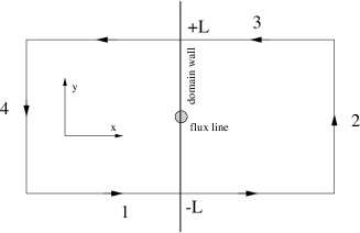
Fig. 3: Rectangular path encircling the flux line. We separate the path into parts 1, 2, 3 and 4 in order to calculation the contribution to the flux.

We now consider vortices on the domain wall corresponding to the winding of the order parameter phase. By analogy to Josephson junctions, such a vortex may be considered a “kink” of the phase difference $\alpha$. In the ordinary case, the size of the kink is an integer multiple of $2\pi$. For the domain wall it is, however, possible to generate a kink to a metastable state. While, in general, a $2\pi$-kink is associated with the standard magnetic flux quantum $\mathchar 28936\relax_{0}=hc/2e$, a smaller kink between the stable and metastable state would carry a fraction of $\mathchar 28936\relax_{0}$ only, depending on the size of the kink and other parameters. For the Josephson junction we can describe the vortex using a Sine-Gordon equation of the phase difference containing only one length scale, the Josephson penetration depth. This analogy, however, is limited, because in the case of the domain wall two length scales have to be taken into account: the coherence length $\tilde{\xi}$ (length scale of the variation of $\alpha$) along the domain wall and the London penetration depth $\lambda_{L}$. We consider the limit $\lambda_{L}\gg\tilde{\xi}$, ignore the detailed structure of the vortex on small length scales ($\sim\tilde{\xi}$) and focus mainly on its magnetic properties.

Let us analyze now a kink of $\alpha$ as a line defect in the domain wall between the stable state with $\alpha=\alpha_{0}$ and the metastable state with $\alpha=\alpha_{1}$. We encircle this line by a wide rectangular path (see Fig. 3) and calculate the enclosed magnetic flux $\mathchar 28936\relax=\oint d{\bf s}\cdot\mbox{\boldmath$A$}$. First, we consider the parts of the path which cross the domain wall perpendicularly, 1 and 3. We choose the gauge such that $\partial_{x}\phi_{\pm}=0$ along both paths, i.e., any variation of $\phi_{\pm}$ is restricted to the parts of the path parallel to the domain wall. If we now use the condition $j_{x}=0$ along this path, we obtain the contribution

$$\varphi_{1}=\int^{+\infty}_{-\infty}dxA_{x}(x,y=-L)=\int^{\pi}_{0}d\beta\frac{S_{+}}{2\gamma}\frac{1}{1+C_{+}\sin\beta}=\mathchar 28936\relax_{0}\mathchar 28933\relax(\alpha_{0},\theta)$$ (3.3)

to the flux from path 1, where

$$\mathchar 28933\relax(\alpha,\theta)=\frac{S_{+}}{2\pi\sqrt{1-C^{2}_{+}}}\left[{\rm arctan}\left(\frac{C_{+}}{\sqrt{1-C^{2}_{+}}}\right)-\frac{\pi}{2}\right].$$ (3.4)

Analogously, the contribution from path 3 is given by

$$\varphi_{3}=\int^{-\infty}_{+\infty}dxA_{x}(x,y=+L)=-\mathchar 28936\relax_{0}\mathchar 28933\relax(\alpha_{1},\theta),$$ (3.5)

and for the paths 2 and 4 we take the variation of $\phi_{\pm}$ into account. With $j_{y}=0$ sufficiently far from the domain wall, this leads to

$$\begin{array}[]{ll}\varphi_{2}+\varphi_{4}&=\displaystyle\int^{+L}_{-L}dy(A_{y}(x\to+\infty,y)-A_{y}(x\to-\infty,y))\\ &\\ &\displaystyle=\frac{1}{\gamma}\int^{+L}_{-L}(\partial_{y}\phi_{+}\partial_{y}\phi_{-})=\frac{\alpha_{1}-\alpha_{0}+2\pi n}{2\pi}\mathchar 28936\relax_{0}\\ &\end{array}$$ (3.6)

Thus, the flux for the line defect depends on the angle $\theta$ as

$$\mathchar 28936\relax(\theta)=\mathchar 28936\relax_{0}\left[\frac{\alpha_{1}-\alpha_{0}}{2\pi}+\mathchar 28933\relax(\alpha_{0},\theta)-\mathchar 28933\relax(\alpha_{1},\theta)\right]+\mathchar 28936\relax_{0}n,$$ (3.7)

which determines the flux up to an integer multiple of $\mathchar 28936\relax_{0}$. The possible magnetic fluxes are fractional and the smallest ones are smaller than $\mathchar 28936\relax_{0}$ in magnitude. This is analogue to the Josephson vortices on a time-reversal symmetry breaking Josephson junction.[16, 17, 18, 19] In that case, however, the two junction states separated by the flux line are degenerate. This is the case here only for the special angles $\theta=\pm\pi/4$. In the special case $\theta=0$ the phase differences $\alpha_{0}=0$ and $\alpha_{1}=\pi$ lead to $\mathchar 28936\relax=\pm\mathchar 28936\relax_{0}/2$, half a flux quantum. In all other cases the flux depends continuously on $\theta$ and $\nu$.

It is easy to see that two kinks in sequence (stable $\to$ metastable $\to$ stable) yield a total flux $\mathchar 28936\relax=\mathchar 28936\relax_{0}n$. Therefore, a conventional vortex (flux $\mathchar 28936\relax_{0}$) may decay into two fractional vortices on the domain wall (Fig. 4). Through this dissociation, the magnetic field energy can be reduced. If we assume that the domain wall is in the stable state, then the splitting of the vortex introduces a metastable domain wall connecting the two fractional flux lines. Thus, the cost of domain wall energy has to be compensated by the reduction of magnetic energy.

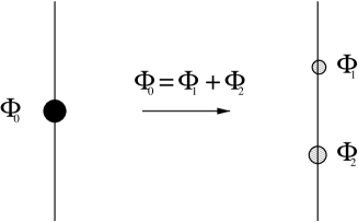
Fig. 4: A standard vortex with flux $\mathchar 28936\relax_{0}$ on the domain wall decays into two fractional vortices whose fluxes add up to $\mathchar 28936\relax_{0}$.

Let us compare the two energies here. The domain wall energy cost per unit area is $\epsilon_{dw}=f_{dw}(\alpha_{1},\theta)-f_{dw}(\alpha_{0},\theta)$, with $f_{dw}$ defined in Eq. (2.17). The magnetic energy of the flux lines can be estimated by assuming that their field distribution is not much different from that of a standard vortex described by the London equation with the free energy functional

$$F_{L}=\int d^{3}r[{\bf B}^{2}+\lambda_{L}^{2}(\nabla\times{\bf B})^{2}],$$ (3.8)

where we assume that the London penetration depth is not modified by the domain wall. We now consider two fractional fluxes, $\mathchar 28936\relax_{1},\mathchar 28936\relax_{2}>0$, with $\mathchar 28936\relax_{1}+\mathchar 28936\relax_{2}=\mathchar 28936\relax_{0}$ (field along the $z$-axis) at the positions ${\bf r}_{1}$ and ${\bf r}_{2}$, respectively. The resulting London equation is

$$B_{z}-\lambda_{L}^{2}\nabla^{2}B_{z}=\mathchar 28936\relax_{1}\delta^{(2)}({\bf r}-{\bf r}_{1})+\mathchar 28936\relax_{2}\delta^{(2)}({\bf r}-{\bf r}_{2}),$$ (3.9)

which is taken in two dimensions, assuming homogeneity along the $z$-axis (${\bf r}=(x,y)$). The solution of the equation leads to the line energies $\varepsilon_{1}$ and $\varepsilon_{2}$ for the two vortices and an interaction energy that depends on the distance between the vortices. Thus the total magnetic energy is

$$v(|y_{2}-y_{1}|)=\varepsilon_{1}+\varepsilon_{2}+\frac{2\mathchar 28936\relax_{1}\mathchar 28936\relax_{2}}{(4\pi\lambda_{L})^{2}}K_{0}\left(\frac{|y_{2}-y_{1}|}{\lambda_{L}}\right),$$ (3.10)

with $K_{0}$ denoting the MacDonalds function. The line energies contain as a lower cutoff length $\tilde{\xi}_{j}$ ($j=1,2$), which is of a magnitude similar to the coherence length,

$$\varepsilon_{j}=\frac{\mathchar 28936\relax_{j}^{2}}{4\pi\lambda_{L})^{2}}{\rm ln}\left(\frac{\lambda_{L}}{\tilde{\xi}_{j}}\right).$$ (3.11)

The potential for the fractional vortex at a distance $R=|y_{2}-y_{1}|$ is therefore

$$V(R)=v(R)+\epsilon_{dw}R-\varepsilon_{0},$$ (3.12)

where $\varepsilon_{0}$ is the line energy per unit length of a standard vortex. The energy loss due to the metastable state introduces a string potential between the two vortices. The optimal distance $R$ is chosen to minimize the potential energy $V(R)$, which corresponds to a pinning potential for the vortex. Note that this potential is only valid for $R\gg\tilde{\xi}_{j}$. Decaying into two fractional vortices leads to a very effective pinning, since the recombination is necessary in order to dislocate the vortex again from the domain wall. This occurs if the two fractional vortices are forced to approach to $R\sim\tilde{\xi}_{j}$.

For a comparison of the energies involved, we estimate the magnetic energy gained by the decay into fractional vortices,

$$\frac{\mathchar 28936\relax_{0}^{2}}{(4\pi\lambda_{L})^{2}},$$ (3.13)

where the London penetration depth is $\lambda_{L}^{2}=1/8\pi\kappa\eta_{0}^{2}\gamma^{2}$. The maximal string energy is obtained for $\theta=0$, where

$$\epsilon_{dw}R\sim\frac{\mathchar 28936\relax_{0}^{2}}{(4\pi\lambda_{L})^{2}}\frac{\kappa}{8}(1+\nu)^{3/2}\frac{R}{\lambda_{L}}.$$ (3.14)

In this case the two energies become comparable for $R$ just a fraction of $\lambda_{L}$. For angles $\theta$ closer to $\pm\pi/4$, the string potential is smaller and the optimal separation is larger. Furthermore, we find that increasing the anisotropy of the Fermi surface, denoted by $\nu$, tends to stabilize fractional vortices. The stability of the fractional vortices does also depend on temperature, because the internal structure of the domain wall can change with lowering temperature. [20]

In this discussion we have assumed that the domain wall is an infinite plane with one fixed $\theta$. In real materials this is not the case, because domain walls are pinned at impurities and lattices defects and, consequently, may change orientation by having “corners”. Since the phase value $\alpha$ for the stable domain wall structure depends on $\theta$, a kink of $\alpha$ should occur at every such corner and, according to our analysis, be accompanied by a flux line. Similarly, one can see that the crossing of two domain walls introduces a fractional vortex along the cutting line. In general, the phase and flux structure of a non-planar domain wall can be rather complicated. However, we do not consider these aspects any further here.

3.2 Barrier effect of a domain wall

We now turn to the situation in which the superconductor is in the mixed phase and contains many vortices. If the conditions are appropriate, some of the vortices will be trapped by the domain wall and decay into fractional vortices. These flux lines are strongly pinned and may form a queue on the domain wall like the planks of a fence. Other vortices approaching the domain wall now are repelled by this vortex fence and cannot easily penetrate or traverse the domain wall (Fig. 5). In this way the domain wall acts as a very effective barrier for vortices.

The question arises under which conditions the domain wall becomes permeable again. The vortices outside the domain wall generate a pressure on the fractional vortices, influencing their density and, hence, their mutual distance. With increasing external vortex density $\rho=B/\mathchar 28936\relax_{0}$ the distance $R$ should shrink. This may be described qualitatively by adding a term $a_{\rm ext}R^{2}$ to the potential $V(R)$ where $a_{\rm ext}>0$ grows with increasing $\rho$ at the domain wall. Hence, it is clear that a growing density of vortices close to the domain wall forces eventually the fractional vortices to recombine when $R\sim\tilde{\xi}$, the extension of the kinks of $\alpha$. The recombined vortices are only weakly pinned so that the fence becomes permeable. This process needs not occur over all the domain wall simultaneously , but may start with local leaks for vortices to pass through. A simple picture of the “barrier height” of the domain wall can be obtained by the following argument. The density of fractional vortices is more or less equal to that of the vortices immediately outside of the domain wall. Therefore, the relation for the spacing $R\sim\rho^{-1/2}=(\mathchar 28936\relax_{0}/B)^{-1/2}$ leads to the barrier field $B^{*}\propto\tilde{\xi}^{-2}$. The temperature dependence of $\tilde{\xi}$ close to the transition temperature (the second transition in the case of a system with double transition) is essentially proportional to $|T-T_{c}|^{-1/2}$ so that the barrier field is growing as the temperature is lowered $B^{*}\propto|T-T_{c}|$.

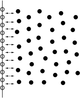
Fig. 5: Schematic picture of a domain wall occupied by fractional flux line (shaded) which repel approaching vortices (filled circles) so that they do not traverse the domain wall.

With these properties, the presence of domain walls should have considerable influence on the flux motion in the lower range of magnetic fields in the mixed phase. In particular this is true for phenomena like flux creep and hysteresis behavior of the mixed phase. We first discuss the influence of the barrier effect on the flux creep which can be observed in the relaxation of remnant magnetization after a magnetic field has been applied for some time to a superconductor and then switched off. The flux relaxation behavior has been investigated in much detail by the group of Mota for the heavy Fermion superconductors UPt₃ and U_1-xTh_xBe₁₃ and for Sr₂RuO₄. [2, 3, 4] The first two superconductors exhibit double transitions, where the low-temperature phase in each case is very likely time-reversal symmetry breaking and should therefore provide the conditions for domain walls as described above. Mota and coworkers observed that the initial flux relaxation rate drops drastically below the second superconducting transition. Hence, many vortices generating the remnant magnetization find it apparently more difficult to escape from the sample in the low-temperature phase. While initially almost no remnant flux leaves, the relaxation recovers after a longer waiting time. The absence of flux relaxation can be understood as the barrier effect of the domain wall. In the low-temperature phase, domains appear covering the sample with many domain walls. Vortices of the remnant magnetization are fenced in by these walls, and only a small portion of the total flux (mainly that close to surface not impeded by barriers) can move out when the external field is turned off. However, the encircled vortices press the domain walls which then may move slowly, and, finally, new pathways can open for the flux lines to leave the sample. Thus, the later appearance of flux decay can be attributed to slow domain wall motion. In the high-temperature phase domain walls are absent leading to flux creep as usual.

The condition for this behavior is the existence of a large number of domain walls throughout the sample which are pinned at impurities and lattice defects such that they do not move too easily. Domains are believed to nucleate randomly at the second superconducting transition if there is no bias for one type of domain. If the superconducting state breaks time-reversal symmetry, an external magnetic field could provide a bias. Therefore we may expect that if the superconductor is cooled in a magnetic field (at least for the time-reversal symmetry breaking transition), the distribution of domains should be unbalanced in favor of one type reducing the number of domain walls. Then, the flux creep, previously impeded by domain walls, would be more ordinary. [21] A similar picture arises also from the measurement of flux motion in the low-temperature phase of U_1-xTh_xBe₁₃ by Zieve et al.. [22] The samples which are field cooled and zero-field cooled exhibit a difference with regard to the motion of flux. In the former case, flux lines move more easily through the sample than in the latter, since in the zero-field cooled case, the presence of domain walls would also here impede the flux flow. Thus, there is a clear difference between the field- and zero-field cooled situation. The effect continuously grows below the second transition, indicating a gradual increase of the barrier strength as suggested above. This is an aspect that also appears in the hysteresis experiment discussed in the next section. [5]

4 Intrinsic noise in the hysteresis

The hysteresis of the magnetization in the mixed phase provides one way to measure the critical current. The basic features of the hysteresis cycle are described well by the critical vortex state models among which the Bean model is the most simple representation. [10] In this model the vortices are described as a magnetic flux density. We omit here a detailed introduction, since the basic properties of the Bean model can be found in many textbooks. [8]

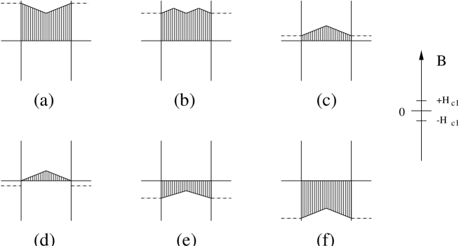
Fig. 6: Standard Bean profile of the flux density for the magnetization process in the hysteresis of a superconductor in the mixed state. The magnetization $M(H)$ is the integral of flux density in the sample.

For the following analysis we use the model of a superconducting slab which has a finite width along the $x$-axis and is infinite along the other two axes. Let us first study the standard behavior of the hysteresis, including the surface barrier effect of the lower critical field (or alternatively the Bean-Livingston barrier). We start by assuming

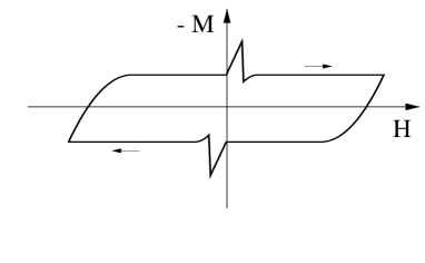
Fig. 7: Standard hysteresis in the mixed state of a superconductor based on the Bean critical state model.

that the external field was first raised to the maximum value $H_{m}$. Then the field distribution is similar to that in Fig. 6a). Now we turn the field off gradually and reverse it until we reach $-H_{m}$ (Fig. 6f). On the way the field distribution passes through the distributions shown in Fig. 6b)-e). It is important that in order to introduce reversed vortices into the system, the external field must exceed the lower critical field. Hence, in the range between $H_{\rm ext}=0$ and $-H_{c1}$, the internal flux distribution is unchanged, and at $-H_{c1}$ the magnetization jumps abruptly. After reaching $H_{\rm ext}=-H_{m}$, the field is again gradually turned to zero and further to $H_{m}$, so that the hysteresis cycle closes. The magnetization $M$ as a function of $H$ corresponds to the integrated flux density in the Bean critical state. The slope of the field distribution corresponds to the critical current ($J_{c}=(c/4\pi)\partial_{x}B_{z}$) and is proportional to the width of the hysteresis loop (Fig. 7).

If we now introduce domain walls as additional barriers within the sample, new structures appear in the hysteresis cycle. The domain wall is characterized by a specific barrier field (height) $B^{*}$; i.e., if the local field at the domain wall exceeds $B^{*}$, the domain wall is permeable to vortices. For simplicity we consider the case of two domain walls which fence in some region inside the slab. We start again from the situation in which the external field is at the value $H_{m}$, so that everywhere in the sample the local field value is larger than $B^{*}$, and the Bean profile has developed everywhere with a slope corresponding to the critical current due to usual pinning (Fig. 8a). Now, we gradually reduce the external field. As we reach zero, we find that the domain walls have trapped some flux; that is, more flux than usual is remaining in the sample (Fig. 8b). If we now turn to negative fields, then initially at $-H_{c1}$, reversed flux lines enter and annihilate the flux close to surface (Fig. 8c). With decreasing external field, the reversed flux lines reach the domain walls and annihilate vortices on the domain wall, which are in turn immediately replaced by new positive flux lines from the interior of the fenced in region. This process continues until the density of positive vortices on the domain wall is essentially zero and leads to a sharp increase in the magnetization similar to that at the lower critical field (Fig. 8d). Note that the negative vortices from the outside cannot enter the inner region yet, since at the end of this process the domain wall is occupied by reversed (negative) fractional vortices, which now provide a barrier. The flux density must be enhanced from outside, and the domain wall only becomes permeable when the local field of the negative vortices has reached $-B^{*}$ (Fig. 8e). Then, negative vortices can pass freely through the domain wall and annihilate the remaining positive vortices on the other side. This leads to a further avalanche-like rise in the magnetization. Then the external field is lowered until we reach $-H_{m}$ (Fig. 8f). The analogous continuation for increasing field finally leads to a closed hysteresis cycle.

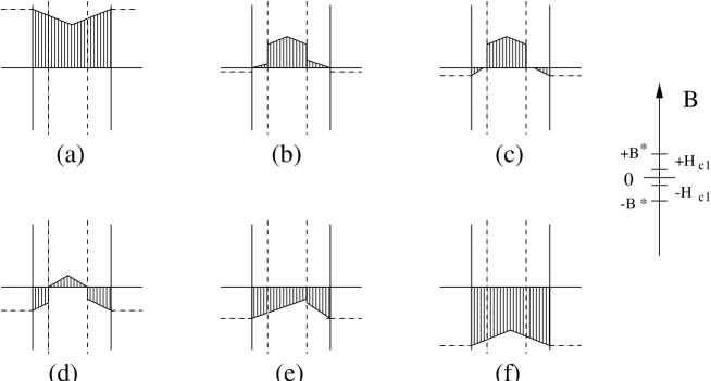
Fig. 8: Bean profile of a superconducting slab with two domain walls in a magnetic field. The critical field and the barrier field are indicated on the axis on the right hand side.

The additional sharp avalanche-like structures in the magnetization depend strongly on the position of the domain walls. As mentioned earlier, the domain walls

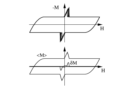
Fig. 9: Hysteresis of a superconducting slab containing domain walls as barriers. Upper figure: Several cycles with varying location of the domain wall. Lower figure: Average of several cycles and standard deviation, which possess maxima around the region of $\pm H_{c1}$.

are not rigidly fixed, but only pinned, and can change their position. During several cycles, the domain walls may be located at different places from cycle to cycle due to pressure from the vortices. Hence, the hysteresis cycles do not retrace themselves completely, but rather have strong deviations in the field range where the avalanche effects occur, i.e., close to the lower critical field, $\pm H_{c1}$. Taking the average over several cycles, the standard deviation, $\delta M=\langle(M(H)-\langle M(H)\rangle)^{2}\rangle$ reveals a strong “noise” signal, as shown in Fig. 9 ($\langle...\rangle$ denotes the average over many cycles). This noise is intrinsic to the superconducting state with internal barriers. It is easy to see that the magnitude of this noise depends on the barrier height given by $B^{*}$, and it should disappear, if $B^{*}$ goes to zero (the case of a completely permeable domain wall):

$$\delta M\propto B^{*}\delta x,$$ (4.1)

where $\delta x$ is the standard deviation of the domain wall positions, only weakly dependent on temperature.

We may compare this behavior now to the experiments done on UPt₃ by Shung et al.. [5] The features of the noise in the hysteresis are qualitatively very similar to those obtained in our simple simulation. In the high-temperature phase, the noise in the hysteresis cycle is small and featureless. However, simultaneously with the onset of the second transition, the intrinsic noise appears continuously and grows essentially linearly with $|T-T_{c2}|$ as we expect from Eq. (4.1). Within the cycle the noise appears in the same field range and with a similar structure, as in our simulation, i.e. around $H_{c1}$. This suggests that the continuous increase of the noise is very likely connected with the broken time-reversal symmetry below the second transition where the degeneracy of the superconducting phase allows for domain formation. The barrier height introduced by these domain walls increases as the order parameter of the low-temperature phase grows. A similar picture arises also from the measurement of flux motion in the low-temperature phase of U_1-xTh_xBe₁₃ by Zieve et al., [22] as mentioned above.

5 Conclusion

We have shown that domain walls in time-reversal symmetry-breaking superconductors can play an important role for the motion of flux lines. Under certain conditions, domain walls can accommodate flux lines whose flux is a fraction of the standard flux quantum. On such domain walls, conventional vortices can decay into two fractional vortices. If such fractional vortices line up, the domain wall becomes a very efficient barrier to vortices.

Evidence for this property of the domain wall is given by the absence of flux creep or in the intrinsic noise of the hysteresis cycle. [2, 3, 4, 5, 22] In the case of UPt₃ and U_1-xTh_xBe₁₃ experiments reveal a clear connection between the onset of the time-reversal symmetry-breaking in the low-temperature phase and the appearance of a new flux trapping mechanism. In Sr₂RuO₄ the drop of the creep rate is not connected with the onset of the time-reversal symmetry breaking phase. Rather the drop around 50 mK may be associated with a “transition” of the domain wall states. This may be associated with the multi-band nature of the superconducting state, which can lead to the temperature dependence of parameters like the anisotropy factor $\nu$, since the relative contribution to superconductivity by the different bands certainly varies with temperature. This case needs definitely further consideration. The barrier effect of domain walls does not, in general, influence the magnitude of the critical current $J_{c}$, which is related to ordinary impurity-induced pinning effects. Although the initial flux relaxation is vanishing in the low-temperature phase, $J_{c}$ remains finite and does not show any anomalous temperature dependence, indicating that the phenomena are not connected with a change in the pinning of individual vortices. We may take the observation of such flux flow phenomena as indirect evidence for the presence of domain walls. To this time in none of the above mentioned superconductors has the direct observation of the domain walls been reported. Clearly, the discovery of lined-up fractional vortices could be one direct experimental verification. Another proposal is based on the modification of the local quasiparticle density of states in the domain wall which may be observable by scanning tunneling microscopy. [14] This paper presents a plausible explanation for the basic properties seen in the experiments of three unconventional superconductors. Nevertheless, several details in the experimental data, which may be typical for the phenomenon or specific to each system, remain to be discussed in future.

References

- [1] G. Blatter, M. V. Feigel’man, V. B. Geshkenbein, A.I. Larkin and V. M. Vinokur, Rev. Mod. Phys. 66 (1994), 1125.
- [2] A. Amann, A.C. Mota, M. B. Maple and H. v.Löhneysen, Phys. Rev. B57 (1998), 3640.
- [3] E. Dumont, A.-C. Mota and J.L. Smith, Proceeding of LT22, (1999).
- [4] A.C. Mota, E. Dumont, A. Amann and Y. Maeno, Physica B 259-261 (1999), 934.
- [5] E. Shung, T. F. Rosenbaum and M. Sigrist, Phys. Rev. Lett. 80 (1998), 1078.
- [6] A.-C. Mota, G. Juri, P. Visani, A. Pollini, T. Teruzzi and K. Aupke, Physcia C 185-189 (1991), 343.
- [7] P. W. Anderson and Y. B. Kim, Rev. Mod. Phys. 36 (1964), 39.
- [8] M. Tinkham, Introduction to Superconductivity, (McGraw-Hill, 1996).
- [9] V. B. Geshkenbein and A. I. Larkin, Zh. Eksp. Teor. Fiz. 95 (1989), 1108 [Sov. Phys.-JETP 68 (1989), 639].
- [10] C. P. Bean, Rev. Mod. Phys. 36 (1964), 31.
- [11] M. Sigrist and K. Ueda, Rev. Mod. Phys. 63 (1991), 239.
- [12] G. E. Volovik and L. P. Gor’kov, Pis’ma Zh. Eksp. Teor. Fiz. 39 (1984), 550 [JETP Lett. 39 (1984), 674].
- [13] M. Sigrist, T. M. Rice and K. Ueda, Phys. Rev. Lett. 63 (1989), 1727.
- [14] M. Matsumoto and M. Sigrist, J. Phys. Soc. Jpn. 68 (1999), 994.
- [15] M. T. Heinilä and G. E. Volovik, Physica B210 (1995), 300.
- [16] M. Sigrist, D. B. Bailey and R. B. Laughlin, Phys. Rev. Lett. 74 (1995), 3249.
- [17] K. Kuboki and M. Sigrist, J. Phys. Soc. Jpn. 65 (1996), 361.
- [18] A. B. Kuklov, Phys. Rev. B52 (1995), R7002.
- [19] W. Belzig, C. Bruder and M. Sigrist, Phys. Rev. Lett. 80 (1998), 4285.
- [20] M. Sigrist, N. Ogawa and K. Ueda, J. Phys. Soc. Japan 60 (1991), 2341.
- [21] A.-C. Mota, private communication.
- [22] R. J. Zieve, T. F. Rosenbaum, J. S. Kim, G. R. Stewart and M. Sigrist, Phys. Rev. B51 (1995), 12041.