Instance Space of the Number Partitioning Problem

Abstract

Within the replica framework we study analytically the instance space of the number partitioning problem. This classic integer programming problem consists of partitioning a sequence of $N$ positive real numbers $\{a_{1},a_{2},\ldots,a_{N}\}$ (the instance) into two sets such that the absolute value of the difference of the sums of $a_{j}$ over the two sets is minimized. We show that there is an upper bound $\alpha_{c}N$ to the number of perfect partitions (i.e. partitions for which that difference is zero) and characterize the statistical properties of the instances for which those partitions exist. In particular, in the case that the two sets have the same cardinality (balanced partitions) we find $\alpha_{c}=1/2$. Moreover, we show that the disordered model resulting from the instance space approach can be viewed as a model of replicators where the random interactions are given by the Hebb rule.

I Introduction

Most statistical mechanics analyses of combinatorial optimization problems have concentrated on the characterization of average properties of minima of a given cost function [1, 2]. Usually, the cost function depends on a large set of fixed parameters, termed the instance of the optimization problem [e.g. the distances between cities in the celebrated travelling salesman problem (TSP)] which, in the framework of statistical mechanics, are treated as quenched random variables distributed according to some known probability distribution. Furthermore, in order to consider the subspace of configurations with a given average cost, one defines a probability distribution on the space of configurations (e.g. the $N!/2N$ different tours or ordering of the cities in the TSP), namely, the Gibbs distribution with ‘temperature’ $T=1/\beta$. The zero-temperature limit then singles out the configurations that minimize the cost function (ground states). Clearly, in this formulation the configurations are treated as fast, annealed variables.

Instead, in this work we explore the opposite viewpoint, namely, given a set of configurations we want to characterize the subspace of instances for which those configurations have a certain cost. This approach may be viewed as a best-case analysis in the sense that one searches for particularly easy instances that fit the given solutions. The situation here is similar to the physics approach to neural networks. In a first stage, attention was given to the neural dynamics while the coupling strengths between neurons were kept fixed according to some variant of the Hebb learning rule [3, 4]. (The neural dynamics itself can be viewed as a versatile heuristic in which the optimization problem is embedded in the neural couplings [5].) In the second stage which followed the seminal work of Gardner [6], the focus was on the characterization of the couplings distribution that ensures the stability of a given set of neural states. Gardner’s formulation allowed a rich interchange of concepts and methods between the statistical physics and the computational learning theory communities [7].

The specific optimization problem we consider in this paper is the number partition problem (NPP) [8, 9] which has received considerable attention in the physics literature recently [10, 11, 12]. It is stated as follows. Given a sequence of $N$ positive real numbers ${\bf a}=\{a_{1},a_{2},\ldots,a_{N}\}$ (the instance), the NPP consists of partitioning them into two disjoint sets ${\cal{A}}_{1}$ and ${\cal{A}}_{2}$ such that the difference

$$\mid\sum_{a_{j}\in{\cal{A}}_{1}}a_{j}-\sum_{a_{j}\in{\cal{A}}_{2}}a_{j}\mid$$ (1)

is minimized. Alternatively, we can search for the Ising spin configurations ${\bf s}=\{s_{1},\ldots,s_{N}\}$ that minimize the cost function

$$E\left({\bf s}\right)=~{}\mid\sum_{j=1}^{N}a_{j}s_{j}\mid,$$ (2)

where $s_{j}=1$ if $a_{j}\in{\cal{A}}_{1}$ and $s_{j}=-1$ if $a_{j}\in{\cal{A}}_{2}$. Despite its simplicity, the NPP was shown to belong to the NP-complete class, which basically means that there is no known deterministic algorithm guaranteed to solve all instances of this problem within a polynomial time bound [1].

In the proposed framework, we aim at characterizing the subspace of instances $\{{\bf a}\}$ for which the fixed set of partitions $\{{\bf s}^{l}\}~{}l=1,...,P,$ are perfect, i.e., $E\left({\bf s}^{l}\right)=0~{}\forall l$. To achieve this we define the energy in the instance space as

$${\cal H}\left({\bf a}\right)=\sum_{l=1}^{P}\left(\frac{1}{\sqrt{N}}\sum_{j=1}^{N}a_{j}s_{j}^{l}\right)^{2}$$ (3)

so that the $P$ partitions are perfect only if ${\cal H}=0$. Henceforth we will assume that $P$ increases linearly with $N$, i.e., $P=\alpha N$. Furthermore, we assume that the components $s_{j}^{l}$ are statistically independent random variables drawn from the probability distribution

$${\cal P}\left(s_{j}^{l}\right)=\frac{1}{2}\left(1+\frac{m}{\sqrt{N}}\right)\delta\left(s_{j}^{l}-1\right)+\frac{1}{2}\left(1-\frac{m}{\sqrt{N}}\right)\delta\left(s_{j}^{l}+1\right),$$ (4)

where the weights of the Dirac delta functions are chosen so that $\langle s_{j}^{l}\rangle=m/\sqrt{N}$. The motivation for this choice is twofold. First, the exhaustive search in the Ising configuration space for $N\leq 26$ as well as the analytical solution of the linear relaxation of the NPP indicate that the average difference between the cardinalities of sets ${\cal{A}}_{1}$ and ${\cal{A}}_{2}$,

$$\hat{m}=\frac{1}{N}~{}\sum_{j=1}^{N}s_{j},$$ (5)

vanishes like $1/\sqrt{N}$ for large $N$ [12]. Second, this scaling yields a non-trivial thermodynamic limit, $N\rightarrow\infty$, for the average free-energy density associated to the Hamiltonian (3).

In this paper we will apply standard statistical mechanics techniques to study analytically the ground states of the Hamiltonian (3). We concentrate our analysis on the zero-energy instances (i.e., instances for which perfect partitions exist) only, since the properties of the non-zero energy instances depend strongly on the rather arbitrary choice of the energy (3). Moreover, perfect partitions are important from a practical viewpoint as they may have code-breaking implications [13] and so it may be of interest to estimate the maximum number of perfect partitions that can be encoded in an arbitrary instance, as well as to characterize those instances that maximize the number of coded perfect partitions.

The rest of this paper is organized in the following way. In Sec.  II we use the replica method to evaluate the average free-energy density in the thermodynamic limit and to derive the replica-symmetric order parameters that describe the statistical properties of the instance space. In particular, we show that there is a critical value, $\alpha_{c}\left(m\right)N$, which limits the number of perfect partitions. Also in that section, we study the stability of the replica-symmetric solution against replica symmetry breaking and show that the zero-energy instances can reliably be described by the replica-symmetric order parameters. In Sec.  III we calculate the probability density for a given entry, say $a_{k}$, to have value $a$. This is achieved by integrating the joint probability distribution (the Gibbs distribution) over all entries except $a_{k}$. Finally, in Sec. IV we present some concluding remarks. In particular we show that the disordered model considered here is formally identical to a model of replicators with the random interactions given by the Hebb rule.

II Replica approach

Following the standard prescription of performing quenched averages on extensive quantities only [2], we define the average free-energy density $f$ as

$$-\beta f=\lim_{N\rightarrow\infty}\frac{1}{N}\left\langle\ln Z\right\rangle$$ (6)

where

$$Z=\int_{0}^{\infty}\prod_{j}da_{j}\delta\left(R-\frac{1}{N}\sum_{j}a_{j}\right)\mbox{e}^{-\beta{\cal H}\left({\bf a}\right)}$$ (7)

is the partition function and $\beta=1/T$ is the inverse temperature. Taking the limit $T\rightarrow 0$ in Eq. (7) ensures that only the instances that minimize ${\cal H}\left({\bf a}\right)$ will contribute to $Z$. Here $\langle\ldots\rangle$ stands for the average over the partitions ${\bf s}^{l}~{}(l=1,\ldots,P)$. The constraint on the mean of the instance vector is needed in order to exclude the trivial solution ${\bf a}=0$. Fortunately, the arbitrary parameter $R$ does not play any relevant role in the theory, giving only the scale of the order parameters of the model.

As usual, the quenched average in Eq. (6) is evaluated through the replica method: using the identity

$$\left\langle\ln Z\right\rangle=\lim_{n\rightarrow 0}\frac{1}{n}\ln\left\langle Z^{n}\right\rangle$$ (8)

we first evaluate $\left\langle Z^{n}\right\rangle$ for integer $n$ and then analytically continue to $n=0$. Using standard techniques [14] we obtain, in the thermodynamic limit

$$-\beta f = \lim_{n\rightarrow 0}\frac{1}{n}\mbox{extr}\{\frac{R^{2}}{2}\sum_{\rho}Q_{\rho}\hat{Q}_{\rho}-R^{2}\sum_{\rho<\delta}q_{\rho\delta}\hat{q}_{\rho\delta}$$ (11)

$$\mbox{}+R\sum_{\rho}\hat{R}_{\rho}+\alpha\ln G_{1}\left(q_{\rho\delta},Q_{\rho}\right)$$

$$\mbox{}+\ln G_{2}\left(\hat{q}_{\rho\delta},\hat{R}_{\rho},\hat{Q}_{\rho}\right)\}$$

where

$$G_{1} = \int_{-\infty}^{\infty}\prod_{\rho}\frac{d\tilde{x}_{\rho}}{\sqrt{2\pi}}\exp\left[-\frac{1}{2}\sum_{\rho}\left(1+2\beta R^{2}Q_{\rho}\right)\tilde{x}_{\rho}^{2}\right.$$ (13)

$$\left.-2\beta R^{2}\sum_{\rho<\delta}\tilde{x}_{\rho}\tilde{x}_{\delta}q_{\rho\delta}+~{}im\sqrt{2\beta R^{2}}\sum_{\rho}\tilde{x}_{\rho}\right]$$

and

$$G_{2}=\int_{0}^{\infty}\prod_{\rho}da_{\rho}\exp\left(-\frac{1}{2}\sum_{\rho}\hat{Q}_{\rho}a_{\rho}^{2}+\sum_{\rho<\delta}\hat{q}_{\rho\delta}a_{\rho}a_{\delta}\right.$$ (14)

$$\left.-\sum_{\rho}\hat{R}_{\rho}a_{\rho}\right).$$ (15)

The extremum in Eq. (11) is taken over all order parameters $\left(\hat{q}_{\rho\delta},\hat{R}_{\rho},\hat{Q}_{\rho},q_{\rho\delta},Q_{\rho}\right)$. The physical order parameters

$$q_{\rho\delta}=\left\langle\frac{1}{NR^{2}}\sum_{i=1}^{N}\left\langle a_{i}^{\rho}\right\rangle_{T}\left\langle a_{i}^{\delta}\right\rangle_{T}\right\rangle~{}~{}~{}~{}~{}\rho<\delta,$$ (16)

and

$$Q_{\rho}=\left\langle\frac{1}{NR^{2}}\sum_{i=1}^{N}\left\langle\left(a_{i}^{\rho}\right)^{2}\right\rangle_{T}\right\rangle$$ (17)

measure the overlap between a pair of different equilibrium instances ${\bf a}^{\rho}$ and ${\bf a}^{\delta}$, and the overlap of an equilibrium instance ${\bf a}^{\rho}$ with itself, respectively. Here, $\langle\ldots\rangle_{T}$ stands for a thermal average.

A Replica-symmetric solution

To proceed further we make the replica symmetric ansatz, i.e., we assume that the values of the order parameters are independent of their replica indices

$$q_{\rho\delta}=q$$ and

and

.

(18)

Evaluation of Eqns. (13) and (14) with this ansatz is straightforward. In order to write the replica symmetric average free-energy density it is convenient to introduce the new variables

$$\eta=R^{2}\left(\hat{Q}+\hat{q}\right),~{}~{}~{}~{}\tau=\frac{\hat{R}}{\sqrt{2\left(\hat{Q}+\hat{q}\right)}},~{}~{}~{}~{}\theta=\frac{\hat{q}}{2\left(\hat{Q}+\hat{q}\right)},$$ (19)

and rescale the temperature $\beta^{\prime}=\beta R^{2}$ so that

$$-\frac{\beta^{\prime}}{R^{2}}f_{rs} = \frac{1}{2}\ln\left(\frac{\pi R^{2}}{2}\right)+\frac{1}{2}\eta\left[Q-2\theta\left(Q-q\right)\right]+\tau\sqrt{2\eta}$$ (22)

$$-\frac{\alpha}{2}\ln\left[1+2\beta^{\prime}\left(Q-q\right)\right]-\beta^{\prime}\alpha\frac{m^{2}+q}{1+2\beta^{\prime}\left(Q-q\right)}$$

$$-\frac{1}{2}\ln\eta+\int_{-\infty}^{\infty}Dz\ln\left(\mbox{e}^{\Xi_{z}^{2}}\mbox{erfc}\Xi_{z}\right)$$

where

$$\Xi_{z}=\tau+z\theta^{1/2},$$ (23)

and

$$Dz=\frac{dz}{\sqrt{2\pi}}\mbox{e}^{-z^{2}/2}$$ (24)

is the Gaussian measure. Thus it is clear from Eq. (22) that the parameter $R$ yields the scales of the temperature and free-energy, not affecting in any significant way the physical, replica-symmetric order parameters

$$q=\left\langle\frac{1}{NR^{2}}\sum_{i=1}^{N}\left\langle a_{i}\right\rangle_{T}^{2}\right\rangle,$$ (25)

and

$$Q=\left\langle\frac{1}{NR^{2}}\sum_{i=1}^{N}\left\langle a_{i}^{2}\right\rangle_{T}\right\rangle.$$ (26)

The replica-symmetric average energy density $\epsilon_{rs}=\partial\left(\beta f_{rs}\right)/\partial\beta$ is given by

$$\epsilon_{rs}/\alpha R^{2}=\frac{q+m^{2}}{\left[1+2\beta^{\prime}\left(Q-q\right)\right]^{2}}+\frac{Q-q}{1+2\beta^{\prime}\left(Q-q\right)}$$ (27)

which vanishes in the limit $\beta^{\prime}\rightarrow\infty$ provided that $q<Q$.

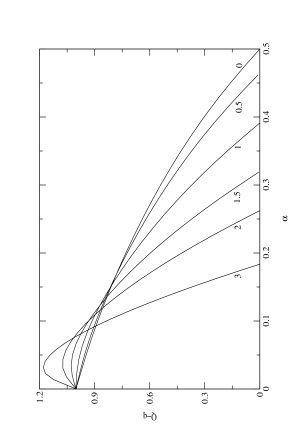
FIG. 1.: Average variance of the zero-energy instance entries $Q-q$ as a function of $\alpha$ for $m=0$, $0.5$, $1$, $1.5$, $2$, and $3$. The value of $\alpha$ at which the variance vanishes($\alpha_{c}$) gives an upper bound to the number of perfect partitions.

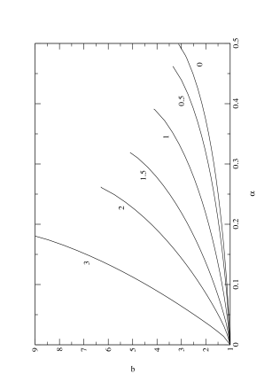
FIG. 2.: Average overlap between two different zero-energy instances $q$ as a function of $\alpha$ for $m=0$, $0.5$, $1$, $1.5$, $2$, and $3$. The curves end at $\alpha=\alpha_{c}$.

As justified in Sec. I we will focus on this limit only. After some algebra, the saddle-point equations in this limit are written as

$$\theta=\frac{q+m^{2}}{2\left(Q-q\right)}~{},$$ (28)

$$\eta=\frac{\alpha}{Q-q}~{},$$ (29)

$$\tau=\sqrt{\frac{Q-q}{2\alpha}}\left(1-\alpha+\frac{\alpha m^{2}}{Q-q}\right)~{},$$ (30)

$$\sqrt{2\eta}=-2\tau+\frac{2}{\sqrt{\pi}}\int_{-\infty}^{\infty}Dz~{}\frac{\exp\left(-\Xi_{z}^{2}\right)}{\mbox{erfc}\Xi_{z}}~{},$$ (31)

$$\eta\left(Q-q\right)=1-\frac{1}{\sqrt{\pi\theta}}\int_{-\infty}^{\infty}Dz~{}z~{}\frac{\exp\left(-\Xi_{z}^{2}\right)}{\mbox{erfc}\Xi_{z}}~{},$$ (32)

with $\Xi_{z}$ given by Eq. (23). In general these equations can be solved numerically only. In Figs. 1 and 2 we present the dependence of $Q-q$ and $q$, respectively, on $\alpha$ for different values of $m$. For $\alpha=0$ we find $Q-q=q=1$, $\theta=(1+m^{2})/2$, and $\eta=0$, while $\tau$ diverges like $1/\sqrt{2\alpha}$. According to the physical meaning of the order parameters given in Eqns. (25) and (26), the difference $Q-q$ measures the average variance of the zero-energy instance entries: the larger this difference, the larger the dispersion of the instance entries. Interestingly, for fixed $m>0$ this variance reaches its maximum for $\alpha>0$. The divergence of the order parameters $Q$ and $q$ (and of their difference, as well), for $m\rightarrow\infty$ and $\alpha\neq 0$ is expected, since in order that an extremely unbalanced partition become a perfect partition there must exist some very large entries to compensate for the much larger number of entries in one of the sets. Moreover, we observe from Fig. 1 that for fixed $m$ there is a value of $\alpha=\alpha_{c}$ at which the overlap between two zero-energy instances $q$ equals its maximal value $Q$. This results signals the shrinking of the zero-energy instance subspace to instances differing from a microscopic number of entries $a_{j}$ only. Besides, it gives the limit of existence of the solutions with zero-energy: for $\alpha>\alpha_{c}$ there are no zero-energy instances. Taking the limit $q\rightarrow Q$ in the saddle-point equations (28 - 32) yields

$$\alpha_{c}=1-\int_{-\Delta}^{\infty}Dz$$ (33)

where

$$\Delta=\left(\frac{\alpha_{c}m^{4}}{Q_{c}+m^{2}}\right)^{\frac{1}{2}}$$ (34)

is the solution of

$$\frac{\Delta}{m^{2}}=\int_{-\Delta}^{\infty}Dz\left(z+\Delta\right)-\Delta.$$ (35)

Here $Q_{c}$ stands for the order parameter $Q$ evaluated at $\alpha_{c}$. For $m=0$ we can solve these equations analytically: we find that $\Delta$ vanishes like $m^{2}/\sqrt{2\pi}$ and so $\alpha_{c}=1/2$ and $Q_{c}=\pi$.

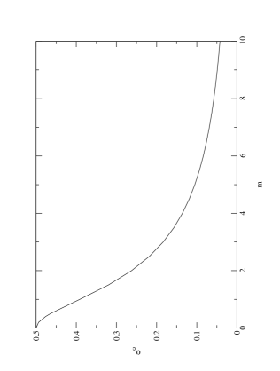
FIG. 3.: Instance independent upper bound to the number of perfect partitions $\alpha_{c}$ as a function of the parameter $m$ which measures the unbalance of the partitions. For balanced partitions ($m=0$) we find $\alpha_{c}=1/2$.

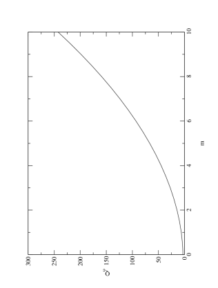
FIG. 4.: Average overlap of a zero-energy instance with itself calculated at $\alpha_{c}$ as a function of $m$. For balanced partitions ($m=0$) we find $Q_{c}=\pi$.

In Figs. 3 and 4 we show $\alpha_{c}$ and $Q_{c}$, respectively, as functions of $m$. The dependence of $\alpha_{c}$ on $m$ indicates that instances for which there are an extensive number of unbalanced perfect partitions become very rare with increasing $m$. In particular, there are no zero-energy instances for partitions with average cardinalities difference [see Eq. (5)] of order of $1$.

B Stability analysis

The condition for the local stability of the replica-symmetric saddle-point is given by [14]

$$\alpha\gamma_{1}\gamma_{2}\leq 1$$ (36)

where $\gamma_{1}$ and $\gamma_{2}$ are the transverse eigenvalues [15] of the matrices of second derivatives of $G_{1}$ and $G_{2}$ with respect to $q_{\rho\delta}$ and $\hat{q}_{\rho\delta}$, respectively, evaluated at the replica-symmetric saddle-point. After some algebra we find that condition (36) reduces to

$$\alpha\,\left[\eta\left(Q-q\right)\right]^{-2}\int_{-\infty}^{\infty}Dz\left({\overline{a^{2}}}-{\overline{a}}^{2}\right)^{2}\leq 1$$ (37)

where

$${\overline{a^{n}}}=\frac{\int_{0}^{\infty}da\;a^{n}\exp\left(-\frac{1}{2}a^{2}-a\;\sqrt{2}\;\Xi_{z}\right)}{\int_{0}^{\infty}da\exp\left(-\frac{1}{2}a^{2}-a\;\sqrt{2}\;\Xi_{z}\right)}.$$ (38)

Taking the limit $q\rightarrow Q$ we can easily show that

$$\eta\left(Q-q\right)\rightarrow\alpha_{c}$$ (39)

and

$$\int_{-\infty}^{\infty}Dz\left({\overline{a^{2}}}-{\overline{a}}^{2}\right)^{2}\rightarrow\alpha_{c},$$ (40)

with $\alpha_{c}$ given by Eq. (33), so that the left hand side of Eq. (37) equals $1$ at $\alpha=\alpha_{c}$. Moreover, we have verified numerically that this stability condition is always satisfied for $\alpha<\alpha_{c}$.

III Probability distribution of entries

The traditional probabilistic approach to study optimization problems introduces a probability distribution over the space of instances. The main objection to this approach is that one rarely knows what probability distribution is realistic. In the NPP, for instance, it is usually assumed that the entries $a_{k}$ are statistically independent random variables distributed uniformly in the unit interval [8, 9, 10]. In this section we calculate analytically the distribution of probability that a certain entry, say $a_{k}$, of a zero-energy instance assumes the value $a$, defined by

$${\mathcal{P}}_{k}\left(a\right) = \lim_{\beta\rightarrow\infty}\left\langle~{}\left\langle\delta\left(a_{k}-a\right)\right\rangle_{T}~{}\right\rangle=\lim_{\beta\rightarrow\infty}\left\langle~{}\frac{1}{Z}\int_{0}^{\infty}\prod_{j}da_{j}\right.$$ (42)

$$\left.\delta\left(R-\frac{1}{N}\sum_{j}a_{j}\right)\ \delta\left(a_{k}-a\right)\mbox{e}^{-\beta{\cal H}\left({\bf a}\right)}\right\rangle$$

where $Z$ and ${\cal H}$ are given by Eqns. (7) and (3), respectively. As all entries are equivalent we can write ${\mathcal{P}}_{k}\left(a\right)={\mathcal{P}}\left(a\right)\forall k$. Hence to evaluate Eq. (42) we introduce the auxiliary energy

$${\cal H}_{aux}\left({\bf a}\right)={\cal H}\left({\bf a}\right)+h\sum_{k}\delta\left(a_{k}-a\right),$$ (43)

so that

$${\mathcal{P}}\left(a\right)=-\lim_{\beta\rightarrow\infty}~{}\frac{1}{N\beta}\left.\frac{\partial\langle\ln Z_{aux}\rangle}{\partial h}\right|_{h=0}$$ (44)

where $Z_{aux}$ is the partition function (7) with ${\cal H}$ replaced by ${\cal H}_{aux}$. Of course, we note that the entries $\left(a_{1},\ldots,a_{N}\right)$ are not statistically independent and their joint probability distribution is simply the Gibbs probability distribution

$${\mathcal{W}}\left({\bf a}\right)=\frac{1}{Z}\exp\left[-\beta{\cal H}\left({\bf a}\right)\right].$$ (45)

As expected, Eq. (42) is recovered by integrating this joint distribution over $a_{j}$ for all $j\neq k$ and then setting $a_{k}=a$. Using Eq. (44) the calculations needed to evaluate ${\mathcal{P}}\left(a\right)$ become analogous to those used in the evaluation of the free-energy density (11). Within the replica-symmetric framework and in the limit $\beta\rightarrow\infty$ with $q<Q$ the final result is

$${\mathcal{P}}\left(a\right)=\sqrt{\frac{2\eta}{\pi R^{2}}}~{}\int_{-\infty}^{\infty}Dz~{}\frac{1}{\mbox{erfc}\,\Xi_{z}}~{}\exp\left[-\frac{\eta}{2R^{2}}~{}a^{2}\right.$$ (46)

$$\left.-a\Xi_{z}\,\left(\frac{2\eta}{R^{2}}\right)^{1/2}-\Xi_{z}^{2}\right]~{}~{}~{}~{}~{}~{}a\geq 0,~{}~{}~{}~{}~{}~{}~{}~{}~{}~{}~{}~{}~{}$$ (47)

which for $\alpha=0$ reduces to

$${\mathcal{P}}\left(a\right)=\frac{1}{R}\,\exp\left(-\frac{a}{R}\right)~{}~{}a\geq 0.$$ (48)

To handle a possible singularity in the limit $q\rightarrow Q$ it is more convenient to consider instead the cumulative distribution function defined by

$${\mathcal{C}}\left(a\right) = \int_{0}^{a}da^{\prime}\,{\mathcal{P}}\left(a^{\prime}\right)$$ (49)

$$= 1-\int_{-\infty}^{\infty}Dz~{}\frac{\mbox{erfc}\left[\Xi_{z}+a\left(\eta/2R^{2}\right)^{1/2}\right]}{\mbox{erfc}\,\Xi_{z}}.$$ (50)

Taking the limit $q\rightarrow Q$ yields

$${\mathcal{C}}_{c}\left(a\right)=1-\frac{1}{2}\mbox{erfc}\left[\frac{\Delta}{\sqrt{2}}\left(1+\frac{a}{Rm^{2}}\right)\right]$$ (51)

where $\alpha_{c}$ and $\Delta$ are given by Eqns. (33) and (35), respectively. The interesting feature of this distribution is that ${\mathcal{C}}_{c}\left(0\right)$ is non-zero indicating thus that the probability distribution (46) evaluated at $\alpha=\alpha_{c}$ has a delta peak in $a=0$. Explicitly,

$${\mathcal{P}}_{c}\left(a\right)={\mathcal{C}}_{c}\left(0\right)\,\delta\left(a\right)+\frac{d{\mathcal{C}}_{c}}{da}~{}~{}~{}a\geq 0,$$ (52)

which for $m=0$ reduces to

$${\mathcal{P}}_{c}\left(a\right)=\frac{1}{2}\,\delta\left(a\right)+\frac{1}{\sqrt{4\pi R^{2}}}\exp\left(-\frac{a^{2}}{4R^{2}}\right)~{}~{}~{}a\geq 0.$$ (53)

In Fig. 5 we show the cumulative distribution function $C(a)$ for $m=0$ and several values of $\alpha$. We note that $C(0)\neq 0$ only at $\alpha=\alpha_{c}$.

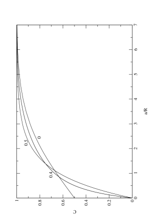
FIG. 5.: Cumulative distribution function of the zero-energy instance entries for $m=0$ and $\alpha=0$, $0.4$, and $0.5$. Note that $C(0)\neq 0$ only at $\alpha=\alpha_{c}=0.5$.

IV Conclusion

Since the instance entries are continuous variables $a_{i}\in\left[0,\infty\right)~{}\forall i$ we can resort to a simple gradient descent algorithm to find the minima of the energy ${\mathcal{H}}\left({\mathbf{a}}\right)$, defined by Eq. (3), which have a given mean. More pointedly, it can be easily verified that the dynamics

$$\frac{da_{k}}{dt}=-a_{k}\left[\frac{1}{N}\sum_{l=1}^{P}s_{k}^{l}\sum_{i=1}^{N}s_{i}^{l}a_{i}-\frac{1}{NR}{\mathcal{H}}\left({\mathbf{a}}\right)\right]~{}\forall k$$ (54)

minimizes ${\mathcal{H}}\left({\mathbf{a}}\right)$ while the mean $\sum_{i}a_{i}$ is a constant of motion. Interestingly, Eq. (54) is readily recognized as a particular realization of the classical replicator equation which has been used to describe the evolution of self-reproducing entities (replicators) in a variety of fields, such as game theory, prebiotic evolution and sociobiology, to name only a few [16]. In fact, $a_{i}$ can be viewed as the concentration of species $i$ whose fitness ${\mathcal{H}}_{i}$ is the derivative ${\mathcal{H}}_{i}=\partial{\mathcal{H}}/\partial a_{i}$ of a fitness functional ${\mathcal{H}}\left({\mathbf{a}}\right)$. The (infinite) population of replicators is composed of $N$ different species which evolve under the constraint of constant total concentration. The disordered model considered here is a variant of the model of replicators with random interactions studied by Diederich and Opper [17] (see also [18]) in which the fitness functional is given by

$${\mathcal{H}}_{DO}\left({\mathbf{a}}\right)=\sum_{ij}J_{ij}a_{i}a_{j}$$ (55)

where the couplings $J_{ij}=J_{ji}~{}\left(i\neq j\right)$ are independent, identically distributed Gaussian random variables with mean zero and variance $1/N$, while the self-interactions are non-random, species independent control parameters of the model, i.e., $J_{ii}=u~{}\forall i$. Clearly, the energy given by Eq. (3) can be rewritten in the form of Eq. (55) with the couplings given by the Hebb rule $J_{ij}=\frac{1}{N}\sum_{l}^{P}s_{i}^{l}s_{j}^{l}$ [3]. We note that in our model the self-interaction is $J_{ii}=\alpha~{}\forall i$, while the mean and variance of the off diagonal couplings are $\alpha m^{2}/N\rightarrow 0$ and $\alpha\left(1-m^{4}/N^{2}\right)/N\rightarrow\alpha/N$, respectively. Moreover, as in the Hopfield model [3], though the $s_{i}^{l}$ are independent random variables, the couplings $J_{ij}$ are not. It is interesting thus to interpret our results in the light of the random replicator model: for $\alpha<\alpha_{c}$ the global optimum of the fitness functional, ${\mathcal{H}}\left({\mathbf{a}}\right)=0$, can be reached with the coexistence of all species; for $\alpha=\alpha_{c}$ reaching that optimum requires the extinction of a macroscopic number of species, as signaled by the delta peaks in $a=0$; and for $\alpha>\alpha_{c}$ the interactions between species are such that the optimum is never reached.

To conclude, we mention that while the traditional approach of Computer Science to the validation of combinatorial search algorithms focuses almost exclusively on the instance space (e.g. the worst-case analysis is basically a search for instances that give the poorest performance of the algorithm under study [1]), the statistical mechanics approach has concentrated mainly on the configuration space, with the instances being drawn from arbitrary probability distributions [2]. Building on the work of Gardner on neural networks [6], we illustrate in this paper the usefulness of equilibrium statistical mechanics tools to investigate the statistical properties of the instance space as well. For the optimization problem we have considered, namely, the number partitioning problem, we have searched the instance space for the best (easiest) instances to show that there is a maximum number of uncorrelated perfect partitions, $\alpha_{c}\left(m\right)N$ (see Fig. 3). In particular, for balanced partitions ($m=0$) we find $\alpha_{c}(0)=1/2$. Clearly, this result yields an upper bound to the number of perfect partitions (ground-state degeneracy) that can be found for any arbitrary instance. As in the neural networks case, the instance space analysis proposed in this paper can be extended to virtually all optimization problems.

We thank Pablo Moscato for illuminating conversations. The work of JFF was supported in part by Conselho Nacional de Desenvolvimento Científico e Tecnológico (CNPq). FFF is supported by FAPESP.

REFERENCES

- [1] M. R. Garey and D. S. Johnson, Computers and Intractability: A Guide to the Theory of NP-Completeness (Freeman, San Francisco, 1979).
- [2] M. Mézard, G. Parisi and M. A. Virasoro, Spin Glass Theory and Beyond (World Scientific, Singapore, 1987).
- [3] J. J. Hopfield, Proc. Natl. Acad. Sci. USA 79, 2554 (1982).
- [4] D. J. Amit, H. Gutfreund and H. Sompolinsky, Ann. Phys. 173, 30 (1987).
- [5] J. J. Hopfield and D. W. Tank, Biol. Cybern. 52, 141 (1985).
- [6] E. Gardner, J. Phys. A 21, 257 (1988).
- [7] T. L. H. Watkin, A. Rau and M. Biehl, Rev. Mod. Phys. 65, 499 (1993).
- [8] N. Karmakar, R. M. Karp, G. S. Lueker and A. M. Odlyzko, J. Appl. Prob. 23, 626 (1986).
- [9] D. S. Johnson, C. R. Aragon, L. A. McGeoch and C. Schevon, Operations Research 39, 378 (1991).
- [10] F. F. Ferreira and J. F. Fontanari, J. Phys. A 31, 3417 (1998).
- [11] S. Mertens, Phys. Rev. Lett. 81, 4281 (1998).
- [12] F. F. Ferreira and J. F. Fontanari, Physica A 269, 58 (1999)
- [13] A. Shamir, Proceedings 11th Annual ACM Symposium on Theory of Computing. Association for Computing Machinery, New York, pp. 118-129 (1979).
- [14] E. Gardner and B. Derrida, J. Phys. A 21, 271 (1988).
- [15] J. R. L. Almeida and D. J. Thouless, J. Phys. A 11 983 (1978)
- [16] P. Schuster and K. Sigmund, J. Theor. Biol 100 533 (1983)
- [17] S. Diederich and M. Opper, Phys. Rev. A 39 4333 (1989)
- [18] P. Biscari and G. Parisi, J. Phys. A 28 4697 (1995)