A New Vortex Solution for Two-Component Nonlinear Schrödinger Equation in Anisotropic Optical Media

Abstract

A theoretical study is given of a new type of optical vortex in nonlinear anisotropic media. This is realized as a special solution of the two-component non-linear Schrödinger equation. The vortex is inherent in the spin texture that is caused by an anisotropy of dielectric tensor, for which a role of spin is played by the Stokes vector (or pseudo-spin). By using the effective Lagrangian for the pseudo-spin field, we give an explicit form for the vortex solution for the case of two types of optical anisotropy; that is, nonlinear counterpart of birefringence giving rise to the Faraday and Cotton-Mouton effects. We also examine the evolution equation of the new vortex with respect to the propagation direction.

Nonlinear optics has been a major subject in physics for long time [1]. The main interest is focussed on particular solutions of the basic non-linear equation that governs the light field or electromagnetic field. Among others, remarkable is an optical vortex, the existence of which has been early suggested in [1]. Recently the detailed study has been carried out from both of theoretical and experimental point of view [2, 3]. More recently experimental verification has been also given for the multi-vortices [4]. The basic idea of the optical vortex follows an analogy with the superfluid vortex that is described by the complex order parameter for bose fluid[3], namely, the equation for the light field, which is known as the nonlinear Schrödinger equation (NLS), is very similar to the Pitaevki equation. Thus it is natural to expect the occurrence of the optical counterpart of the superfluid vortex.

The purpose of this letter is to explore a possible new type of vortex in nonlinear and anisotropic media that are characterized by a variant of birefringence. We call this new type vortex an “optical spin vortex”. Our starting equation is the two-component NLS. The two-component NLS has been recently used for exploring an object of dynamic soliton [5], which is the two modes induced waveguide leading to the soliton polarization dynamics. This work shares partly the basic idea with the present attempt in the point that two component NLS naturally incorporates the polarization state of light. Indeed the concept of polarization plays an important role in modern optics, especially in crystal optics [6, 7]. The quantity describing the polarization state is realized by the Stokes parameters, which forms a pseudo-spin and is geometrically described by a point on the Poincaré sphere. Thus the two component NLS can be written in terms of the field of pseudo-spin, which is naturally achieved by introducing the effective “Lagrangian” of fluid dynamical form. The use of the effective Lagrangian gives us a direct access to the analysis of the optical spin vortex. The main thrust is twofold: First we give an explicit form for the vortex solution by adopting some specific nonlinear birefringence; the concrete form is given by the nonlinear counterpart of the one causing the Faraday and Cotton-Mouton effects. This will be carried out by numerical way. We next examine the evolutional behavior of a vortex with respect to the direction of the wave propagation.

Two component nonlinear Schrödinger equation.—

First we derive the two-component NLS for the light wave traveling through anisotropic media. The procedure follows the one developed in a recent paper [8]. Suppose that the electromagnetic wave of wave vector $k$ travels in the direction of $z$ with the dielectric tensor $\hat{\epsilon}$. The nonlinear nature of media implies that $\hat{\epsilon}$ has a field dependence in nonlinear form, the explicit form of which will be given later. Further we assume that $\hat{\epsilon}$ varies slowly compared with the wavenumber $k$. The $z$-axis is chosen as a principal axis of the dielectric tensor, namely, the axis corresponding to one of the eigenvalues of the dielectric tensor. In this geometry, $\hat{\epsilon}$ is taken to be $2\times 2$ matrix. Let us consider the field equation for the displacement field ${\bf D}$, which is reduced from the Maxwell equation [5, 9]:

$${\partial^{2}{\bf D}\over\partial z^{2}}+\nabla^{2}{\bf D}+\left({\omega\over c}\right)^{2}\hat{\epsilon}{\bf D}=0$$ (1)

where $\nabla=\left({\partial\over\partial x},\;{\partial\over\partial y}\right)$ and $(x,y)$ denotes the coordinate in the plane perpendicular to $z$ axis. Now we put

$${\bf D}(x,y,z)={\bf f}(x,y,z)\exp[ikn_{0}z]$$ (2)

with $k={\omega\over c}$, and $n_{0}(\equiv\sqrt{\epsilon_{0}})$ means the refractive index for the case as if the medium is isotropic. The amplitude ${\bf f}(x,y,z)$ is written as ${\bf f}={}^{t}(f_{1},f_{2})=f_{1}{\bf e}_{1}+f_{2}{\bf e}_{2}$. We assume that ${\bf f}$ is slowly varying function of $z$ besides $(x,y)$, and ${\bf e}_{1}$ and ${\bf e}_{2}$ denotes the basis of linear polarization. By substituting (2) into (1) and noting the slowly varying nature of ${\bf f}$ i.e., $\left|{\partial{\bf f}\over\partial z}\right|\ll k|{\bf f}|$, we can derive the equation for the amplitude ${\bf f}$, namely, we can only retain the first derivative ${\partial{\bf f}\over\partial z}$ as well as the Laplacian with respect to $(x,y)$ [10], hence

$$i\lambda{\partial{\bf f}\over\partial z}+\left[{\lambda^{2}\over n_{0}^{2}}\nabla^{2}+\left(\hat{\epsilon}-n_{0}^{2}\right)\right]{\bf f}=0$$ (3)

where $\lambda$ is the wavelength divided by $2\pi$. This equation is regarded as a two-state Schrödinger equation where $\lambda$ just corresponds to the Planck constant and $z$ plays a role of time variable. The components $(f_{1},f_{2})$ couple each other to give rise to the change of polarization which is just the effect of birefringence governed by a $2\times 2$ matrix “potential” $\hat{v}=\hat{\epsilon}-n_{0}^{2}$. $\hat{v}$ represents a deviation from the isotropic value and it becomes hermitian if the non-absorptive medium is concerned. From the hermiticity, the most general form of $\hat{v}$ is written as

$${\hat{v}}=\left(\begin{array}[]{cc}v_{0}+\alpha&\beta+i\gamma\\ \beta-i\gamma&v_{0}-\alpha\end{array}\right).$$ (4)

For later convenience, we transform the basis to the circular basis instead of the linear polarization (${\bf e}_{1},\,{\bf e}_{2})$, that is, ${\bf e_{\pm}}=\left(1/{\sqrt{2}}\ \right)({\bf e}_{1}\pm i{\bf e}_{2})$, which is written as $({\bf e}_{+},\,{\bf e}_{-})=T({\bf e}_{1},{\bf e}_{2})$. Here $T$ is given by $2\times 2$ unitary matrix:

$$T={1\over\sqrt{2}}\left(\begin{array}[]{cc}1&i\\ 1&-i\end{array}\right).$$ (5)

By introducing the wave function as $\psi=T{\bf f}={}^{t}\left(\psi_{1}^{*},\,\psi_{2}^{*}\right)$, we have the Schrödinger equation for $\psi$:

$$i\lambda{\partial\psi\over\partial z}=\hat{H}\psi$$ (6)

with the transformed “Hamiltonian”

$$\hat{H}=ThT^{-1}=-{\lambda^{2}\over n_{0}}\nabla^{2}+V.$$ (7)

The “field-dependent” potential $V$ is written in terms of the Pauli spin; $V=v_{0}\times 1+\sum_{i=1}^{3}v_{i}\sigma_{i}$.

Effective Lagrangian for the pseudo-spin field.—

We now introduce the “quantum” Lagrangian leading to the Schrödinger type equation, which is given by

$$I=\int\psi^{\dagger}\left(i\lambda{\partial\over\partial z}-\hat{H}^{\prime}\right)\psi d^{2}xdz.$$ (8)

Indeed, the Dirac variation equation $\delta I=0$ recovers the Scrödinger equation. We write $L_{C}=\int\psi^{\dagger}i\lambda{\partial\over\partial z}\psi d^{2}x$ and $H=\int\psi^{\dagger}\hat{H}^{\prime}\psi d^{2}x$ with ($H^{\prime}=T+V^{\prime}$), which are called the canonical term and the Hamiltonian term respectively. Here we note that $V^{\prime}(\psi^{\dagger},\psi)$ differs from $V$ in (7) and some relation holds between $V$ and $V^{\prime}$, namely, $V=V^{\prime}+\psi^{\dagger}{\partial V^{\prime}\over\partial\psi^{\dagger}}$ in order to recover the NLS. Having defined the Lagrangian for the two-component field $\psi$, we rewrite this in terms of the Stokes parameters: This is defined as $S_{i}=\psi^{\dagger}\sigma_{i}\psi,S_{0}=\psi^{\dagger}1\psi$ with $i=x,y,z$ [8, 11]. We see that the relation $S_{0}^{2}=S_{x}^{2}+S_{y}^{2}+S_{z}^{2}$ holds, namely, $S_{0}$ gives the field strength; $S_{0}\equiv\left|{\bf D}\right|^{2}$. Using the spinor representation,

$$\psi_{1}=\sqrt{S_{0}}\cos{\theta\over 2},\;\psi_{2}=\sqrt{S_{0}}\sin{\theta\over 2}\exp[i\phi],$$ (9)

we have the polar form for the Stokes vector ${\bf S}=(S_{x},\,S_{y},\,S_{z})\equiv(S_{0}\sin\theta\cos\phi,\;S_{0}\sin\theta\sin\phi,\;S_{0}\cos\theta)$, which forms a pseudo-spin and is pictorially given by the point on the Poincaré sphere. In terms of the angle variables, the Lagrangian is written as

$$L=\int{S_{0}\lambda\over 2}\left(1-\cos\theta\right){\partial\phi\over\partial z}d^{2}x-\left(H_{T}+\tilde{V}\right)$$ (10)

where the potential term $\tilde{V}$ becomes

$$\tilde{V}=\int\left(v_{0}^{\prime}+\sum_{i=1}^{3}v_{i}^{\prime}S_{i}\right)d^{2}x.$$ (11)

Here $v_{0}^{\prime}$ and $v_{i}^{\prime}$’s are nonlinear functions of the field strength $S_{0}$ as well as the angular functions $(\theta,\,\phi)$ and this feature may be required for a stability of special solution for the pseudo-spin field. The kinetic energy term $H_{T}$ is given as a sum of three terms; $H_{T}={\lambda^{2}\over n_{0}}\int\nabla\psi^{\dagger}\nabla\psi d^{2}x\equiv H_{1}+\tilde{H}$ where the first term becomes $H_{1}=\int{\lambda^{2}\over 4S_{0}n_{0}}\left(\nabla S_{0}\right)^{2}d^{2}x$, which gives the energy that is needed for space modulation of the field strength, and the remaining terms are written as

$$\tilde{H}=\int{S_{0}\lambda^{2}\over n_{0}}\left\{(\nabla\theta)^{2}+\sin^{2}{\theta\over 2}(\nabla\phi)^{2}\right\}d^{2}x,$$ (12)

which is separated into two terms; $\tilde{H}=H_{2}+H_{3}$,

$$H_{2} = \int{S_{0}\lambda^{2}\over 4n_{0}}\{(1-\cos\theta)\nabla\phi\}^{2}d^{2}x,$$ (13)

$$H_{3} = \int{S_{0}\lambda^{2}\over 4n_{0}}\{(\nabla\theta)^{2}+\sin^{2}\theta(\nabla\phi)^{2}\}d^{2}x.$$ (14)

Here if we define the “velocity field” ${\bf v}=(1-\cos\theta)\nabla\phi$, the first term is regarded as fluid kinetic energy inherent in spin structure, while the last term represents an intrinsic energy for the pseudo-spin which exactly coincides with a continuous Heisenberg spin chain [12].

Vortex solution and its numerical evaluation.—

We are now concerned with getting an explicit form for the specific type of solutions, namely, vortex solution for the two-component NLS. The solution we want here is a “static” solution, namely, we look for the solution that is independent of the variable $z$. For this purpose, we consider two types of anisotropy.

(I) First we adopt the following nonlinear birefringence:

$$\hat{v}=\left(\begin{array}[]{cc}g(\psi_{1}^{*}\psi_{1}-\psi_{2}^{*}\psi_{2})&0\\ 0&-g(\psi_{1}^{*}\psi_{1}-\psi_{2}^{*}\psi_{2})\end{array}\right)$$ (15)

with the positive coupling constant $g$. This may be regarded as a nonlinear realization of birefringence that causes the Faraday effect. We have the potential $\tilde{V}=\int v^{\prime}_{3}S_{3}d^{2}x=gS_{0}^{2}\int\cos^{2}\theta d^{2}x$. In what follows, we confine our argument to the case that $S_{0}$ becomes constant. Physically, this corresponds to the constant background field with a proper core which is controlled by the profile of the angle functions $(\theta,\,\phi)$. A static solution for the one vortex is obtained by choosing the phase function $\phi=n\tan^{-1}\left({y\over x}\right)$, with $n=1,2,\cdots.$ being the winding number, together with the profile function $\theta$ that is given as a function of the radial variable $r(=\sqrt{x^{2}+y^{2}})$. Note that such a vortex becomes non-singular, namely, the velocity field ${\bf v}=(1-\cos\theta)$ does not bear the singularity due to the behavior of $\theta(r)$ near the origin (see below). The static Hamiltonian is thus written in terms of the field $\theta(r)$:

$$H^{\prime}={S_{0}\lambda^{2}\over 4n_{0}}\int\left[\left\{\left({d\theta\over dr}\right)^{2}+{n^{2}\over r^{2}}\sin^{2}{\theta\over 2}\right\}+g^{\prime}\cos^{2}\theta\right]rdr$$ (16)

where $g^{\prime}={4gn_{0}S_{0}\over\lambda^{2}}$. The profile function $\theta(r)$ may be derived from the extremum of $H^{\prime}$, namely, the Euler-Lagrange equation leads to

$${d^{2}\theta\over d\xi^{2}}+{1\over\xi}{d\theta\over d\xi}-{n^{2}\over 4\xi^{2}}\sin\theta+{1\over 2}\sin 2\theta=0$$ (17)

where we adopt the scaling of the variable: $\xi=\sqrt{g^{\prime}}r$. In order to examine the behavior of $\theta(\xi)$, we need a specific boundary condition at $\xi=0$ and $\xi=\infty$. We impose $\theta(0)=0$, whereas at $\xi=\infty$, there are two options: a) $\theta(\infty)=\pi$ and b) $\theta(\infty)=\pi/2$. If introducing the vector ${\bf m}(\xi)\equiv{\bf S}/S_{0}$, we have $m_{3}(0)=1$ for both cases a), b) and we have $m_{3}(\infty)=-1$ for case a) and $m_{3}(\infty)=0$ for case b). This feature indicates that the pseudo-spin field which directs upward (left-handed circular polarization) at the origin changes to the state of downward(right handed polarization) or outward(linear polarization) with departing from the origin [see Fig.2(a) and (b)]. We first consider the behavior near the origin $\xi=0$, for which the differential equation behaves like the Bessel equation, so we see $\theta(\xi)\simeq J_{n/2}(\xi)$, which satisfies $\theta(0)\simeq 0$. We examine the behavior at $\xi=\infty$. This is simply performed by checking the stability for two cases mentioned above: (a) and (b). Now for the case (b), if putting $\theta(\xi)={\pi\over 2}+\alpha$, with $\alpha$ the infinitesimal deviation, then we have the linearized equation $\alpha^{\prime\prime}-\alpha\simeq 0$ near $\xi=\infty$, which results in $\alpha\simeq\exp[-\xi]$. This means that the solution with $\theta(\infty)={\pi\over 2}$ is stable. On the other hand, for the case (a) we have $\alpha^{\prime\prime}+\alpha\simeq 0$, which gives $\alpha\simeq\exp[{\pm}i\xi]$ meaning the oscillatory behavior. This simply implies that the solution with $\theta(\infty)=\pi$ does not converge to the stable solution which means that the case (a) is not relevant. Keeping mind of the above general feature, we here give a numerical solution of $\theta(\xi)$ in Fig.2(b).

(II) We next examine the nonlinear birefringence that is governed by the off-diagonal $\hat{v}$ matrix such that

$$\hat{v}=\left(\begin{array}[]{cc}0&g_{1}\psi_{1}^{*}\psi_{2}\\ g_{1}\psi_{2}^{*}\psi_{1}&0\end{array}\right).$$ (18)

This matrix may be regarded as a nonlinear counterpart of the birefringence that causes the so-called Cotton-Mouton effect[7]. The corresponding potential energy becomes $\tilde{V}=\int\sum_{i=1}^{2}v_{i}^{\prime}S_{i}d^{2}x=S_{0}^{2}\int g_{1}d^{2}x-S_{0}^{2}\int g_{1}\cos^{2}\theta d^{2}x$, the first of which is constant and should be discarded. Thus the resultant equation for the profile function $\theta(r)$ leads to

$${d^{2}\theta\over d\xi^{2}}+{1\over\xi}{d\theta\over d\xi}-{n^{2}\over 4\xi^{2}}\sin\theta-{1\over 2}\sin 2\theta=0$$ (19)

where the scaling variable $\xi=\sqrt{g_{1}^{\prime}}r$ with $g_{1}^{\prime}={4g_{1}n_{0}S_{0}\over\lambda^{2}}$. One should note the “minus sign” in the last term. Due to this, if applying the same procedure in the case (I), we see that the behavior near the origin is given by $\theta(\xi)\simeq I_{n/2}(\xi)$, the modified Bessel function, which satisfies $\theta(0)=0$. At infinity, we get a stable solution for $\theta(\xi)$ such that the boundary condition $\theta(\infty)=\pi$ is satisfied. This feature is opposite to the previous case, namely, the solution satisfying the boundary condition $\theta(\infty)={\pi\over 2}$ oscillates so it should be omitted. The numerical result is also given in Fig.2(a).

In summary, the vortex solutions in these two cases show up quite different behaviors each other, due to the difference of nonlinear birefringence. From Fig.2 (a) and (b), we can estimate the scaled vortex-core size $\xi_{c}$ from $\xi_{c}\theta(\infty)=S$ where the area $S$ surrounded by the solution curve and the asymptotic line $\theta=\theta(\infty)=\pi$ (for case (a)) or $\pi/2$ (for case (b)). The $\xi_{c}$ is just the mean value for the area $S$. Using the numerical results, we get $\xi_{c}=S/{\pi\over 2}=0.714$ for (b) and $\xi_{c}=S/\pi=0.61$ for (a). which are consistent with half the scaled coherent (healing) length $\xi_{coh}/2=r_{coh}/\sqrt{g^{\prime}}=1/\sqrt{2}\sim 0.7$ The real (unscaled) core-size $r_{c}$ is given by $r_{c}=\xi_{c}/\sqrt{g^{\prime}}$ for both (a) and (b). If the characteristic wavelength of light is larger than the core size; the core should be detectable: its condition is given by $\xi_{c}<\lambda\sqrt{g^{\prime}}$.

Evolution equation for vortex.—

Having demonstrated the explicit form for the vortex solution, we now consider the evolutional behavior for a single vortex with respect to the propagation direction $z$. Following the procedure used in the magnetic vortex [12], let us introduce the coordinate of the center of vortex, ${\bf R}(z)=(X(z),Y(z))$, by which the vortex solution is parameterized such that $\theta({\bf x}-{\bf R}(z))$ and $\phi({\bf x}-{\bf R}(z))$. By using this parametrization, the canonical term $L_{C}$, the first term in (10), is written as

$$L_{C}={S_{0}\lambda\over 2}\int{\bf v}\cdot\dot{\bf R}d^{2}x$$ (20)

where we have used the relation: ${\partial\phi\over\partial z}={\partial\phi\over\partial{\bf R}}\dot{{\bf R}},{\partial\phi\over\partial{\bf R}}=-\nabla\phi$ with $\dot{\bf R}\equiv{d{\bf R}\over dz}$. This can be obtained by the “Euler-Lagrange” equation for ${\bf R}$, which gives the “balance of forces”

$${\bf F}_{C}\equiv{d\over dz}{\partial L_{C}\over\partial\dot{\bf R}}-{\partial L_{C}\over\partial{\bf R}}=-{\partial\tilde{H}\over\partial{\bf R}}.$$ (21)

Using eq.(20), we get

$${S_{0}\lambda\over 2}\sigma\left({\bf k}\times\dot{\bf R}\right)=-{\partial\tilde{H}\over\partial{\bf R}}$$ (22)

where the ${\bf k}$ is the unit vector perpendicular to the $xy$-plane. Here $\sigma$ is defined as

$$\sigma=\int_{R^{2}}\left({\partial v_{y}\over\partial x}-{\partial v_{x}\over\partial y}\right)d^{2}x.$$ (23)

In deriving (22), we have used the relation ${\partial v_{x}\over\partial X}=-{\partial v_{x}\over\partial x}$. The integrand of $\sigma$ is nothing but the vorticity which we put $\omega$. Using the expression for the velocity field in Eq.(20), we can write $\omega$ in terms of the angular functions: $\omega=(\nabla\times{\bf v})_{z}=\sin\theta(\nabla\theta\times\nabla\phi)$, or in terms of the spin field ${\bf m}$

$$(\nabla\times{\bf v})_{z}={\bf m}\cdot\left({\partial{\bf m}\over\partial x}\times{\partial{\bf m}\over\partial y}\right).$$ (24)

The equation (24) is an optical counterpart of a topological invariant of hydrodynamical origin [14], which is written as

$$\sigma=\int_{S}\sin\theta d\theta\wedge d\phi$$ (25)

where $S$ stands for the area in the pseudo-spin space $(\theta,\phi)$. $\sigma$ has a topological meaning, which depends on the boundary condition for $\theta(r)$. Namely, for the case a) corresponding to the boundary condition $\theta(\infty)=\pi$, the vortex configuration gives the mapping from the compactified two-dimensional space $R^{2}\cup{\infty}\simeq S^{2}$ to the pseudo-spin space $S_{2}$. Hence $\sigma$ in (25) has a meaning of the degree of mapping for $S_{2}\rightarrow S_{2}$ leading to the topological invariant $\sigma$: $\sigma=n$ ($n$=integer). For the case b) corresponding to the boundary condition $\theta(r)={\pi\over 2}$, the mapping becomes $S_{2}\rightarrow S_{2}/2({\rm hemisphere})$, so we have the topological invariant $\sigma=n/2$. The appearance of such two types of topological invariant is characteristics of a new type vortex presented here.

The authors would like to thank Mr. Akio Yoshimoto for his assisting the numerical solution. This work was carried out under the auspice of the Ritsumeikan University research grant.

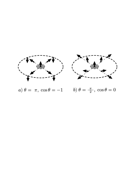
FIG. 1.: The profile of the non-singular vortex; a) The case of $\theta(\infty)=\pi$ and b) The case of $\theta(\infty)={\pi\over 2}$.

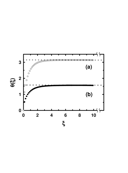
FIG. 2.: The profile of the function $\theta(\xi)$ for two cases of boundary conditions: (a) $\theta(\infty)=\pi$ and (b) $\theta(\infty)={\pi\over 2}$.

REFERENCES

- [1] R. Y. Chiao, E. Gamire, and C. H. Townes, Phys. Rev. Lett. 13, 479 (1964).
- [2] A. W. Snyder, L. Polarian, and D.J. Mitchell, Opt. Lett. 17, 789 (1992).
- [3] G. A. Swartzlander, Jr. and C. T. Law, Phys. Rev. Lett. 69, 2503 (1992).
- [4] D. Rozas, Z.S. Sacks and G.A. Swartzlander, Jr., Phys. Rev. Lett. 79, 3399 (1997).
- [5] A. W. Snyder, S. J. Hewlett and D. J. Mitchell, Phys. Rev. Lett.72 1012(1994).
- [6] M. Born and E. Wolf, Principle of Optics (Pergamon, Oxford, 1975).
- [7] L. Landau and E. Lifschitz, Electrodynamics in Continuous Media, chapter 11, Course of Theoretical Physics Vol.8 (Pergamon Oxford, 1968).
- [8] H. Kuratsuji and S. Kakigi, Phys. Rev. Lett. 80, 1888 (1998) and references cited therein.
- [9] We here discard the term that is proportional to , since is a slowly varying function. See [7].
- [10] See S.A.Akhmanov, Physical Optics, Chapter 14 (Clarendon press, Oxford 1997), where the quasi-otical approximation is used ; .
- [11] C.Brosseau, Fundamental of Polarized Light: A Statistical Optics Approach, Chapter 3, (John Wiley, New York, 1998).
- [12] H. Ono and H. Kuratsuji, Phys. Lett. 186A, 255(1994), H. Kuratsuji and H. Yabu, J. Phys. A29, 6505(1996).
- [13] We note that in (23) does not depend on , because the integrand of is a function of , and with a change of the variable , becomes independent from .
- [14] e.g. H. Lamb, Hydrodymanics, (Cambridge University Press, 1932) p248.