Quantum phase transitions in electronic systems

Abstract

Quantum phase transitions occur at zero temperature when some non-thermal control-parameter like pressure or chemical composition is changed. They are driven by quantum rather than thermal fluctuations. In this review we first give a pedagogical introduction to quantum phase transitions and quantum critical behavior emphasizing similarities with and differences to classical thermal phase transitions. We then illustrate the general concepts by discussing a few examples of quantum phase transitions occurring in electronic systems. The ferromagnetic transition of itinerant electrons shows a very rich behavior since the magnetization couples to additional electronic soft modes which generates an effective long-range interaction between the spin fluctuations. We then consider the influence of rare regions on quantum phase transitions in systems with quenched disorder, taking the antiferromagnetic transitions of itinerant electrons as a primary example. Finally we discuss some aspects of the metal-insulator transition in the presence of quenched disorder and interactions.

1 Classical and quantum phase transitions

1.1 Introduction

Phase transitions have played, and continue to play, an essential role in shaping the world. The large scale structure of the universe is the result of a sequence of phase transitions during the very early stages of its development. Later, phase transitions accompanied the formation of galaxies, stars and planets. Even our everyday life is unimaginable without the never ending transformations of water between ice, liquid and vapor. Understanding phase transitions is a thus a prime endeavor of physics.

Under normal conditions the phase transitions of water are so-called first-order transitions. They involve latent heat, i.e., a finite amount of heat is released while the material is cooled through an infinitesimally small temperature interval around the transition temperature. Phase transitions that do not involve latent heat, the so-called continuous transitions, are particularly interesting since the typical length and time scales of fluctuations of, e.g., the density, diverge when approaching the transition point. These divergences and the resulting singularities of physical observables are called the critical behavior. Understanding critical behavior has been a great challenge for theoretical physics. More than a century has gone by from the first discoveries until a consistent picture emerged. However, the theoretical concepts established during this development, viz., scaling and the renormalization group, now belong to the central paradigms of modern physics.

The phase transitions we encounter in everyday life occur at finite temperature. These so-called thermal or classical phase transitions are driven by thermal fluctuations. In recent years a different class of phase transitions, the so-called quantum phase transitions, has started to attract a lot of attention. Quantum phase transitions occur at zero temperature when some non-thermal control parameter is changed. They are driven by quantum rather than thermal fluctuations. Quantum phase transitions in electronic systems have gained particular attention since some of the most exciting discoveries in contemporary condensed matter physics, such as the localization problem, various magnetic phenomena, integer and fractional quantum Hall effects, and high-temperature superconductivity are often attributed to quantum critical points.

The purpose of this review is twofold. The first section gives a pedagogical introduction to the field of quantum phase transitions with a particular emphasis on the similarities with and the differences to classical thermal phase transitions. After briefly sketching the historical development the basic concepts of continuous phase transitions and critical behavior are summarized. We then consider the question ’How important is quantum mechanics for the physics of phase transitions?’ which leads directly to the distinction between classical thermal and quantum phase transitions. In the following sections these ideas are illustrated by discussing a number of examples of quantum phase transitions occurring in electronic systems. Specifically, in Sec. 2 a toy model for a quantum phase transition is considered, the so-called quantum spherical model. It can be solved exactly, providing an easily accessible example of a quantum phase transition. Sec. 3 contains a discussion of the ferromagnetic quantum phase transition of itinerant electrons. It is demonstrated that the coupling of the magnetization to additional soft modes in the zero-temperature electron system changes the properties of the transition profoundly. The influence of disorder on quantum phase transitions is studied in Sec. 4 paying particular attention to rare disorder fluctuations. It is shown that they can change the universality class of the transition or even destroy the conventional critical behavior. In Sec. 5 we discuss some aspects of the metal-insulator transition of disordered interacting electrons. On the one hand we consider the influence of local moments on the transition by incorporating them into a transport theory. On the other hand we study the transition by means of large-scale numerical simulations. To do this, an efficient numerical method is developed, called the Hartree-Fock based diagonalization. It is shown that electron-electron interactions can lead to a considerable enhancement of transport in the strongly localized regime. Finally, Sec. 6 is devoted to a short summary and outlook.

1.2 From critical opalescence to quantum criticality

In 1869 Andrews [1] discovered a very special point in the phase diagram of carbon dioxide. At a temperature of about 31 ^∘C and 73 atmospheres pressure the properties of the liquid and the vapor phases became indistinguishable. In the neighborhood of this point carbon dioxide strongly scattered light. Andrews called this point the critical point and the strong light scattering the critical opalescence. Four years later van der Waals [2] presented his doctoral thesis ’On the continuity of the liquid and gaseous states’ which contained one of the first theoretical explanations of critical phenomena based on the now famous van der Waals equation of state. It provides the prototype of a mean-field description of a phase transition by assuming that the individual interactions between the molecules are replaced by an interaction with a hypothetic global mean field. In the subsequent years similar behavior was found for many other materials. In particular, in 1895 Pierre Curie [3] noticed that ferromagnetic iron also shows such a critical point which today is called the Curie point. It is located at zero magnetic field and a temperature of about 770 ^∘C, the highest temperature for which a permanent magnetization can exist in zero field. At this temperature phases differing by the direction of the magnetization become obviously indistinguishable. Again it was only a few years later when Weiss [4] proposed the molecular-field theory of ferromagnetism which qualitatively explained the experiments. Like the van der Waals theory of the liquid-gas transition the molecular-field theory of ferromagnetism is based on the existence of a hypothetic molecular (mean) field. The so-called classic era of critical phenomena culminated in the Landau theory of phase transitions [5]. Landau gave some very powerful and general arguments based on symmetry which suggested that mean-field theory is essentially exact. While we know today that this is not the case, Landau theory is still an invaluable starting point for the investigation of critical phenomena.

The modern era of critical phenomena started when it was realized that there was a deep problem connected with the values of the critical exponents which describe how physical quantities vary close to the critical point. In 1945 Guggenheim [6] realized that the coexistence curve of the gas–fluid phase transition is not parabolic, as predicted by van der Waals’ mean-field theory. At about the same time Onsager [7] exactly solved the two-dimensional Ising model showing rigorously that in this system the critical behavior is different from the predictions of mean-field theory. After these observations it took about twenty years until a solution of the ’exponent puzzle’ was approached. In 1965 Widom [8] formulated the scaling hypothesis according to which the singular part of the free energy is a generalized homogeneous function of the parameters. A year later, Kadanoff [9] proposed a simple heuristic explanation of scaling based on the argument that at criticality the system essentially ’looks the same on all length scales’. The breakthrough came with a series of seminal papers by Wilson [10] in 1971. He formalized Kadanoff’s heuristic arguments and developed the renormalization group. For these discoveries, Wilson won the 1982 physics Nobel price. The development of the renormalization group initiated an avalanche of activity in the field which still continues.

Today, thermal equilibrium phase transitions are well understood in principle, even if new interesting transitions, e.g., in soft condensed matter systems, continue to be found. In recent years the scientific interest has shifted towards new fields. One of these fields are phase transitions in non-equilibrium systems. They occur, e.g., in systems approaching equilibrium after a non-infinitesimal perturbation or in systems driven by external fields or non-thermal noise to a non-equilibrium (steady) state. Examples are provided by growing surfaces, chemical reaction-diffusion systems, or biological systems (see, e.g., Refs. [11, 12, 13]). Non-equilibrium phase transitions are characterized by singularities in the stationary or dynamic properties of the non-equilibrium states rather than by thermodynamic singularities.

Another very active avenue of research are quantum phase transitions which are the topic of this review. The investigation of quantum phase transitions was pioneered by Hertz [14] who built on earlier work by Suzuki [15] and Beal-Monod [16]. He developed a renormalization group method for magnetic transitions of itinerant electrons which was a direct generalization of Wilson’s approach to classical transitions. He found that the ferromagnetic transition is mean-field like in all dimensions $d>1$. While Hertz’ general scaling scenario at a quantum critical point is valid, his specific predictions for the ferromagnetic quantum phase transition are incorrect, as will be explained in Sec. 3.

In recent years quantum phase transitions in electronic systems have attracted considerable attention from theory as well from experiment. Among the transitions investigated in detail are the ferromagnetic transition of itinerant electrons, the antiferromagnetic transition associated with high-temperature superconductivity, various magnetic transitions in the heavy fermion compounds, metal-insulator transitions, superconductor-insulator transitions, and the plateau transition in quantum Hall systems. This list is certainly incomplete and new transitions continue to be found. For reviews on some of these transitions see, e.g., Refs. [17, 18, 19, 20, 21, 22]. There is also a very recent text book on quantum phase transitions by Sachdev [23].

1.3 Basic concepts of phase transitions and critical behavior

Since the discoveries of scaling and the renormalization group a number of excellent text books on phase transitions and critical behavior have appeared (e.g., those by Ma [24] or Goldenfeld [25]). Therefore, in this section we only briefly collect the basic concepts which are necessary for the later discussion.

A continuous phase transition can usually be characterized by an order parameter, a concept first introduced by Landau. An order parameter is a thermodynamic quantity that is zero in one phase (the disordered) and non-zero and non-unique in the other (the ordered) phase. Very often the choice of an order parameter for a particular transition is obvious as, e.g., for the ferromagnetic transition where the total magnetization is an order parameter. Sometimes, however, finding an appropriate order parameter is a complicated problem by itself, e.g., for the disorder-driven localization-delocalization transition of non-interacting electrons.

While the thermodynamic average of the order parameter is zero in the disordered phase, its fluctuations are non-zero. If the phase transition point, i.e., the critical point, is approached the spatial correlations of the order parameter fluctuations become long-ranged. Close to the critical point their typical length scale, the correlation length $\xi$, diverges as

$$\xi\propto t^{-\nu}$$ (1)

where $\nu$ is the correlation length critical exponent and $t$ is some dimensionless distance from the critical point. It can be defined as $t=|T-T_{c}|/T_{c}$ if the transition occurs at a non-zero temperature $T_{c}$. In addition to the long-range correlations in space there are analogous long-range correlations of the order parameter fluctuations in time. The typical time scale for a decay of the fluctuations is the correlation (or equilibration) time $\tau_{c}$. As the critical point is approached the correlation time diverges as

$$\tau_{c}\propto\xi^{z}\propto t^{-\nu z}$$ (2)

where $z$ is the dynamical critical exponent. Close to the critical point there is no characteristic length scale other than $\xi$ and no characteristic time scale other than $\tau_{c}$. As already noted by Kadanoff [9], this is the physics behind Widom’s scaling hypothesis, which we will now discuss.

Let us consider a classical system, characterized by its Hamiltonian

$$H(p_{i},q_{i})=H_{kin}(p_{i})+H_{pot}(q_{i})$$ (3)

where $q_{i}$ and $p_{i}$ are the generalized coordinates and momenta, and $H_{kin}$ and $H_{pot}$ are the kinetic and potential energies, respectively. In such a system ’statics and dynamics decouple’, i.e., the momentum and position sums in the partition function

$$Z=\int\prod dp_{i}e^{-H_{kin}/k_{B}T}~{}\int\prod dq_{i}e^{-H_{pot}/k_{B}T}=Z_{kin}Z_{pot}$$ (4)

are completely independent from each other. The kinetic contribution to the free energy density $f=-(k_{B}T/V)\log Z$ will usually not display any singularities, since it derives from the product of simple Gaussian integrals. Therefore one can study the critical behavior using effective time-independent theories like the Landau-Ginzburg-Wilson theory. In this type of theories the free energy is expressed as a functional of the order parameter $M({\bf r})$ only. All other degrees of freedom have been integrated out in the derivation of the theory starting from a microscopic Hamiltonian. In its simplest form [5, 10, 26] valid, e.g., for an Ising ferromagnet, the Landau-Ginzburg-Wilson functional $\Phi[M]$ reads

$$\Phi[M] = \int d^{d}r~{}M({\bf r})\left(-\frac{\partial^{2}}{\partial{\bf r}^{2}}+t\right)M({\bf r})+u\int d^{d}r~{}M^{4}({\bf r})-B\int d^{d}r~{}M({\bf r}),$$

$$Z = \int D[M]e^{-\Phi[M]}\quad,$$ (5)

where $B$ is the field conjugate to the order parameter (the magnetic field in case of a ferromagnet).

Since close to the critical point the correlation length is the only relevant length scale, the physical properties must be unchanged, if we rescale all lengths in the system by a common factor $b$, and at the same time adjust the external parameters in such a way that the correlation length retains its old value. This gives rise to the homogeneity relation for the free energy density,

$$f(t,B)=b^{-d}f(t\,b^{1/\nu},B\,b^{y_{B}}).$$ (6)

Here $y_{B}$ is another critical exponent. The scale factor $b$ is an arbitrary positive number. Analogous homogeneity relations for other thermodynamic quantities can be obtained by differentiating $f$. The homogeneity law (6) was first obtained phenomenologically by Widom [8]. Within the framework of the renormalization group theory it can be derived from first principles.

In addition to the critical exponents $\nu,~{}y_{B}$ and $z$ defined above, a number of other exponents is in common use. They describe the dependence of the order parameter and its correlations on the distance from the critical point and on the field conjugate to the order parameter. The definitions of the most commonly used critical exponents are summarized in Table 1.

Table 1: Definitions of the commonly used critical exponents in the ’magnetic language’, i.e., the order parameter is the magnetization $m=\langle M\rangle$, and the conjugate field is a magnetic field $B$. $t$ denotes the distance from the critical point and $d$ is the space dimensionality. (The exponent $y_{B}$ defined in (6) is related to $\delta$ by $y_{B}=d\,\delta/(1+\delta)$.)

	exponent	definition	conditions
specific heat	$\alpha$	$c\propto|t|^{-\alpha}$	$t\to 0,B=0$
order parameter	$\beta$	$m\propto(-t)^{\beta}$	$t\to 0$ from below, $B=0$
susceptibility	$\gamma$	$\chi\propto|t|^{-\gamma}$	$t\to 0,B=0$
critical isotherm	$\delta$	$B\propto|m|^{\delta}{\rm sign}(m)$	$B\to 0,t=0$
correlation length	$\nu$	$\xi\propto|t|^{-\nu}$	$t\to 0,B=0$
correlation function	$\eta$	$G(r)\propto|r|^{-d+2-\eta}$	$t=0,B=0$
dynamical	$z$	$\tau_{c}\propto\xi^{z}$	$t\to 0,B=0$

Note that not all the exponents defined in Table 1 are independent from each other. The four thermodynamic exponents $\alpha,\beta,\gamma,\delta$ can all be obtained from the free energy (6) which contains only two independent exponents. They are therefore connected by the so-called scaling relations

$$2-\alpha = 2\beta+\gamma~{},$$ (7)

$$2-\alpha = \beta(\delta+1)~{}.$$ (8)

Analogously, the exponents of the correlation length and correlation function are connected by two so-called hyperscaling relations

$$2-\alpha = d\,\nu~{},$$ (9)

$$\gamma = (2-\eta)\nu~{}.$$ (10)

Since statics and dynamics decouple in classical statistics the dynamical exponent $z$ is completely independent from all the others.

The critical behavior at a particular phase transition is completely characterized by the set of critical exponents. One of the most remarkable features of continuous phase transitions is universality, i.e., the fact that the critical exponents are the same for entire classes of phase transitions which may occur in very different physical systems. These classes, the so-called universality classes, are determined only by the symmetries of the Hamiltonian and the spatial dimensionality of the system. This implies that the critical exponents of a phase transition occurring in nature can be determined exactly (at least in principle) by investigating any simplistic model system belonging to the same universality class, a fact that makes the field very attractive for theoretical physicists. The mechanism behind universality is again the divergence of the correlation length. Close to the critical point the system effectively averages over large volumes rendering the microscopic details of the Hamiltonian unimportant.

The critical behavior at a particular transition is crucially determined by the relevance or irrelevance of order parameter fluctuations. It turns out that fluctuations become increasingly important if the spatial dimensionality of the system is reduced. Above a certain dimension, called the upper critical dimension $d_{c}^{+}$, fluctuations are irrelevant, and the critical behavior is identical to that predicted by mean-field theory (for systems with short-range interactions and a scalar or vector order parameter $d_{c}^{+}=4$). Between $d_{c}^{+}$ and a second special dimension, called the lower critical dimension $d_{c}^{-}$, a phase transition still exists but the critical behavior is different from mean-field theory. Below $d_{c}^{-}$ fluctuations become so strong that they completely suppress the ordered phase.

1.4 How important is quantum mechanics?

The question of to what extent quantum mechanics is important for understanding a continuous phase transition is a multi-layered question. One may ask, e.g., whether quantum mechanics is necessary to explain the existence and the properties of the ordered phase. This question can only be decided on a case-by-case basis, and very often quantum mechanics is essential as, e.g., for superconductors. A different question to ask would be how important quantum mechanics is for the asymptotic behavior close to the critical point and thus for the determination of the universality class the transition belongs to.

It turns out that the latter question has a remarkably clear and simple answer: Quantum mechanics does not play any role for the critical behavior if the transition occurs at a finite temperature. It does play a role, however, at zero temperature. In the following we will first give a simple argument explaining these facts. To do so it is useful to distinguish fluctuations with predominantly thermal and quantum character depending on whether their thermal energy $k_{B}T$ is larger or smaller than the quantum energy scale $\hbar\omega_{c}$. We have seen in the preceeding section that the typical time scale $\tau_{c}$ of the fluctuations diverges as a continuous transition is approached. Correspondingly, the typical frequency scale $\omega_{c}$ goes to zero and with it the typical energy scale

$$\hbar\omega_{c}\propto|t|^{\nu z}~{}.$$ (11)

Quantum fluctuations will be important as long as this typical energy scale is larger than the thermal energy $k_{B}T$. If the transition occurs at some finite temperature $T_{c}$ quantum mechanics will thus become unimportant for $|t|<t_{x}$ with the crossover distance $t_{x}$ given by

$$t_{x}\propto T_{c}^{1/\nu z}~{}.$$ (12)

We thus find that the critical behavior asymptotically close to the transition is entirely classical if the transition temperature $T_{c}$ is nonzero. This justifies to call all finite-temperature phase transitions classical transitions, even if the properties of the ordered state are completely determined by quantum mechanics as is the case, e.g., for the superconducting phase transition of, say, mercury at $T_{c}=4.2$ K. In these cases quantum fluctuations are obviously important on microscopic scales, while classical thermal fluctuations dominate on the macroscopic scales that control the critical behavior. If, however, the transition occurs at zero temperature as a function of a non-thermal parameter like the pressure $p$, the crossover distance $t_{x}=0$. (Note that at zero temperature the distance $t$ from the critical point cannot be defined via the reduced temperature. Instead, one can define $t=|p-p_{c}|/p_{c}$.) Thus, at zero temperature the condition $|t|<t_{x}$ is never fulfilled, and quantum mechanics will be important for the critical behavior. Consequently, transitions at zero temperature are called quantum phase transitions.

Let us now generalize the homogeneity law (6) to the case of a quantum phase transition. We consider a system characterized by a Hamiltonian $H$. In a quantum problem kinetic and potential part of $H$ in general do not commute. In contrast to the classical partition function (4) the quantum mechanical partition function does not factorize, i.e., ’statics and dynamics are always coupled’. The canonical density operator $e^{-H/k_{B}T}$ looks exactly like a time evolution operator in imaginary time $\tau$ if one identifies

$$1/k_{B}T=\tau=-i\Theta/\hbar$$ (13)

where $\Theta$ denotes the real time. This naturally leads to the introduction of an imaginary time direction into the system. An order parameter field theory analogous to the classical Landau-Ginzburg-Wilson theory (5) therefore needs to be formulated in terms of space and time dependent fields. The simplest example of a quantum Landau-Ginzburg-Wilson functional, valid for, e.g., an Ising model in a transverse field, reads

$$\Phi[M] = \int_{0}^{1/k_{B}T}d\tau\int d^{d}r~{}M({\bf r},\tau)\left(-\frac{\partial^{2}}{\partial{\bf r}^{2}}-\frac{\partial^{2}}{\partial\tau^{2}}+t\right)M({\bf r},\tau)~{}+$$ (14)

$$+ u\int_{0}^{1/k_{B}T}d\tau\int d^{d}r~{}M^{4}({\bf r},\tau)~{}-~{}B\int_{0}^{1/k_{B}T}d\tau\int d^{d}r~{}M({\bf r},\tau)~{}.$$

Let us note that the coupling of statics and dynamics in quantum statistical dynamics also leads to the fact that the universality classes for quantum phase transitions are smaller than those for classical transitions. Systems which belong to the same classical universality class may display different quantum critical behavior, if their dynamics differ.

The classical homogeneity law (6) for the free energy density can now easily be adopted to the case of a quantum phase transition. At zero temperature the imaginary time acts similarly to an additional spatial dimension since the extension of the system in this direction is infinite. According to (2), time scales like the $z$th power of a length. (In the simple example (14) space and time enter the theory symmetrically leading to $z=1$.) Therefore, the homogeneity law for the free energy density at zero temperature reads

$$f(t,B)=b^{-(d+z)}f(t\,b^{1/\nu},B\,b^{y_{B}})~{}.$$ (15)

Comparing (15) and (6) directly shows that a quantum phase transition in $d$ dimensions is equivalent to a classical transition in $d+z$ spatial dimensions. Thus, for a quantum phase transition the upper critical dimension, above which mean-field critical behavior becomes exact, is reduced by $z$ compared to the corresponding classical transition.

Now the attentive reader may ask: Why are quantum phase transitions more than an academic problem? Any experiment is done at a non-zero temperature where, as we have explained above, the asymptotic critical behavior is classical. The answer is again provided by the crossover condition (12): If the transition temperature $T_{c}$ is very small quantum fluctuations will remain important down to very small $t$, i.e., very close to the transition. At a more technical level, the behavior at small but non-zero temperatures is determined by the crossover between two types of critical behavior, viz. quantum critical behavior at $T=0$ and classical critical behavior at non-zero temperatures. Since the ’extension of the system in imaginary time direction’ is given by the inverse temperature $1/k_{B}T$ the corresponding crossover scaling is equivalent to finite size scaling in imaginary time direction. The crossover from quantum to classical behavior will occur when the correlation time $\tau_{c}$ reaches $1/k_{B}T$ which is equivalent to the condition (12). By adding the temperature as an explicit parameter and taking into account that in imaginary-time formalism it scales like an inverse time (13), we can generalize the quantum homogeneity law (15) to finite temperatures,

$$f(t,B,T)=b^{-(d+z)}f(t\,b^{1/\nu},B\,b^{y_{B}},T\,b^{z})~{}.$$ (16)

The resulting phase diagram close to a quantum critical points will be of one of two qualitative different types. The first type describes situations where an ordered phase exists at finite temperature. These phase diagrams are illustrated in Fig. 1.

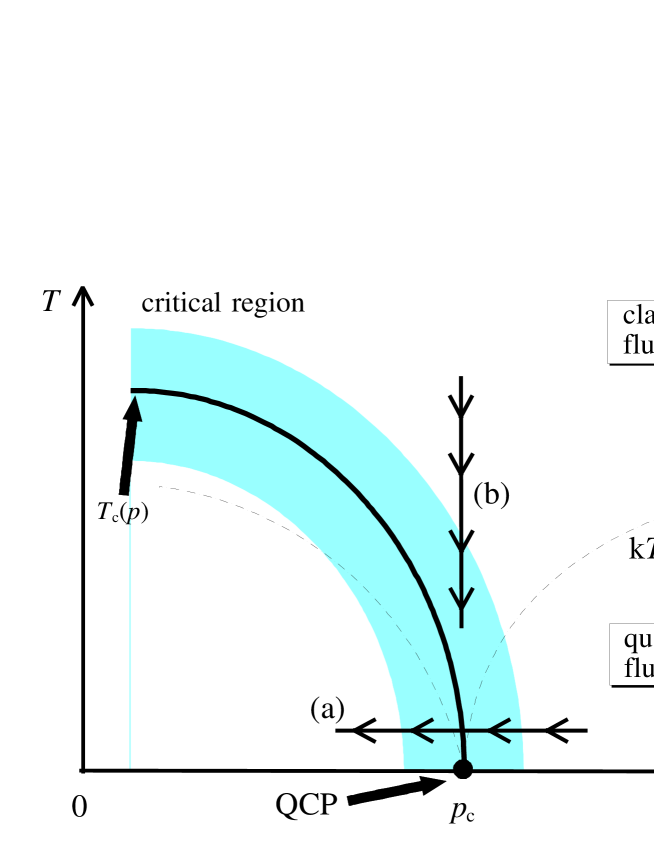
Figure 1: Schematic phase diagram in the vicinity of a quantum critical point (QCP). The solid line marks the boundary between ordered and disordered phase. The dashed lines indicate the crossover between predominantly quantum or classical character of the fluctuations, and the shaded area denotes the critical region where the leading critical singularities can be observed. Paths (a) and (b) are discussed in the text.

Here $p$ stands for the (non-thermal) parameter which tunes the quantum phase transition. According to (12) the vicinity of the quantum critical point can be divided into regions with predominantly classical or quantum fluctuations. The boundary, marked by the dashed lines in Fig. 1, is not sharp but rather a smooth crossover line. At sufficiently low temperatures these crossover lines are inside the critical region (i.e., the region where the leading critical power laws can be observed). An experiment performed along path (a) will therefore observe a crossover from quantum critical behavior away from the transition to classical critical behavior asymptotically close to it. At very low temperatures the classical region may become so narrow that it is actually unobservable in an experiment.

In addition to the critical behavior at very low temperatures, the quantum critical point also controls the behavior in the so-called quantum critical region [27]. This region is located at the critical $p$ but, somewhat counter-intuitively, at comparatively high temperatures (where the character of the fluctuations is classical). In this region the system ’looks critical’ with respect to $p$ but is driven away from criticality by the temperature (i.e., the critical singularities are exclusively protected by $T$). An experiment carried out along path (b) will therefore observe the temperature scaling at the quantum critical point.

The second type of phase diagram occurs if an ordered phase exists at zero temperature only (as is the case for two-dimensional quantum antiferromagnets). In this case there will be no true phase transition in any experiment. However, the system will display quantum critical behavior in the above-mentioned quantum critical region close to the critical $p$.

2 Quantum spherical model

2.1 Classical spherical model

In the process of understanding a novel physical problem it is often very useful to consider a simple model which displays the phenomena in question in their most basic form. In the field of classical equilibrium critical phenomena such a model is the so-called classical spherical model which is one of the very few models in statistical physics that can be solved exactly but show non-trivial (i.e., non mean-field) critical behavior. The spherical model was conceived by Kac in 1947 in an attempt to simplify the Ising model. The basic idea was to replace the discrete Ising spins having only the two possible values $S_{i}=\pm 1$ by continuous real variables between $-\infty$ and $\infty$ so that the multiple sum in the partition function of the Ising model is replaced by a multiple integral which should be easier to perform. However, the multiple integral turned out to be not at all simple, and for a time it looked as if the spherical model was actually harder to solve than the corresponding Ising model. Eventually Berlin and Kac [28] solved the spherical model by using the method of steepest descent to perform the integrals over the spin variables. Stanley [29] showed that the spherical model, though created to be a simplification of the Ising model, is equivalent to the $n\to\infty$ limit of the classical $n$-vector model. Therefore, it can be used as the starting point for a $1/n$-expansion of the critical behavior.

In the following years the classical spherical model was solved exactly not only for nearest neighbor ferromagnetic interactions but also for long-range power-law interactions [30], random interactions [31, 32], systems in random magnetic fields [33, 34], and disordered electronic systems with localized states [35]. Moreover, the model has been used as a test case for the finite-size scaling hypothesis [36, 37]. Reviews on the classical spherical model were given by Joyce [38] and Khorunzhy et al. [39].

Because the classical spherical model possesses such a wide variety of applications in the field of classical critical phenomena, it seems natural to look for a quantum version of the model in order to obtain a toy model for quantum critical behavior. Actually, the history of quantum spherical models dates back at least as far as the history of quantum critical behavior. In 1972 Obermair [40] suggested a canonical quantization scheme for a dynamical spherical model. However, this and later studies focused on the classical finite temperature critical behavior of the quantum model and did not consider the properties of the zero temperature quantum phase transition.

2.2 Quantization of the spherical model

The classical spherical model consists of $N$ real variables $S_{i}\in(-\infty,\infty)$ that interact with an external field $h_{i}$ and with each other via a pair potential $U_{ij}$. The Hamiltonian is given by

$$H_{cl}=\frac{1}{2}\sum_{i,j}U_{ij}S_{i}S_{j}+\sum_{i}h_{i}S_{i}~{}.$$ (17)

In order to make the model well-defined at low temperatures, i.e., in order to prevent a divergence of $S_{i}$ in the ordered phase, the values of $S_{i}$ are subject to an additional constraint, the so-called spherical constraint. Two versions of the constraint have been used in the literature, the strict and the mean constraints, defined by

$$\sum_{i}S_{i}^{2} = N,$$ (18)

$$\sum_{i}\langle S_{i}^{2}\rangle = N,$$ (19)

respectively. Here $\langle\ldots\rangle$ is the thermodynamic average. Both constraints have been shown to give rise to the same thermodynamic behavior while other quantities like correlation functions differ. In the following we restrict ourselves to the mean spherical constraint which is easier to implement in the quantum case. The Hamiltonian (17) has no internal dynamics. According to the factorization (4) it can be interpreted as being only the configurational part of a more complicated problem. Therefore, the construction of the quantum model consists of two steps: First we have to add an appropriate kinetic energy to the Hamiltonian which defines a dynamical spherical model which can be quantized in a second step.

In order to construct the kinetic energy term we define canonically conjugate momentum variables $P_{i}$ which fulfill the Poisson bracket relations $\{S_{i},P_{j}\}=\delta_{ij}$. The simplest choice of a kinetic energy term is then the one of Obermair [40], $H_{kin}=\frac{g}{2}\sum_{i}P_{i}^{2}$, where $g$ can be interpreted as inverse mass. In this case, the complete Hamiltonian of the dynamical spherical model

$$H=H_{kin}+H_{cl}=\frac{g}{2}\sum_{i}P_{i}^{2}+\frac{1}{2}\sum_{i,j}U_{ij}S_{i}S_{j}+\sum_{i}h_{i}S_{i}+\mu\left(\sum_{i}S_{i}^{2}-N\right)$$ (20)

is that of a system of coupled harmonic oscillators. Here we have also added a source term for the mean spherical constraint (19). (The value of $\mu$ has to be determined self-consistently so that (19) is fulfilled.)

In order to quantize the dynamical spherical model (20) we use the usual canonical quantization scheme: The variables $S_{i}$ and $P_{i}$ are reinterpreted as operators. The Poisson bracket relations are replaced by the corresponding canonical commutation relations

$$[S_{i},S_{j}]=0,~{}[P_{i},P_{j}]=0,~{}{\rm and}~{}[S_{i},P_{j}]=i\hbar\delta_{ij}~{}.$$ (21)

Equations (19), (20), and (21) completely define the quantum spherical model. At large $T$ or $g$ the model is in its disordered phase $\langle S_{i}\rangle=0$. The transition to an ordered state can be triggered by lowering $g$ and/or $T$.

It must be emphasized that this model does not mimic (or even describe) Heisenberg-Dirac spins. Instead it is equivalent to the $n\to\infty$ limit of a quantum rotor model which can be seen as a generalization of an Ising model in a transverse field. Of course, the choices of the kinetic energy and quantization scheme are not unique. In agreement with the general discussion in Sec. 1.4 different choices will lead to different critical behavior at the quantum phase transition, while the classical critical behavior is the same for all these models. An example of a different quantization of the spherical model was given by Nieuwenhuizen [41]. It leads to a dynamical behavior that more closely resembles that of Heisenberg-Dirac spins than our choice. For a more detailed discussion of these questions see also Ref. [42].

2.3 Quantum phase transitions

The quantum spherical model defined in eqs. (19), (20), and (21) can be solved exactly since it is equivalent to a system of coupled harmonic oscillators. This was done in Ref. [42] for a model with arbitrary translationally invariant interactions (long-range as well as short-range) in a spatially homogeneous external field. The resulting free energy reads

$$f=-\frac{k_{B}T}{N}\ln Z=-\mu-\frac{h^{2}}{4\mu}+\frac{k_{B}T}{N}\sum_{k}\ln\left(2\sinh\frac{\omega(k)}{2k_{B}T}\right)~{},$$ (22)

with $\omega(k)$ given by $\omega^{2}=2g[\mu+U(k)/2]$, where $U(k)$ is the Fourier transform of the interaction $U_{ij}$. The spherical constraint which determines $\mu$ is given by

$$0=\frac{\partial f}{\partial\mu}=-1+\frac{h^{2}}{4\mu^{2}}+\frac{1}{N}\sum_{k}\frac{g}{2\omega(k)}\coth\frac{\omega(k)}{2k_{B}T}~{}.$$ (23)

As usual in spherical models the critical behavior is determined by the properties of the solutions of (23) for small $\mu$. At any finite temperature the $\coth$-term can be expanded giving the same leading long-wavelength and low frequency terms as in the classical spherical model (17). As expected, the resulting critical behavior at finite temperatures is therefore that of the classical spherical model.

At zero temperature, the $\coth$-term in (23) is identical to one. Thus, the leading long-wavelength and low frequency terms are different from the classical case. This gives rise to the quantum critical behavior being different from the classical one. If the interaction $U_{ij}$ in the Hamiltonian is short ranged, the dynamical exponent turns out to be $z=1$. For a power-law interaction, parameterized by the singularity of the Fourier transform of the interaction, $U_{k}\propto|k|^{x}$ for $k\to 0$, we obtain $z=x/2$. In both cases the quantum critical behavior of the $d$-dimensional quantum spherical model is the same as the classical critical behavior of a corresponding $d+z$-dimensional model. The critical exponents for the quantum and classical phase transitions are summarized in Table 2.

Table 2: Critical exponents at the quantum and classical phase transitions of the quantum spherical model as functions of the dimensionality $d$ and the exponent $x$ which characterizes the long-wavelength behavior of the interaction $U(k)\sim|k|^{x}$ (short-range interactions correspond to $x=2$).

	Quantum transition	Classical transition	Both
exponent	$d<d_{c}^{+}=3x/2$	$d<d_{c}^{+}=2x$	$d>d_{c}^{+}$
$\alpha$	$(2d-3x)/(2d-x)$	$(d-2x)/(d-x)$	0
$\beta$	1/2	1/2	1/2
$\gamma$	$2x/(2d-x)$	$x/(d-x)$	1
$\delta$	$(2d+3x)/(2d-x)$	$(d+x)/(d-x)$	3
$\nu$	$2/(2d-x)$	$1/(d-x)$	$1/x$
$\eta$	$2-x$	$2-x$	$2-x$
$z$	$x/2$	$x/2$	$x/2$

In order to describe the crossover between the quantum and classical critical behaviors the crossover scaling form of the equation of state was derived. This is only possible below the upper critical dimension. Above, crossover scaling breaks down. This is analogous to the breakdown of finite-size scaling in the spherical model above the upper critical dimension. It can be attributed to a dangerous irrelevant variable.

In Ref. [43] the influence of a quenched random field on the quantum phase transition was considered. The quantum spherical model can be solved exactly even in the presence of a random field without the necessity to use the replica trick. It was found that the quantum critical behavior is dominated by the static random field fluctuations rather than by the quantum fluctuations. Since the random field fluctuations are identical at zero and finite temperatures it follows that in the presence of a random field quantum and classical critical behavior are identical.

3 Ferromagnetic quantum phase transition of itinerant electrons

3.1 Itinerant ferromagnets

In the normal metallic state the electrons form a Fermi liquid, a concept introduced by Landau [44, 45]. In this state the excitation spectrum is very similar to that of a non-interacting Fermi gas. The basic excitations are weakly interacting fermionic quasiparticles which behave like normal electrons but have renormalized parameters like an effective mass. However, at low temperatures the Fermi liquid is potentially unstable against sufficiently strong interactions, and some type of a symmetry-broken state may form. This low-temperature phase may be a superconductor, a charge density wave, or a magnetic phase, e.g., a ferromagnet, an anti-ferromagnet, or a spin glass, to name a few possibilities. In general, it will depend on the microscopic parameters of the material under consideration what the nature of the low-temperature phase and, specifically, of the ground state will be. Upon changing these microscopic parameters at zero temperature, e.g., by applying pressure or an external field or by changing chemical composition, the nature of the ground state may change, i.e., the system may undergo a quantum phase transition.

In this Section we will discuss a particular example of such a quantum phase transition, viz. the ferromagnetic quantum phase transition of itinerant electrons. Most of the Section will be devoted to clean itinerant electrons but we will also briefly consider the influence of disorder on the ferromagnetic transition.

The experimentally best studied example of a ferromagnetic quantum phase transition of itinerant electrons is probably provided by the pressure-tuned transition in MnSi [46, 47]. MnSi belongs to the class of so-called nearly or weakly ferromagnetic materials. This group of metals, consisting of transition metals and their compounds such as ZrZn₂, TiBe₂, Ni₃Al, and YCo₂ in addition to MnSi are characterized by strongly enhanced spin fluctuations. Thus, their ground state is close to a ferromagnetic instability which makes them good candidates for actually reaching the ferromagnetic quantum phase transition in experiment by changing the chemical composition or applying pressure.

At ambient pressure MnSi is paramagnetic for temperatures larger than $T_{c}=30$ K. Below $T_{c}$ it orders magnetically. The order is, however, not exactly ferromagnetic but a long-wavelength (190 Å) helical spin spiral along the (111) direction of the crystal. The ordering wavelength depends only weakly on the temperature, but a homogeneous magnetic field of about 0.6 T suppresses the spiral and leads to ferromagnetic order. One of the most remarkable findings about the magnetic phase transition in MnSi is that it changes from continuous to first order with decreasing temperature as is shown in Fig. 2.

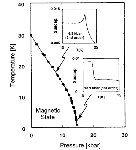
Figure 2: Phase diagram of MnSi. The insets show the behavior of the susceptibility close to the transition. (after Ref. [46])

Specifically, in an experiment carried out at low pressure (corresponding to a comparatively high transition temperature) the susceptibility shows a pronounced maximum at the transition, reminiscent of the singularity expected from a continuous phase transition. In contrast, in an experiment at a pressure very close to (but still smaller than) the critical pressure the susceptibility does not show any sign of a divergence at the phase transition. Instead, it displays a finite step suggestive of a first-order phase transition.

A related set of experiments is devoted to a phenomenon called the itinerant electron metamagnetism. Here a high magnetic field is applied to a nearly ferromagnetic material such as Co(Se_1-xS_x)₂ [48] or Y(Co_1-xAl_x)₂ [49]. At a certain field strength the magnetization of the sample shows a pronounced jump. This can easily be explained if we assume that the free energy as a function of the magnetization has the triple-well structure characteristic of the vicinity of a first-order phase transition. In zero field the side minima must have a larger free energy than the center minimum (since the material is paramagnetic in zero field). The magnetic field essentially just ”tilts” the free energy function. If one of the side minima becomes lower than the center (paramagnetic) one, the magnetization jumps.

In the literature the first-order transition in MnSi at low temperatures as well as the itinerant electron metamagnetism have been attributed to sharp structures in the electronic density of states close to the Fermi energy which stem from the band structure of the particular material. These structures in the density of states can lead to a negative quartic coefficient in a magnetic Landau theory and thus to the above mentioned triple-well structure. In the next section it will be shown, however, that the two phenomena are generic since they are rooted in the universal many-body physics underlying the transition. Therefore, they will occur for all nearly or weakly ferromagnetic materials irrespective of special structures in the density of states.

3.2 Landau-Ginzburg-Wilson theory of the ferromagnetic quantum phase transition

From a theoretical point of view, the ferromagnetic transition of itinerant electrons is one of the most obvious quantum phase transitions. It was also one of the first quantum phase transitions investigated in some detail. Hertz [14] studied a simple microscopic model of interacting electrons and derived a Landau-Ginzburg-Wilson theory for the ferromagnetic quantum phase transition. Hertz then analyzed this theory by means of renormalization group methods which were a direct generalization of Wilson’s treatment of classical transitions. He found a dynamical exponent of $z=3$. According to the discussion in Sec. 1.4 this effectively increases the dimensionality of the system from $d$ to $d+3$. Therefore, the upper critical dimension of the quantum phase transition would be $d_{c}^{+}=1$, and Hertz concluded that the critical behavior of the ferromagnetic quantum phase transition is mean-field like in all physical dimensions $d>1$. While it was later found [50] that Hertz’ description of the finite temperature phenomena close to the quantum critical point was incomplete, it was generally believed that the main qualitative results of his model at zero temperatures apply to real itinerant ferromagnets as well. However, in 1994 Sachdev [52] showed that Hertz’ results in dimensions below one (an academic but still interesting case) violate an exact exponent equality.

Vojta, Belitz, Narayanan, and Kirkpatrick [53] have revisited the ferromagnetic transition of itinerant electrons. They have shown that the properties of the transition are much more complicated since the magnetization couples to additional, non-critical soft modes in the electronic system. Mathematically, this renders the conventional Landau-Ginzburg-Wilson approach invalid since an expansion of the free energy in powers of the order parameter does not exist. Physically, the additional soft modes lead to an effective long-range interaction between the order parameter fluctuations. This long-range interaction, in turn, can change the character of the transition from a continuous transition with mean-field exponents to either a continuous transition with non-trivial (non mean-field) critical behavior or even to a first order transition.

The derivation of the order parameter field theory [53, 54] follows Hertz [14] in spirit, but the technical details are considerably different. Let us consider a microscopic model Hamiltonian $H=H_{0}+H_{\rm ex}$ of interacting fermions. $H_{\rm ex}$ is the exchange interaction which is responsible for the ferromagnetism, $H_{0}$ does not only contain the free electron part but also all interactions except for the exchange interaction. Using standard manipulations (see, e.g., Ref. [55]) the partition function is written in terms of a functional integral over fermionic (Grassmann) variables. After introducing the magnetization field ${\bf M}({\bf r},\tau)$ via a Hubbard-Stratonovich transformation [56, 57] of the exchange interaction, a cumulant expansion is used to integrate out the fermionic degrees of freedom. The partition function $Z$ takes the form

$$Z=e^{-F_{0}/T}\int D[{\bf M}]\,\exp\bigl{[}-\Phi[{\bf M}]\bigr{]}\quad,$$ (24)

where $F_{0}$ is the non-critical part of the free energy. With the four-vector notation with $x=({\bf x},\tau)$ and $\int dx=\int d{\bf x}\int_{0}^{1/k_{B}T}d\tau$ the resulting Landau-Ginzburg-Wilson free energy functional reads

$$\Phi[{\bf M}] = {1\over 2}\int dx\,dy\ \left[{1\over\Gamma_{t}}\delta(x-y)-\chi^{(2)}(x-y)\right]{\bf M}(x)\cdot{\bf M}(y)+$$

$$+ \sum_{n=3}^{\infty}\frac{(-1)^{n+1}}{n!}\int dx_{1}\ldots dx_{n}\ \chi^{(n)}_{a_{1}\ldots a_{n}}(x_{1},\ldots,x_{n})M^{a_{1}}(x_{1})\ldots M^{a_{n}}(x_{n})$$

where $\Gamma_{t}$ is the spin-triplet (exchange) interaction strength. The coefficients in the Landau-Ginzburg-Wilson functional are the connected $n$-point spin density correlation functions $\chi^{(n)}$ of the reference system $H_{0}$ which is a conventional Fermi liquid. The famous Stoner criterion [58] of ferromagnetism, $\Gamma_{t}\,g(\epsilon_{F})>1$ (here $g(\epsilon_{F})$ is the density of states at the Fermi energy) can be rediscovered from the stability condition of the Gaussian term of $\Phi[{\bf M}]$, if one takes the spin susceptibility $\chi^{(2)}$ to be that of non-interacting electrons (in which case $\chi^{(2)}({\bf q}\to 0,\Omega=0)=g(\epsilon_{F})$).

The long-wavelength and long-time properties of the spin-density correlation functions of a Fermi liquid were studied [59] using diagrammatical perturbation theory in the interaction. Somewhat surprisingly, all these correlation functions generically (i.e., away from any critical point) show long-range correlations in real space which correspond to singularities in momentum space in the long-wavelength limit ${\bf q}\to 0$. While analogous generic long-range correlations in time (the so-called long-time tails) are well known from several interacting systems, long-range spatial correlations in classical systems are impossible due to the fluctuation-dissipation theorem. They are known, however, in non-equilibrium steady states (see, e.g., Ref. [60]). The physical reason for the singularities in the coefficients $\chi^{(n)}$ of the Landau-Ginzburg-Wilson functional is that in the process of integrating out the fermionic degrees of freedom the soft particle-hole excitations have been integrated out, too. It is well known from classical dynamical critical phenomena [61] that integrating out soft modes leads to singularities in the resulting effective theory.

Specifically, it was found [59] that the static spin susceptibility $\chi^{(2)}({\bf r})$ behaves like $r^{-(2d-1)}$ for large distances $r$. The leading long-wavelength dependence therefore has the form

$$\chi^{(2)}({\bf q})/\chi^{(2)}(0) = 1+c_{d}(|{\bf q}|/2k_{F})^{d-1}+O(|{\bf q}|^{2})\qquad(d<3)$$ (26)

while in $d=3$ the non-analyticity takes the form $c_{3}(|{\bf q}|/2k_{F})^{2}\ln(2k_{F}/|{\bf q}|)$. Here $k_{F}$ is the Fermi momentum and $c_{d}$ and $c_{3}$ are dimensionless constants. Note that these singularities only exist at zero temperature and in zero magnetic field since both a finite temperature and a magnetic field give the particle-hole excitations a mass.

Using (26), and with $\int_{q}=\sum_{\bf q}T\sum_{i\Omega}$, the Gaussian part of $\Phi$ can be written,

$$\Phi^{(2)}[{\bf M}]=\int_{q}{\bf M}(q)\bigl{[}t_{0}+c_{d}|{\bf q}|^{d-1}+c_{2}{\bf q}^{2}+c_{\Omega}|\Omega|/|{\bf q}|\bigr{]}\,{\bf M}(-q)\quad.$$ (27)

Here $t_{0}=1-\Gamma_{t}\chi^{(2)}({\bf q}\rightarrow 0,\omega_{n}=0)$ is the bare distance from the critical point, and $c_{\Omega}$ is another constant. Physically, the non-analytic term in the Gaussian part of $\Phi$ represents a long-range interaction of the spin fluctuations which is self-generated by the electronic system. For the same physical reasons for which the non-analyticity occurs in $\chi^{(2)}$, the higher coefficients $\chi^{(n)}$ ($n>2$) in (3.2) in general diverge for zero frequencies and wave numbers. Consequently, the free energy functional (3.2) is mathematically ill-defined. However, it will nonetheless be possible to extract a considerable amount of information.

The sign of the non-analyticity in the Gaussian term merits some attention since it will be responsible for the qualitative features of the ferromagnetic quantum phase transition. Perturbation theory to second order in $\Gamma_{t}$ yields $c_{d}<0$ [59]. This is the generic case, and it is consistent with the well-known notion that correlation effects in general decrease the effective Stoner coupling [62]. However, Ref. [59] has given some possible mechanisms for $c_{d}$ to be positive at least in some materials.

3.3 Phase transition scenarios

Depending on the sign of the non-analyticity in the Gaussian term (27) of the free energy functional there will be different scenarios for the ferromagnetic quantum phase transition [63].

We first discuss the generic case of $c_{d}<0$. Here the free energy reduces with increasing $q$ from zero which implies that a continuous transition to a ferromagnetic state is impossible at zero temperature. Two possible scenarios for the phase transition arise for $c_{d}<0$. The first scenario is based on the observation that a finite thermodynamic magnetization $m=\langle|{\bf M}(x)|\rangle$, which acts similarly to a magnetic field, cuts off the singularities in the coefficients of the order parameter field theory. Therefore, the non-analyticity in $\chi^{(2)}$ leads to an analogous non-analyticity in the magnetic equation of state, which takes the form

$$tm-v_{d}m^{d}+um^{3} = H\qquad(d<3)~{},$$ (28)

$$tm-v_{3}m^{3}\ln(1/m)+um^{3} = H\qquad(d=3)~{},$$ (29)

where $t$ tunes the transition and $u,v_{d}$ and $v_{3}$ are positive constants. $H$ denotes the external magnetic field. This equation of state describes a first-order phase transition since the next-to-leading term for small $m$ has a negative sign. This scenario was investigated in some detail in Ref. [64]. Since the non-analyticities in $\chi^{(2)}$ and the equation of state are cut off by a finite temperature, the transition will be of first order at very low $T$ but turn second order at higher temperatures. The two regimes are separated by a tricritical point. This is exactly the behavior found experimentally in MnSi [46, 47].

The second possible scenario for the quantum phase transition arising if $c_{d}<0$ is that the ground state of the system will not be ferromagnetic but instead a spin-density wave at finite q. This scenario has not been studied in much detail so far, but work is in progress. It is tempting to interpret the spiral ordering in MnSi as a signature of this finite-$q$ instability. This is, however, not very likely since a finite-$q$ instability caused by the long-range interaction will be strongly temperature dependent due to the temperature cutoff of the singularities. As mentioned above, experimentally the ordering wave vector is essentially temperature independent. Further work will be necessary to decide which of the two possible scenarios, viz. a first-order ferromagnetic transition or a continuous transition to modulated magnetic order, is realized under what conditions. Moreover, let us point out, that in $d=3$ the non-analyticity is only a logarithmic correction and would hence manifest itself only as a phase transition at exponentially small temperatures, and exponentially large length scales. Thus, it may well be unobservable experimentally for some materials.

We now turn to the second case, $c_{d}>0$ which can happen, if one of the conditions discussed in Ref. [59] is fulfilled. In this case the self-generated long-range interaction is ferromagnetic. Consequently, the ferromagnetic quantum phase transition will be a conventional second order phase transition, which can be analyzed by standard renormalization group methods. A tree level analysis shows that the Gaussian theory is sufficient for dimensions $d>d_{c}^{+}=1$ since all higher order terms are irrelevant. We are therefore able to obtain the critical behavior exactly, yet due to the long-range interaction it is not mean field-like. The results of this analysis [54] can be summarized as follows. At zero temperature the equation of state close to the quantum critical point reads

$$tm+v_{d}m^{d}+um^{3} = H\qquad(d<3)~{},$$ (30)

$$tm+v_{3}m^{3}\ln(1/m)+um^{3} = H\qquad(d=3)~{},$$ (31)

Again, $u$ and $v$ are positive constants. Note the different sign of the non-analytic terms compared to eqs. (28, 29). From the equation of state one obtains the critical exponents $\beta$ and $\delta$ while the correlation length exponent $\nu$, the order parameter susceptibility exponent $\eta$, and the dynamical exponent $z$ can be directly read of the Gaussian part of $\Phi$, eq. (27). We find $\beta=\nu=1/(d-1)$, $\eta=3-d$, $\delta=z=d$ for $1<d<3$. These exponents ‘lock into’ mean-field values $\beta=\nu=1/2$, $\eta=0$, $\delta=z=3$ for $d>3$. In $d=3$, there are logarithmic corrections to power-law scaling.

At finite temperature, we find homogeneity laws for $m$, and for the magnetic susceptibility, $\chi_{m}$,

$$m(t,T,H)=b^{-\beta/\nu}m(tb^{1/\nu},Tb^{\phi/\nu},Hb^{\delta\beta/\nu})\quad,$$ (32)

$$\chi_{m}(t,T,H)=b^{\gamma/\nu}\chi_{m}(tb^{1/\nu},Tb^{\phi/\nu},Hb^{\delta\beta/\nu})\quad,$$ (33)

where $b$ is an arbitrary scale factor. The susceptibility exponent $\gamma$ and the crossover exponent $\phi$ that describes the crossover from the quantum to the classical Heisenberg fixed point (FP) are given by $\gamma=\beta(\delta-1)=1,\quad\phi=\nu$ for all $d>1$. Notice that the temperature dependence of the magnetization is not given by the dynamical exponent. However, $z$ controls the temperature dependence of the specific heat coefficient, $\gamma_{V}=c_{V}/T$, which has a scale dimension of zero for all $d$, and logarithmic corrections to scaling for all $d<3$

$$\gamma_{V}(t,T,H)=\Theta(3-d)\,\ln b+\gamma_{V}(tb^{1/\nu},Tb^{z},Hb^{\delta\beta/\nu})\quad.$$ (34)

The singularities in the spin density correlation functions do not only influence the properties of the quantum phase transition but also those of the ferromagnetic phase. An example is the dispersion relation of the ferromagnetic spin waves [65]. Since the non-analyticities are cut off by a finite magnetization it turns out that the dispersion relation remains $\omega\propto q^{2}$ but the prefactor picks up a non-trivial magnetization dependence (different from being proportional to $m$ as in Stoner theory). For small magnetization $m$ we find

$$\omega \propto m^{d-2}\,q^{2}\qquad\qquad\qquad(d<3)$$ (35)

$$\omega \propto m\ln(1/m)\,q^{2}\qquad\qquad(d=3)~{}.$$ (36)

Until now, the corrections to mean-field theory predicted by (35) and (36) have not been observed experimentally.

3.4 Influence of disorder

In this subsection we briefly discuss the influence of quenched non-magnetic disorder on the ferromagnetic quantum phase transition. An approach similar to that of the clean case has also been developed for the dirty case [66], and the resulting effective theory is very similar. Again, the magnetization couples to additional soft modes (here with diffusive dynamics) which leads to an effective long-range interaction. The singularities are even stronger than in the clean case, but they have the opposite sign so that the self-generated long-range interaction is generically ferromagnetic. Thus in the presence of disorder there will be a competition between the ballistic and diffusive singularities, and the temperature which cuts off both. For weak disorder the first-order transition will survive, while larger disorder leads to a continuous transition. As shown in Ref. [64], the phase diagram becomes very rich, showing several multicritical points and even regions with metamagnetic behavior (see Fig. 3).

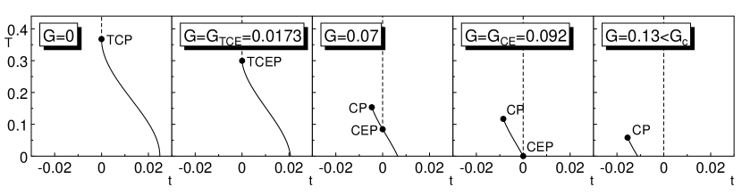
Figure 3: Phase diagrams of disordered itinerant ferromagnets in the $T$-$t$-plane showing first order (solid lines) and second order (dashed lines) transitions. $G$ is a dimensionless measure of the disorder, and CP, CEP, TCP, and TCEP denote critical points, critical endpoints, tricritical points and tricritical endpoints, respectively. The first panel corresponds to the experimental results on MnSi [46, 47]. See Ref. [64] for more details.

The properties of the continuous quantum phase transition occurring for stronger disorder can again be analyzed by standard renormalization group methods. It turns out that as in the clean case the Gaussian theory is sufficient since all higher order terms are irrelevant. The resulting critical exponents are $\gamma=1$ for all $d>2$ and $\nu=1/(d-2)$, $\eta=4-d$, $z=d$ for $2<d<4$. These exponents lock into their mean field values $\nu=1/2$, $\eta=0$, and $z=4$ for $d>4$. In addition to $d=4$, $d=6$ also plays the role of an upper critical dimension, and one has $\beta=2/(d-2)$, $\delta=d/2$ for $2<d<6$, while $\beta=1/2$, $\delta=3$ for $d>6$.

4 Influence of rare regions on magnetic quantum phase transitions

4.1 Disorder, rare regions, and the Griffiths region

The influence of static or quenched disorder on the critical properties of a system near a continuous phase transition is a very interesting problem in statistical mechanics. While it was initially suspected that quenched disorder always destroys any critical point [67], this was soon found to not necessarily be the case. Harris [68, 69] found a convenient criterion for the stability of a given critical behavior with respect to quenched disorder: If the correlation length exponent $\nu$ obeys the inequality $\nu\geq 2/d$, with $d$ the spatial dimensionality of the system, then the critical behavior is unaffected by the disorder. In the opposite case, $\nu<2/d$, the disorder modifies the critical behavior [70]. This modification may either (i) lead to a new critical point that has a correlation length exponent $\nu\geq 2/d$ and is thus stable, or (ii) lead to an unconventional critical point where the usual classification in terms of power-law critical exponents looses its meaning, or (iii) lead to the destruction of a sharp phase transition. The first possibility is realized in the conventional theory of random-$T_{c}$ classical ferromagnets [67], and the second one is probably realized in classical ferromagnets in a random field [71, 72, 73]. The third one has occasionally been attributed to the exactly solved McCoy-Wu model [74, 75, 76]. This is misleading, however, as has recently been emphasized in Ref. [77]; there is a sharp, albeit unorthodox, transition in that model, and it thus belongs to category (ii).

Independent of the question of if and how the critical behavior is affected, disorder leads to very interesting phenomena as a phase transition is approached. Disorder in general decreases the critical temperature $T_{c}$ from its clean value $T_{c}^{0}$. In the temperature region $T_{c}<T<T_{c}^{0}$ the system does not display global order, but in an infinite system one will find arbitrarily large regions that are devoid of impurities, and hence show local order, with a small but non-zero probability that usually decreases exponentially with the size of the region. These static disorder fluctuations are known as ‘rare regions’, and the order parameter fluctuations induced by them as ‘local moments’ or ‘instantons’. Since they are weakly coupled, and flipping them requires to change the order parameter in a whole region, the local moments have very slow dynamics. Griffiths [78] was the first to show that they lead to a non-analytic free energy everywhere in the region $T_{c}<T<T_{c}^{0}$, which is known as the Griffiths phase, or, more appropriately, the Griffiths region. In generic classical systems this is a weak effect, since the singularity in the free energy is only an essential one. An important exception is the McCoy-Wu model [74], which is a $2D$ Ising model with bonds that are random along one direction, but identical along the second direction. The resulting infinite-range correlation of the disorder in one direction leads to very strong effects. As the temperature is lowered through the Griffiths region, the local moments cause the divergence of an increasing number of higher order susceptibilities, $\partial^{n}m/\partial B^{n}$ ($n\geq 2$), starting with large $n$. Even the average susceptibility proper, $\chi^{(2)}=\partial m/\partial B$, diverges at a temperature $T_{\chi}>T_{c}$, although the average order parameter does not become non-zero until the temperature reaches $T_{c}$. This is caused by rare fluctuations in the susceptibility distribution, which dominate the average susceptibility and make it very different from the typical or most probable one.

Surprisingly little is known about the influence of the Griffiths region and related phenomena on the critical behavior. Recent work [79] on a random-$T_{c}$ classical Ising model has suggested that it can be profound, even in this simple model where the conventional theory predicts standard power-law critical behavior, albeit with critical exponents that are different from the clean case. The authors of Ref. [79] have shown that the conventional theory is unstable with respect to perturbations that break the replica symmetry. By approximately taking into account the rare regions, which are neglected in the conventional theory, they found a new term in the action that actually induces such perturbations. In some systems replica symmetry breaking is believed to be associated with activated, i.e. non-power law, critical behavior. Reference [79] thus raised the interesting possibility that, as a result of rare-region effects, the random-$T_{c}$ classical Ising model shows activated critical behavior, as is believed to be the case for the random-field classical Ising model [71, 72, 73], although in the case of the random-$T_{c}$ model no final conclusion about the fate of the transition could be reached.

Griffiths regions also occur in the case of quantum phase transitions (for an experimental example see Ref. [80]). Their consequences for the critical behavior are even less well investigated than in the classical case, with the remarkable exception of certain $1D$ systems. Fisher [77] has investigated quantum Ising spin chains in a transverse random field. These systems are closely related to the classical McCoy-Wu model, with time in the quantum case playing the role of the ‘ordered direction’ in the latter. He has found activated critical behavior due to rare regions. This has been confirmed by numerical simulations [81]. Other recent simulations [82] suggest that this type of behavior may not be restricted to $1D$ systems, raising the possibility that exotic critical behavior dominated by rare regions may be generic in quenched disordered quantum systems, independent of the dimensionality and possibly also of the type of disorder.

4.2 Itinerant quantum antiferromagnets

Within the conventional theory [67] of critical behavior in systems with quenched disorder the first step consists of averaging over the disorder, usually via the replica trick [83]. The resulting effective theory is then analyzed perturbatively. However, the rare regions are a non-perturbative effect since the probability for their occurrence is exponentially small in the disorder strength. Therefore, rare regions are neglected within the conventional theory.

Narayanan, Vojta, Belitz, and Kirkpatrick [84] have developed a generalization of the conventional theory of quantum phase transitions in the presence of quenched disorder. This theory, which is similar to that of Ref. [79] for classical transitions, includes the effects of the rare regions. The basic idea is not to average over the disorder at the beginning but to work with a particular disorder configuration until the rare regions are identified. Only after their effects have been incorporated into the theory, the disorder average is carried out.

In the following we illustrate this theory taking the itinerant quantum antiferromagnet as the primary example. The starting point is the order parameter field theory for the itinerant quantum antiferromagnet derived by Hertz [14]. The Landau-Ginzburg-Wilson free energy functional reads

$$S=\int dx\,dy\ {\mbox{\boldmath$\phi$}}(x)\,\Gamma_{0}(x,y)\,{\mbox{\boldmath$\phi$}}(y)+u\int dx\ \left({\mbox{\boldmath$\phi$}}(x)\cdot{\mbox{\boldmath$\phi$}}(x)\right)^{2}\,,$$ (37)

where $\phi$ is the staggered magnetization. $\Gamma(x,y)$ is the bare two-point vertex function, whose Fourier transform is

$$\Gamma_{0}({\bf q},\Omega_{n})=(t_{0}+{\bf q}^{2}+|\omega_{n}|)\quad.$$ (38)

Disorder is introduced by making the distance $t$ from the critical point a random function of position, $t({\bf x})=t_{0}+\delta t({\bf x})$, where $\delta t({\bf x})$ obeys a Gaussian distribution with zero mean and variance $\Delta$.

Instead of averaging over the disorder we now determine saddle point solutions of the unaveraged Landau-Ginzburg-Wilson functional (37). Due to the disorder there will be spatial regions in which the system wants to order ($t({\bf x})<0$) even if it is globally in its disordered phase ($t_{0}>0$). These rare regions or islands will support locally nonzero saddle-point solutions. Outside of the islands, the solution is exponentially small. Thus, the islands are effectively decoupled. For a system with $N$ islands, and in the case of Ising symmetry, there will be $2^{N}$ almost degenerate saddle-point solutions that can be constructed by considering all possible distributions of the sign of the order parameter on the islands. For a continuous order parameter symmetry there is a whole manifold of almost degenerate saddle points. This complicated structure of the free energy landscape is responsible for the failure of the conventional theory as is known from the random field Ising model [71, 72, 73].

Now, the crucial point is that for a complete theory one has to take into account fluctuations around all of these saddle points. As was shown in Ref. [84] the saddle point configurations act as an additional source of disorder in the system. Since the saddle points are time-independent this disorder is static, but it is self-generated and thus in equilibrium with the rest of the system. Therefore, taking into account fluctuations around all saddle points leads to the appearance of static annealed disorder in addition to the underlying quenched disorder. (Some general aspects concerning annealed disorder and quantum phase transitions are discussed in Ref. [85].) At this point in the calculation the average of the quenched disorder is carried out by means of the replica trick. The resulting effective theory for the fluctuations $\varphi$ takes the form

$${S}_{\rm eff} = ~{}\sum_{\alpha}\int dx\,dy\ \mbox{\boldmath$\varphi$}^{\alpha}(x)\,\Gamma_{0}(x,y)\,\mbox{\boldmath$\varphi$}^{\alpha}(y)+u\sum_{\alpha}\int dx\ \left(\mbox{\boldmath$\varphi$}^{\alpha}(x)\cdot\mbox{\boldmath$\varphi$}^{\alpha}(x)\right)^{2}$$ (39)

$$- \Delta\sum_{\alpha,\beta}\int dx\,dy\,\delta({\bf x}-{\bf y})\,\left(\mbox{\boldmath$\varphi$}^{\alpha}(x)\right)^{2}\,\left(\mbox{\boldmath$\varphi$}^{\beta}(y)\right)^{2}$$

$$- T{\bar{w}}\sum_{\alpha}\int dx\,dy\,\delta({\bf x}-{\bf y})\,\left(\mbox{\boldmath$\varphi$}^{\alpha}(x)\right)^{2}\,\left(\mbox{\boldmath$\varphi$}^{\alpha}(y)\right)^{2}~{}.$$

Here the first line represents the clean antiferromagnet, the second is the conventional quenched disorder term and the last line contains the static annealed disorder which is due to the rare regions. The temperature factor in front of the annealed disorder term originates from the Boltzmann factor for the saddle point free energy. The parameter $\bar{w}$ contains the probability for finding rare regions and the strength of the local order on the islands. Since $\bar{w}$ is non-perturbative in the disorder strength, the theory contains effects beyond the conventional perturbative approach.

This effective translationally invariant theory can now be analyzed by standard renormalization group methods. It turns out [84] that the new term in the Landau-Ginzburg-Wilson functional (39) destabilizes the critical fixed point found within the conventional theory [86]. No new fixed point is found (at one loop order of the perturbation theory). Instead, the system displays runaway flow to large disorder values in the entire physical parameter space. Within the renormalization group approach it is not possible to determine the ultimate fate of the transition. The runaway flow can be interpreted either as a complete destruction of the antiferromagnetic long-range order in favor of a random singlet phase [87, 88] or the existence of a non-conventional critical point (e.g., with activated scaling).

While rare regions destroy the conventional critical point in itinerant quantum antiferromagnets they do not influence the quantum phase transition of itinerant ferromagnets [84]. The reason is the effective long-ranged interaction between the order parameter fluctuations discussed in Sec. 3. It suppresses all fluctuations including those generated by the rare regions. Therefore the conventional critical behavior discussed in Subsec. 3.4 will not be changed by the rare regions.

5 Metal-insulator transitions of disordered interacting electrons

5.1 Localization and interactions

Metal-insulator transitions are a particularly fascinating and only incompletely understood class of quantum phase transitions. Conceptually, one distinguishes between Anderson transitions in models of noninteracting electrons, and Mott-Hubbard transitions of clean, interacting electrons. At the former, the electronic charge diffusivity $D$ is driven to zero by quenched, or frozen-in, disorder, while the thermodynamic properties do not show critical behavior. At the latter, the thermodynamic density susceptibility $\partial n/\partial\mu$ vanishes due to electron-electron interaction effects. In either case, the conductivity $\sigma=(\partial n/\partial\mu)D$ vanishes at the metal-insulator transition.

The investigation of the disorder-driven metal-insulator transition has a long history. Anderson [89] was the first to realize that introducing quenched disorder into a metallic system, e.g., by adding impurity atoms, can change the nature of the electronic states from spatially extended to localized. This localization transition of disordered non-interacting electrons, the Anderson transition, is comparatively well understood (for a review see, e.g., Ref. [90]). The scaling theory of localization [91] predicts that in the absence of spin-orbit coupling or magnetic fields all states are localized in one and two spatial dimensions for arbitrarily weak disorder. Thus, no true metallic phase exists in these dimensions. In contrast, in three dimensions there is a phase transition from extended states for weak disorder to localized states for strong disorder. These results of the scaling theory are in agreement with large-scale computer simulations of non-interacting disordered electrons.

However, in reality electrons do interact via the Coulomb potential, and the question is, how this changes the above conclusions. The conventional approach to the problem of disordered interacting electrons is based on a perturbative treatment of both disorder and interactions (for reviews see, e.g., Refs. [92, 93]). It leads to a scaling theory and a related field-theoretic formulation of the problem [94], which was later investigated in great detail within the framework of the renormalization group (for a review see Ref. [17]). One of the main results is that in the absence of external symmetry-breaking (spin-orbit coupling or magnetic impurities, or a magnetic field) a phase transition between a normal metal and an insulator only exists in dimensions larger than two, as was the case for non-interacting electrons. In two dimensions the results of this approach are inconclusive since the renormalization group displays runaway flow to zero disorder but infinite interactions. Furthermore, it has not been investigated so far, whether effects of rare regions analogous to those discussed in Sec. 4 for magnetic transitions would change the above conclusions about the metal-insulator transition.

Experimental work on the disorder-driven metal-insulator transition (mostly on doped semiconductors) carried out before 1994 essentially confirmed the existence of a transition in three dimensions while no transition was found in two-dimensional systems. Therefore it came as a surprise when experiments on Si-MOSFETs [95, 96] revealed indications of a true metal-insulator transition in two dimensions (see Fig. 4).

Figure 4: Resistivity of the 2D electron gas a Si-MOSFET as function of carrier concentration and doping. The data clearly indicate the existence of a metal-insulator transition. (from Ref. [96])

While these results were first viewed with considerable skepticism they were soon confirmed [97] and later also found in various other materials [98]. It soon became clear that the main difference between the new experiments and those carried out earlier was that the electron (or hole) density is very low. Therefore, the Coulomb interaction is particularly strong compared to the Fermi energy. For example, in the Si-MOSFETs the typical electron density is $10^{11}{\rm cm}^{-2}$ leading to a typical Coulomb energy of about 10 meV while the Fermi energy is only about 0.5 meV. Therefore interaction effects are a likely reason for this new metal-insulator transition in two dimensions. A complete understanding has, however, not yet been obtained. Different explanations have been suggested based on the perturbative renormalization group [100, 101], non-perturbative effects [102, 103], or the transition actually being a superconductor-insulator transition rather than a metal-insulator transition [104]. In addition to these interaction based explanations a number of more conventional suggestions have been made, among them the presence of temperature-dependent disorder as provided by the filling and emptying of charge traps [105] and temperature-dependent screening [106].

This is not the place to discuss all these developments in detail or even to review the vast field of metal-insulator transitions. Instead, we will concentrate on a few aspects of the metal-insulator transition in the presence of both disorder and interactions.

5.2 Rare regions, local moments, and annealed disorder, a new mechanism for the metal-insulator transition

In this subsection we discuss how rare regions analogous to those studied in Sec. 4 influence the metal-insulator transition. Let us consider an electron system in the presence of both interactions and (nonmagnetic) quenched disorder. Due to the disorder there will be rare spatial regions where the exchange interaction is greatly enhanced. In these regions the system will display local magnetic order. Physically, these regions correspond to local magnetic moments. There is much experimental evidence for local moments [107], and their formation has been studied theoretically [108].

Belitz, Kirkpatrick and Vojta [109] have developed an approach which includes the effects of the local moments into a transport theory, starting from a field-theoretical description of disordered interacting electrons. As in Sec. 4 the general idea is to avoid the disorder average at the beginning of the calculation but to work with a fixed disorder configuration. This leads to the appearance of spatially inhomogeneous saddle points of the field theory. In particular, there will be saddle points which have non-zero magnetization in some rare spatial regions. Analogous to Sec. 4 summing over the manifold of degenerate saddle points leads to the appearance of annealed magnetic disorder in addition to the underlying (nonmagnetic) quenched disorder. Let us emphasize that this annealed magnetic disorder is generically self-generated by the system.

In Ref. [109] the annealed magnetic disorder was then incorporated into the sigma-model description of the metal-insulator transition. To simplify the problem, a model of non-interacting electrons with annealed magnetic disorder was considered. This corresponds to neglecting all interaction effects beyond the formation of local moments. The resulting non-linear sigma model can be analyzed using the standard renormalization group methods [17]. It turns out that the annealed magnetic disorder leads to a new mechanism and a new universality class for the metal-insulator transition which is different from the conventional localization transition. Note that the effects of annealed magnetic disorder are also very different from the case of quenched magnetic impurities. For the simplified model and neglecting the Cooper channel we find that the diffusion coefficient is not renormalized at one loop order while the thermodynamic density susceptibility $\partial n/\partial\mu$ is driven to zero. Thus, the transition resembles a Mott-Hubbard transition rather than an Anderson transition.

The lower critical dimension for this new transition is two, as it is for the conventional localization transition. In two dimensions the system is insulating for any disorder. Therefore, the local moments alone do not provide an explanation for the metal-insulator transition in the two-dimensional electron system in Si-MOSFETs and other materials discussed in the last subsection. Clearly, it would be interesting to study generalizations of the model studied in Ref. [109] which include the Cooper channel and interactions beyond the formation of local moments.

5.3 Numerical simulation of disordered interacting electrons

The remaining part of Section 5 is devoted to the numerical work on interacting electrons in the presence of quenched disorder. The model investigated is the quantum Coulomb glass model [110, 111, 112], a generalization of the classical Coulomb glass model [113, 114] which was used to study disordered insulators. The quantum Coulomb glass is defined on a hypercubic lattice of $L^{d}$ sites occupied by $N=K\,L^{d}$ spinless electrons ($0\!<\!K\!<\!1$). To ensure charge neutrality each lattice site carries a compensating positive charge of $Ke$. The Hamiltonian is given by

$$H=-t\sum_{\langle ij\rangle}(c_{i}^{\dagger}c_{j}+c_{j}^{\dagger}c_{i})+\sum_{i}\varphi_{i}n_{i}+\frac{1}{2}\sum_{i\not=j}(n_{i}-K)(n_{j}-K)U_{ij}$$ (40)

where $c_{i}^{\dagger}$ and $c_{i}$ are the electron creation and annihilation operators at site $i$, respectively, and $\langle ij\rangle$ denotes all pairs of nearest neighbor sites. $t$ gives the strength of the hopping term and $n_{i}$ is the occupation number of site $i$. For a correct description of the insulating phase the Coulomb interaction between the electrons is kept long-ranged, $U_{ij}=U/r_{ij}$, since screening breaks down in the insulator (the distance $r_{ij}$ is measured in units of the lattice constant). The random potential values $\varphi_{i}$ are chosen independently from a box distribution of width $2W$ and zero average. Two important limiting cases of the quantum Coulomb glass are the Anderson model of localization (for $U_{ij}=0$) and the classical Coulomb glass (for $t=0$).

For two reasons the numerical simulation of disordered quantum many-particle systems is one of the most complicated problems in computational condensed matter physics. First, the dimension of the Hilbert space to be considered grows exponentially with the system size. Second, the presence of quenched disorder requires the simulation of many samples with different disorder configurations in order to obtain averages or distribution functions of physical quantities. In the case of disordered interacting electrons the problem is even more challenging due to the long-range character of the Coulomb interaction which has to be retained, at least for a correct description of the insulating phase. Here we discuss the results of two different numerical methods to tackle the problem. First, the Coulomb interaction is decoupled by means of a Hartree-Fock approximation and numerically solved the remaining self-consistent disordered single-particle problem. This method permits comparatively large system sizes of more than $10^{3}$ sites. The results of this approach are summarized in Sec. 5.4 together with those of exact diagonalization studies we performed to check the quality of the Hartree-Fock approximation. Since the Hartree-Fock method turned out to be a rather poor approximation for the calculation of transport properties an efficient method to calculate the low-energy properties of disordered quantum many-particle systems with high accuracy has been developed. This method, the Hartree-Fock based diagonalization, and the results we have obtained this way are summarized in Sec. 5.5.

5.4 Hartree-Fock approximation

The Hartree-Fock approximation consists in decoupling the Coulomb interaction by replacing operators by their expectation values:

$$H_{\rm HF}= - t\sum_{\langle ij\rangle}(c_{i}^{\dagger}c_{j}+c_{j}^{\dagger}c_{i})+\sum_{i}(\varphi_{i}-\mu)n_{i}$$ (41)

$$+ \sum_{i\not=j}n_{i}~{}U_{ij}\langle n_{j}-K\rangle-\sum_{i,j}c_{i}^{\dagger}c_{j}~{}U_{ij}\langle c_{j}^{\dagger}c_{i}\rangle,$$

where the first two terms contain the single-particle part of the Hamiltonian, the third is the Hartree energy and the fourth term contains the exchange interaction. $\langle\ldots\rangle$ represents the expectation value with respect to the Hartree-Fock ground state which has to be determined self-consistently. In this way the many-particle problem is reduced to a self-consistent disordered single-particle problem which we solve by means of numerically exact diagonalization.

This method was applied to the three-dimensional quantum Coulomb glass model [112]. It was found that the interaction induces a depletion of the single-particle density of states in the vicinity of the Fermi energy. For small hopping strength $t$ the depletion takes the form of a Coulomb gap [114, 115] known from the classical ($t=0$) limit. With increasing hopping strength there is a crossover from the nearly parabolic Coulomb gap to a square root singularity characteristic of the Coulomb anomaly [116] in the metallic limit. The depletion of the density of states at the Fermi energy has drastic consequences for the localization properties of the electronic states. Since the degree of localization is essentially determined by the ratio between the hopping amplitude and the level spacing, a reduced density of states directly leads to stronger localization. Specifically, we calculated the inverse participation number

$$P_{\nu}^{-1}=\sum_{j}|\langle j|\nu\rangle|^{4}$$ (42)

of a single-particle state $|\nu\rangle$ and compared the cases of non-interacting and interacting electrons. In the presence of interactions we found a pronounced maximum at the Fermi energy with values above that of non-interacting electrons. Thus, within the Hartree-Fock approximation electron-electron interactions lead to enhanced localization.

In order to precisely determine how the location of the metal-insulator transition changes as a result of this effect, we used the fact that the spectral statistics on the insulating side is equivalent to that of a Poisson ensemble of random matrices while the spectral statistics on the metallic side is that of a Gaussian orthogonal ensemble of random matrices [117, 118]. By analyzing the statistics of the Hartree-Fock levels as a function of the hopping amplitude $t$ we could thus determine the location of the metal-insulator transition in the phase diagram. In all cases the transition to a metal requires a larger hopping strength for interacting electrons than for non-interacting.

Since the Hartree-Fock method is an uncontrolled approximation it is highly desirable to compare these results to those of exact many-particle calculations. Now the question arises, what quantities are particular suitable for such a comparison. In principle, one should compare the values of physical observables like the conductivity which is given by the Kubo-Greenwood formula [121, 122]

$${\rm Re}~{}G^{xx}(\omega)=\frac{2\pi^{2}}{\omega}\sum_{\nu}|\langle 0|j^{x}|\nu\rangle|^{2}\delta(\omega+E_{0}-E_{\nu})$$ (43)

where $\omega$ denotes the frequency. $j^{x}$ is the $x$ component of the current operator and $|\nu\rangle$ denotes the eigenstates of the Hamiltonian. However, the Kubo-Greenwood conductivity is a complicated quantity from a numerical point of view since it involves a nontrivial extrapolation to zero frequency. Therefore, it is desirable to apply the simpler localization criteria known from non-interacting systems. This leads, however, to an additional complication. The usual criteria which are based on the (single-particle) participation number or the statistics of (single-particle) energy levels are not even defined for many-particle states. While this does not create any problems at the Hartree-Fock level (the Hartree-Fock states are effective single-particle states) it implies that the criteria cannot directly be applied to true many-particle states. There have been several suggestions (for a discussion see Ref. [119]) how to generalize the participation number to a many-particle state. It turns out that a unique procedure does not exist, and different generalizations have different merits. Since localization is connected with the probability of a particle to return to its starting position, a promising candidate to replace the inverse participation number is

$$R_{p}(\varepsilon)=\frac{1}{g(\varepsilon)}\frac{1}{N}\sum_{j}\lim_{\delta\to 0}\frac{\delta}{\pi}\,G_{jj}(\varepsilon+i\delta)\,G_{jj}(\varepsilon-i\delta)~{}.$$ (44)

Here $g(\varepsilon)$ is the single-particle density of states and $G_{jj}$ is the diagonal element of the single-particle Greens function. This quantity measures the probability of a single particle excitation created at site $j$ to return to this site in infinite time. However, in addition to the desired localization information $R_{p}$ also contains information about the decay of the quasi-particles. To disentangle localization and decay information we note that the quasi-particle weight $z_{0}$ (which measures the decay only) can be expressed as

$$z_{0}^{2}(\varepsilon)=\frac{1}{g(\varepsilon)}\frac{1}{N}\sum_{ij}\lim_{\delta\to 0}\frac{\delta}{\pi}\,G_{ij}(\varepsilon+i\delta)\,G_{ji}(\varepsilon-i\delta)~{}.$$ (45)

The desired localization information is thus contained in the normalized return probability $P^{-1}=R_{p}/z_{0}^{2}$ which is the natural generalization of the inverse participation number (42) to interacting systems. For non-interacting electrons it reduces to the inverse participation number proper.

Using these criteria the Hartree-Fock results were compared [120] to those of numerically exact diagonalizations of the many-particle Hamiltonian. Because the exact calculations require the diagonalization of a matrix whose dimension equals the size of the Hilbert space this comparison was restricted to systems with not more than 16 sites. While it was found that the Hartree-Fock approximation yields reasonable results for static quantities like the single-particle density of states, it does a very poor job for localization properties and for time correlation functions such as the conductivity. Thus, the Hartree-Fock results for the influence of the electron-electron interaction on transport quantities are highly unreliable. For this reason it was necessary to develop a new numerical method, the Hartree-Fock based diagonalization which will be discussed in the next subsection.

5.5 Hartree-Fock based diagonalization

Since numerically exact diagonalizations of the full many-particle Hamiltonian are restricted to very small system sizes and, as we have seen, the Hartree-Fock results for transport properties are unreliable, a different method which gives exact results or at least provides a controlled approximation for comparatively large systems is highly desirable. Such a method is the Hartree-Fock based diagonalization [123]. It is related to the configuration interaction (CI) approach used in quantum chemistry (see, e.g., Ref. [124]). The basic idea is to diagonalize the many-particle Hamiltonian not in a real-space or momentum basis but rather in an energetically truncated basis of Hartree-Fock states. The Hartree-Fock states are comparatively close in character to the exact eigenstates in the entire parameter space. Therefore it is sufficient to keep only a very small fraction of the Hilbert space (e.g., 2000 out of $9\times 10^{9}$ states for 18 electrons on 36 lattice sites) to obtain low-energy quantities with an accuracy comparable to that of exact diagonalization. A schematic of the Hartree-Fock based diagonalization method is shown in Fig. 5.

do for each disorder configuration solve HF approximation construct many-particle HF states find lowest-in-energy HF states transform Hamiltonian to basis of low-energy HF states diagonalize Hamiltonian transform observables to HF basis and calculate their values enddo

Figure 5: Structure of the Hartree-Fock (HF) based diagonalization method.

So far we have carried out test calculations for systems with up to 64 lattice sites (32 electrons) and production runs for up to 36 lattice sites (18 electrons).

As a first application of the Hartree-Fock based diagonalization method the quantum Coulomb glass was studied in two dimensions [125]. In order to determine the influence of the Coulomb interaction on transport the Kubo-Greenwood conductance (43) was calculated. It turned out that the influence of electron-electron interactions on the d.c. conductance is opposite in the weakly and strongly disordered regimes. The conductance of strongly disordered electrons is considerably enhanced by a weak interactions. With increasing kinetic energy the relative enhancement decreases as does the interaction range where the enhancement occurs. The conductance of weakly disordered electrons is reduced even by weak interactions. In contrast, sufficiently strong interactions always reduce the conductance, and the system approaches a Wigner crystal or Wigner glass state. These results are summarized in Fig. 6.

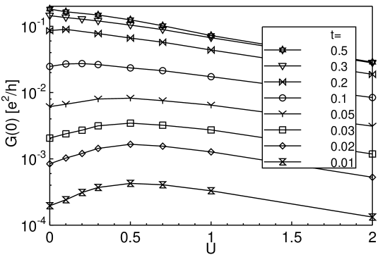
Figure 6: d.c. conductance of a 2D system of $5\times 5$ sites. The disorder strength is $W=1$. The results represent logarithmic averages over 400 disorder configurations. (from Ref. [125])

The qualitative difference we found between the weakly and strongly disordered regimes can be explained in terms of two competing effects of the interactions. The dominant effect in the case of strong disorder is the destruction of phase coherence for the single-electron motion. It can be understood from the following simplistic argument: Electron-electron collisions are inelastic and thus phase-breaking from the point of view of a single electron. Therefore collisions destroy the quantum interference necessary for Anderson localization. It is clear that this mechanism to increase the conductance is particularly effective if the localization length is very small to begin with. In the opposite case, i.e., for weak disorder, the dominant effect of the interactions is an increasing pinning of the electrons by the repulsive forces which for strong interactions eventually leads to the formation of a Wigner glass or crystal. This simple arguments also explain, why the Hartree-Fock approximation did not reproduce the enhanced conductance in the localized regime: The Hartree-Fock potential is static and therefore it does not break the phase of the electron – in contrast to real electron-electron collisions.

Analogous investigations were performed for quantum Coulomb glasses in three [126] and one [127] spatial dimensions. It turned out that the qualitative disorder and interaction dependencies of the conductance are identical to those in two dimensions. In particular, it was always found that weak interactions induce delocalization in the strongly disordered regime. The degree of delocalization seems to be determined essentially by the ratio between disorder strength $W$ and the hopping band width $zt$ where $z$ is the number of nearest neighbor sites. In addition to the results obtained by the HFD method, other numerical simulations also show a delocalizing influence of electron-electron interactions in one [128] and two [110, 111, 129, 130] dimensions. The numerical results for the influence of weak interactions on the Kubo-Greenwood conductance can be compared to the results from the perturbative renormalization group for spinless fermions [131] which predicts that repulsive interactions always reduce the transport of disordered spinless fermions. Thus, the numerical results agree with those from perturbation theory in the case of weak disorder, while in the strongly disordered regime the perturbative results are qualitatively incorrect.

In addition to the Kubo-Greenwood conductance the above mentioned return probability of single-particle excitations was also calculated. The return probability at the Fermi energy displays a similar behavior as the Kubo-Greenwood conductance: For weak disorder the return probability increases with the interaction strength. The delocalizing tendency in the strongly localized regime is less pronounced, probably because the Coulomb gap in the single-particle density of states counteracts the delocalization.

In summary, the results obtained so far clearly show that interactions can have a delocalizing tendency in certain parameter regions. However, it is not clear whether this is sufficient to explain the metal-insulator transition found in two dimensions. More detailed investigations are presently under way to find the finite-size scaling behavior of the conductance. Moreover, we are currently generalizing the simulations to include spin degrees of freedom which have been shown to be important in the experiments on Si-MOSFETs [132, 133].

6 Summary and outlook

In this review we have discussed quantum (or zero temperature) phase transitions in electronic systems. After a pedagogical introduction on the similarities and differences between classical thermal and quantum phase transitions we have considered three specific examples in some detail: quantum phase transitions in the spherical model, magnetic quantum phase transitions of itinerant electrons, and some aspects of the disorder-driven metal-insulator transition. In this final chapter we want to summarize the results from a common perspective and discuss some of the remaining open questions as well as future research directions.

The theoretical description of a particular phase transition occurring in nature usually starts with the identification of the relevant variables, the most important one being the order parameter. To proceed further, analytical investigations often follow the Landau-Ginzburg-Wilson philosophy, i.e., all degrees of freedom other than the order parameter fluctuations are integrated out, resulting in an effective theory in terms of the order parameter only. If a rigorous analytical derivation is complicated, the Landau-Ginzburg-Wilson theory is sometimes guessed based on general symmetry considerations. (This is true in particular when constructing toy models like the quantum spherical model.) However, our work on the ferromagnetic quantum phase transition has shown that great care has to be taken in such an approach. At zero temperature an electronic system usually contains many non-critical soft modes in addition to the critical order parameter fluctuations. If these soft modes couple to the order parameter integrating them out leads to a singular behavior in the Landau-Ginzburg-Wilson theory. This mechanism is not restricted to zero temperature. Any soft mode coupling to the order parameter can – when integrated out – produce singularities in the resulting Landau-Ginzburg-Wilson theory. However, in electronic systems the number of soft modes at zero temperature is much higher than at finite temperatures.

In the case of itinerant ferromagnets we have shown that these singularities result either in unusual non-mean-field scaling behavior at the quantum phase transition or in the quantum phase transition being of first order (as is the case experimentally for the transition in MnSi). Within the singular Landau-Ginzburg-Wilson theory it is very hard to find out what scenario is realized for what microscopic parameters since explicit calculations are next to impossible. A much more promising though technically more challenging approach consists in not integrating out all degrees of freedom other than the order parameter. Instead, the effective field theory should treat all soft modes in the system on the same footing. We will explore the merits of such an approach in the future.

Another potential problem of the standard approach is caused by the fact that it is based on perturbation theory: First, integrating out the microscopic degrees of freedom in the derivation of the Landau-Ginzburg-Wilson theory can usually be done only perturbatively. Second, the analysis of the effective theory is done by means of the perturbative renormalization group. Now, if the free energy landscape in configuration space contains many, nearly degenerate minima separated by large barriers, as for instance in the presence of random interactions or random fields, a straight-forward perturbative approach may miss part of the physics. We have shown this explicitly for the antiferromagnetic quantum phase transition of weakly disordered itinerant electrons. By approximately taking into account the non-perturbative degrees of freedom connected with the many nearly degenerate free energy minima we have derived a correction to the effective action of the standard perturbative approach. This correction takes the form of static annealed disorder. Including the new term into the renormalization group destabilizes the conventional critical behavior. However, within our theory the ultimate fate of the transition could not be determined. Further work will be necessary to decide between the different possibilities, viz., a complete destruction of the antiferromagnetic long-range order or an unconventional transition that may be characterized by an infinite-disorder fixed point and activated scaling.

It should be emphasized here that we have also shown that including the non-perturbative degrees of freedom connected with the many-valley structure of the free energy in the presence of disorder does not always destroy the conventional critical behavior. For itinerant quantum ferromagnets, for instance, the long-range interaction between the order parameter fluctuations stabilizes the conventional critical fixed point. In principle, the method we used to include rare regions into magnetic quantum phase transitions of disordered itinerant electrons can be applied to any quantum phase transition in the presence of quenched disorder. In the case of the disorder-driven metal-insulator transition we found that magnetic rare regions (which physically correspond to local magnetic moments) can lead to a new mechanism and a new universality class for the transition. In the simplified model investigated so far (which neglects all interaction effects beyond local moments) no transition was found in two dimensions. An obvious question would be whether this conclusions changes for a more realistic model.

An alternative way to go beyond perturbation theory are numerical simulations. We have chosen this approach for an investigation of the metal-insulator transition in the presence of both interactions and quenched disorder. We have developed an efficient numerical method, the Hartree-Fock based diagonalization method which is related to the configuration interaction approach used in quantum chemistry. It allows us to calculate with high accuracy the low-energy properties of disordered interacting electrons for moderately large systems. So far, we have mostly obtained qualitative results concerning the influence of the electron-electron interactions on the transport properties: For systems of spinless fermions the interactions reduce the d.c. conductance for weak disorder (in agreement with perturbative results) while they enhance the d.c. conductance for strong disorder. In future work we plan to extend this work to a systematic finite-size scaling study which will lead to quantitative results about the metal-insulator transition. Moreover, we are working on including the spin degrees of freedom into our numerical scheme. This is of particular importance since the spin degrees of freedom have proven to be crucial for the recently discovered metal-insulator transition in two dimensions.

The work presented here would have been impossible without the contributions of many friends and colleagues. I particularly thank my collaborators on the magnetic transitions, D. Belitz, T. R. Kirkpatrick, R. Narajanan and A. Millis. Equal thanks go to M. Schreiber and F. Epperlein for the collaboration on the numerical part of the work. I greatly appreciated discussions with Alexei Efros, Ferdinand Evers, Roger Haydock, Svetlana Kilina, Bernhard Kramer, Arnulf Möbius, Christian Pfleiderer, Michael Pollak, Rudolf Römer, Achim Rosch, Walter Schirmacher, Jorge Talamantes, John Toner, Matthias Vojta, Dietmar Weinmann, and Isa Zarekeshev.

This work was supported in part by the DFG (Vo659/1, SFB 393/C2) and by the NSF (DMR-95-10185, DMR-98-70597). The author is also grateful to the Aspen Center for Physics, where part of the work has been performed.

References

- [1] T. Andrews, Phil. Trans. R. Soc. 159 (1869) 575
- [2] J. D. van der Waals, PhD thesis, University of Leiden 1873
- [3] P. Curie, Ann. Chim. Phys. 5 (1895) 289
- [4] P. Weiss, J. Phys. Radium (Paris) 6 (1907) 667
- [5] L. D. Landau, Phys. Z. Sowjun. 11 (1937) 26; ibid 545; Zh. Eksp. Teor. Fiz 7 (1937) 19; ibid 627
- [6] E. A. Guggenheim, J. Chem. Phys. 13 (1945) 253
- [7] L. Onsager, Phys. Rev. 65 (1944) 117
- [8] B. Widom, J. Chem. Phys. 43 (1965) 3892
- [9] L. P. Kadanoff, Physics 2 (1966) 263
- [10] K. G. Wilson, Phys. Rev. B 4 (1971) 3174; ibid 3184
- [11] P. Meakin, Phys. Rep. 235 (1993) 189
- [12] J. Marro and R. Dickman, Non-equilibrium phase transitions in lattice models, Cambridge University Press, Cambridge 1997
- [13] H. van Beijeren (Editor), Proc. 9th Int. Summerschool on Fundamental Problems in Statistical Mechanics, Phys. Rep. 301 (1998) nos. 1–3
- [14] J. A. Hertz, Phys. Rev. B 14 (1976) 1165
- [15] M. Suzuki, Progr. Theor. Phys. 56 (1976) 1454
- [16] M. T. Beal-Monod, Solid State Commun. 14 (1974) 677
- [17] D. Belitz and T. R. Kirkpatrick, Rev. Mod. Phys. 66 (1994) 261
- [18] S. Sachdev, in Proc. 19th IUPAP Int. Conf. on Statistical Physics edited by H. Bailin, World Scientific, Singapore 1996, p.289
- [19] S. L. Sondhi, S. M. Girvin, J. P. Carini, and D. Shahar, Rev. Mod. Phys. 69 (1997) 315
- [20] T. R. Kirkpatrick and D. Belitz, in Electronic correlations in the solid state edited by N. H. March, to be published by Imperial College Press, cond-mat/9707001
- [21] D. Belitz and T. R. Kirkpatrick, in Models and kinetic methods for non-equilibrium many-body systems edited by J. Karkheck, Kluwer Academic, Dordrecht 1998
- [22] S. Sachdev and M. Vojta, cond-mat/9908008
- [23] S. Sachdev, Quantum phase transitions, Cambridge University Press, Cambridge 1999
- [24] S.-K. Ma, Modern Theory of Critical Phenomena, Benjamin, Reading 1976
- [25] N. Goldenfeld, Lectures on phase transitions and the renormalization group, Addison-Wesley, Reading 1992
- [26] V. L. Ginzburg, Sov. Phys. – Sol. State 2 (1960) 1824
- [27] S. Chakravarty, B. I. Halperin, and D. R. Nelson, Phys. Rev. B 39 (1989) 2344
- [28] T. H. Berlin and M. Kac, Phys. Rev. 86 (1952) 821
- [29] H. E. Stanley, Phys. Rev. 176 (1968) 718
- [30] G. S. Joyce, Phys. Rev. 146 (1966) 349
- [31] J. M. Kosterlitz, D. J. Thouless, and R. C. Jones, Phys. Rev. Lett. 36 (1976) 1217
- [32] A. Jagannathan and J. Rudnick, J. Phys. A 22 (1989) 513
- [33] R. M. Hornreich and H. G. Schuster, Phys. Rev. B 26 (1982) 3929
- [34] T. Vojta, J. Phys. A 26 (1993) 2883; T. Vojta and M. Schreiber, Phys. Rev. B 50 (1994) 1272
- [35] T. Vojta and M. Schreiber, Phys. Rev. B 49 (1994) 7861
- [36] M. E. Fisher and M. N. Barber, Phys. Rev. Lett. 28 (1972) 1516
- [37] J. Rudnick, in Finite Size Scaling and Numerical Simulation of Statistical Systems, edited by V. Privman, World Scientific, Singapore 1990, p.141
- [38] G. S. Joyce, in Phase Transitions and Critical Phenomena vol. 2 edited by C. Domb and M. S. Green, Academic Press, New York 1972
- [39] A. M. Khorunzhy, B. A. Khoruzhenko, L. A. Pastur, and M. V. Shcherbina, in Phase Transitions and Critical Phenomena vol. 15 edited by C. Domb and J. Lebowitz, Academic Press, New York 1992
- [40] G. Obermair, in Dynamical aspects of critical phenomena edited by J. I. Budnick and M. P. Kawatra, Gordon and Breach, New York 1972
- [41] T. M. Nieuwenhuizen, Phys. Rev. Lett. 74 (1995) 4293
- [42] T. Vojta, Phys. Rev. B 53 (1996) 710
- [43] T. Vojta and M. Schreiber, Phys. Rev. B 53 (1996) 8211
- [44] L. D. Landau, Zh. Eksp. Teor. Fiz 30 (1956) 1058 [Sov. Phys. JETP 3 (1956) 920]
- [45] L. D. Landau, Zh. Eksp. Teor. Fiz 32 (1957) 59 [Sov. Phys. JETP 5 (1957) 101]
- [46] C. Pfleiderer, G. J. McMullan, and G. G. Lonzarich, Physica B 206&207 (1995) 847
- [47] C. Pfleiderer, G. J. McMullan, S. R. Julian, and G.G. Lonzarich, Phys. Rev. B 55 (1997) 8330, and references therein
- [48] K. Adachi et al., J. Phys. Soc. Japan 47 (1979) 675
- [49] T. Sakakibara, T. Goto, K. Yoshimura, and K. Fukamichi J. Phys. Condens. Matter 2 (1990) 3381
- [50] A. J. Millis, Phys. Rev. B 48 (1993) 7183
- [51] T. Moriya, Spin fluctuations in itinerant electron magnetism, Springer, Berlin 1985
- [52] S. Sachdev, Z. Phys. B 94 (1994) 469
- [53] T. Vojta, D. Belitz, R. Narayanan, and T. R. Kirkpatrick, Europhys. Lett. 36 (1996), 191
- [54] T. Vojta, D. Belitz, R. Narayanan, and T. R. Kirkpatrick, Z. Phys. B 103 (1997) 451
- [55] J. W. Negele and H. Orland, Quantum many-particle systems, Addison-Wesley, New York 1988
- [56] J. Hubbard, Phys. Rev. Lett. 3 (1959) 77
- [57] R. L. Stratonovich, Dokl. Akad. Nauk SSSR 115 (1957) 1907 [Sov. Phys. Dokl. 2 (1957) 416]
- [58] E. C. Stoner, Proc. Roy. Soc. A 165 (1938) 372
- [59] D. Belitz, T. R. Kirkpatrick, and T. Vojta, Phys. Rev. B 55 (1997) 9452
- [60] B. Schmittmann and R. K. P. Zia, Phys. Rep. 301 (1998) 45
- [61] P. C. Hohenberg and B. I. Halperin, Rev. Mod. Phys. 49 (1977) 435
- [62] R. M. White, Quantum Theory of Magnetism, McGraw-Hill, New York 1970
- [63] T. Vojta, D. Belitz, T.R. Kirkpatrick, R. Narayanan, Ann. Phys. (Leipzig) 8 (1999) 593
- [64] D. Belitz, T. R. Kirkpatrick and T. Vojta, Phys. Rev. Lett 82 (1999) 4707
- [65] D. Belitz, T. R. Kirkpatrick, A. Millis, and T. Vojta, Phys. Rev. B 58 (1998) 14155
- [66] T. R. Kirkpatrick and D. Belitz, Phys. Rev. B 53 (1996) 14364
- [67] For a pedagogical discussion, see, G. Grinstein, in Fundamental Problems in Statictical Mechanics VI, edited by E. G. D. Cohen, Elsevier, New York 1985, p.147, and references therein
- [68] A. B. Harris, J. Phys. C 7 (1974) 1671 (1974)
- [69] J. Chayes, L. Chayes, D. S. Fisher, and T. Spencer, Phys. Rev. Lett. 57 (1986) 2999
- [70] For a recent discussion concerning the validity of the Harris criterion, see, F. Pazamandi, R. T. Scalettar, and G. Zimanyi, Phys. Rev. Lett. 79 (1997) 5130; S. Wiseman and E. Domany, Phys. Rev. Lett. 81 (1998) 22; A. Aharony, A. B. Harris, and S. Wiseman, Phys. Rev. Lett. 81 (1998) 252
- [71] J. Villain, J. Phys. (Paris) 46 (1985) 1843
- [72] D. S. Fisher, Phys. Rev. Lett. 56 (1986) 416
- [73] A. E. Nash, A. R. King, and V. Jaccarino, Phys. Rev. B 43 (1991) 1272
- [74] B. M. McCoy and T. T. Wu, Phys. Rev. 176 (1968) 631; ibid 188 (1969) 982
- [75] B. M. McCoy, Phys. Rev. 188 (1969) 1014
- [76] R. Shankar and G. Murthy, Phys. Rev. B 36 (1987) 536
- [77] D. S. Fisher, Phys. Rev. B 51 (1995) 6411
- [78] R. B. Griffiths, Phys. Rev. Lett. 23 (1969) 17
- [79] V. Dotsenko, A. B. Harris, D. Sherrington, and R. B. Stinchcombe, J. Phys. A 28 (1995) 3093
- [80] M. C. de Andrade, R. Chau, R. P. Dickey, N. R. Dilley, E. J. Freeman, D. A. Gajewski, M. B. Maple, R. Movshovich, A. H. Castro Neto, and G. Castilla, Phys. Rev. Lett. 81 (1998) 5620
- [81] J. Kisker and A.P. Young, Phys. Rev. B 58 (1998) 14397
- [82] C. Pich, A. P. Young, H. Rieger, and N. Kawashima, Phys. Rev. Lett. 81 (1998) 5916
- [83] S. F. Edwards and P. W. Anderson, J. Phys. F 5 (1975) 965
- [84] R. Narayanan, T. Vojta, D. Belitz, and T. R. Kirkpatrick, Phys. Rev. Lett. 82 (1999) 5132; Phys. Rev. B 60 (1999) 10150
- [85] R. Narayanan, T. Vojta, D. Belitz and T.R. Kirkpatrick, Ann. Phys. (Leipzig) 8 (1999) SI–185
- [86] T. R. Kirkpatrick and D. Belitz, Phys. Rev. Lett. 76 (1996) 2571; ibid 78 (1997) 1197
- [87] R. N. Bhatt and P. A. Lee, Phys. Rev. Lett. 48 (1982) 344
- [88] R. N. Bhatt and D. S. Fisher, Phys. Rev. Lett. 68 (1992) 3072
- [89] P. W. Anderson, Phys. Rev. 109 (1958) 1492
- [90] B. Kramer and A. MacKinnon, Rep. Progr. Phys. 56 (1993) 1469
- [91] E. Abrahams, P. W. Anderson, D. C. Licciardello, and T. V. Ramakrishnan, Phys. Rev. Lett. 42 (1979) 637
- [92] B. L. Altshuler and A. G. Aronov, in Electron-electron interactions in disordered systems edited by A. L. Efros and M. Pollak, North-Holland, Amsterdam 1985
- [93] P. A. Lee and T. V. Ramakrishnan, Rev. Mod. Phys. 57 (1985) 287
- [94] A. M. Finkelstein, Zh. Eksp. Teor. Fiz. 84 (1983) 168 [Sov. Phys. JETP 57 (1983) 97]
- [95] S. V. Kravchenko, G. V. Kravchenko, J. E. Furneaux, V. M. Pudalov, and M. D’Iorio, Phys. Rev. B 50 (1994) 8039
- [96] S. V. Kravchenko, W. E. Mason, G. E. Bowker, J. E. Furneaux, V. M. Pudalov, and M. D’Iorio, Phys. Rev. B 51 (1995) 7038
- [97] D. Popovich, A. B. Fowler, and S. Washburn, Phys. Rev. Lett. 79 (1997) 1543
- [98] P.T. Coleridge, R.L. Williams, Y. Feng, and P. Zawadski, Phys. Rev. B 56 (1997) R12764; Y. Hanein, U. Meirav, D. Shahar, C. C. Li, D. C. Tsui, and H. Shtrikman, Phys. Rev. Lett 80 (1998) 1288; M. Y. Simmons, A. R. Hammilton, M. Pepper, E. H. Linfield, P. D. Rose, D. A. Richie, A. K. Savchenko, and T. G. Griffiths, Phys. Rev. Lett. 80 (1998) 1292
- [99] M. Y. Simmons, A. R. Hamilton, M. Pepper, E. H. Linfield, P. D. Rose, and D. A. Ritchie, cond-mat/9910368
- [100] C. Castellani, C. DiCastro and P. A. Lee, Phys. Rev. B 57 (1998) R9381
- [101] Q. Si and C. M. Varma, Phys. Rev. Lett. 81 (1998) 4951
- [102] S. Chakravarty, L. Yin, and E. Abrahams, Phys. Rev. B 58 (1998) R559
- [103] S. Chakravarty, S. Kivelson, C. Nayak, and K. Völker, Phil. Mag. B 79 (1999) 859
- [104] D. Belitz and T. R. Kirkpatrick, Phys. Rev. B 58 (1998) 8214; P. Phillips, Y. Wan, I Martin, S. Knych, and D. Dalidovich, Nature 395 (1998) 253; F. C. Zhang and T. M. Rice, cond-mat/9708050
- [105] B. L. Altshuler and D. L. Maslov, Phys. Rev. Lett. 82 (1999) 145
- [106] T. M. Klapwijk and S. Das Sarma, Solid State Commun. 110 (1999) 581
- [107] M. A. Paalanen, S. Sachdev, R. N. Bhatt, and A. E. Ruckenstein, Phys. Rev. Lett. 57 (1986) 2061; M. A. Paalanen, J. E. Graebner, R. N. Bhatt, and S. Sachdev, Phys. Rev. Lett. 61 (1988) 597
- [108] M. Milovanovic, S. Sachdev, and R.N. Bhatt, Phys. Rev. Lett. 63 (1989) 82, and references therein
- [109] D. Belitz, T. R. Kirkpatrick, and T. Vojta, cond-mat/9910040
- [110] A. L. Efros and F. G. Pikus, Solid State Commun. 96 (1995) 183
- [111] J. Talamantes, M. Pollak, and L. Elam, Europhys. Lett. 35 (1996) 511
- [112] F. Epperlein, M. Schreiber, and T. Vojta, Phys. Rev. B 56 (1997) 5890
- [113] M. Pollak, Discuss. Faraday Soc. 50 (1970) 13
- [114] A. L. Efros and B. I. Shklovskii, J. Phys. C 8 (1975) L49
- [115] A. L. Efros and B. I. Shklovskii, in Electron-electron interactions in disordered systems, edited by A. L. Efros and M. Pollak, North-Holland, Amsterdam 1985, p.409
- [116] B. L. Altshuler and A. G. Aronov, Sol. State Commun. 30 1979 115
- [117] B. I. Shklovskii, B. Shapiro, B. R. Sears, P. Lambrianides, and H. B. Shore, Phys. Rev. B 47 (1993) 11487
- [118] E. Hofstetter and M. Schreiber, Phys. Rev. B 48 (1993) 16979
- [119] T. Vojta, F. Epperlein, and M. Schreiber, phys. stat. sol. (b) 205 (1998) 53
- [120] F. Epperlein, M. Schreiber, and T. Vojta, phys. stat. sol. (b) 205 (1998) 233
- [121] K. Kubo, J. Phys. Soc. Jpn. 12 (1957) 576
- [122] D. A. Greenwood, Proc. Phys. Soc., London 71 (1958) 585
- [123] T. Vojta, F. Epperlein, and M. Schreiber, to appear in Computer Phys. Commun., cond-mat/9809171
- [124] P. Fulde, Electron correlations in molecules and solids, Springer, Berlin 1995
- [125] T. Vojta, F. Epperlein, and M. Schreiber, Phys. Rev. Lett. 81 (1998) 4212
- [126] T. Vojta and F. Epperlein, Ann. Phys. (Leipzig) 7 (1998) 493
- [127] M. Schreiber, F. Epperlein, and T. Vojta, Physica A 266 (1999) 443
- [128] P. Schmitteckert, R. A. Jalabert, D. Weinmann, and J. L. Pichard, Phys. Rev. Lett. 81 (1998) 2308
- [129] G. Benenti, X. Waintal, and J. L. Pichard, Phys. Rev. Lett. 83 (1999) 1826
- [130] P. J. H. Denteneer, R. T. Scalettar, and N. Trivedi, cond-mat/9907246
- [131] W. Apel and T. M. Rice, Phys. Rev. B 26 (1982) 7063
- [132] D. Simonian, S. V. Kravchenko, and M. P. Sarachik, ibid. 79 (1997) 2304
- [133] V. M. Pudalov, G. Brunthaler, A. Prinz, and G. Bauer, JETP Lett. 65 (1997) 932