Kinetic equation for liquids with a multistep potential of interaction. II: Calculation of transport coefficients

Abstract

We consider a new kinetic equation for systems with a multistep potential of interaction proposed by us recently in Physica A 234 (1996) 89. This potential consists of the hard sphere part and a system of attractive and repulsive walls. Such a model is a generalization of many previous semi-phenomenological kinetic theories of dense gases and liquids. In this article a normal solution to the new kinetic equation has been obtained, integral conservation laws in the first order on gradients of hydrodynamic parameters have been derived as well. The expressions for transport coefficients are calculated for the case of stationary process. We also consider limiting cases for this kinetic equation. For specific parameters of model interaction potential in shape of the multistep function, the obtained results rearrange to those of previous kinetic theories by means of the standard Chapman-Enskog method. In view of this, new theory can be considered as a generalized one which in some specific cases arrives at the results of previous ones and in such a way displays the connection of these theories between themselves. At the end of this article we present results of numerical computation of transport coefficients for Argon along curve of saturation and their comparison with experimental data available and MD simulations.

1 Introduction

The main problem of kinetic theory in the last few decades was to appreciate properties of dense gases and liquids on the basis of motion laws and molecular interactions. In 1872 L.Boltzmann suggested a kinetic equation for a dilute gas [1]. At the same time, he constructed the entropy functional and proved $H$-theorem.

In 1946, N.N.Bogolubov suggested a new approach [2] for the problem of derivation of kinetic equations, which describes irreversible processes in gases. He aspired to change suggestions of the Boltzmann’s theory to a more rigorous ones and generalize the theory to higher densities. In this theory the Boltzmann kinetic equation is obtained in the zeroth approximation on density. It is possible at the description of gas kinetics on rough enough time scale and at the presumption that quantities, which define gas state, can be expanded into a series on the density. However, after studying of higher order expansion terms (starting from the second one) their divergency has been found [3]. The reason for such a divergency lies in the fact that the accepted expansion is based on a dynamics of isolated groups of particles in an infinite space without taking into consideration the whole media, i.e. without taking into account all others particles. In contrast to an equilibrium liquid, velocity correlations in nonequilibrium state include long-range correlations between particles. It does not allow to generalize the Boltzmann kinetic equation to high densities.

It is particularly remarkable that a successful empirical kinetic theory of dense gases was developed by Enskog in 1922 at least for the case of hard spheres (standard Enskog theory – SET) [4]. His arguments were similar to the Boltzmann’s ones. In 1961 Davis et all [5] suggested the DRS kinetic theory, where the so-called “square-well” potential of interaction is considered. DRS theory is the analogue of the usual SET theory for a specific type of interaction potential. Here, an attractive part of real interaction potential is approximated by some finite attractive wall. A revised Enskog theory RET [6, 7, 8] and a revised version of DRS – RDRS [9] have been obtained. The necessity of the revised versions could be explained as follows. I: kinetic equations of initial versions of those theories cannot be derived sequentially. II: exact entropy functional cannot be constructed, as a result $H$-theorem cannot be proved. But some recipe of construction of entropy functional for the SET theory was suggested in papers [10, 11, 12] The exact entropy functional and proof of the $H$-theorem were constructed for revised versions RET [7, 8] and RDRS [9] only. Furthermore, the RET kinetic equation has been obtained successfully within the frame of some theoretical scheme, which is analogous to Bogolubov one [2], but using a modification of boundary conditions. The last ones take into account local conservation laws in the solution of the BBGKY hierarchy [13].

For the purpose to use results of the SET theory to real systems, Enskog suggested to change hydrostatic pressure of a system of hard spheres to a thermodynamic pressure of a real system. Having this assertion in mind, Hanley et all [14] built new kinetic theory MET (modified Enskog theory), where hard sphere diameter $\sigma$ is defined via the second virial coefficient of the equation of state of a system. In such a way, $\sigma$ becomes dependent on temperature and density. Using different equations of state: BH [15], WCA [16], MC/RS [17, 18] and others, one obtains corresponding versions of MET.

In the kinetic mean field theory (KMFT) [19] next to the hard sphere interaction potential one considers also some smooth attractive “tail”. It is noted in [20] that in this case the quasiequilibrium binary correlation function of hard spheres should be replaced to a such one, which takes into account explicitly or implicitly the total interaction potential. The main conclusion of KMFT is that the smooth part of interaction potential in the first approximation on gradients of hydrodynamic parameters does not contribute explicitly into transport coefficients. There is only an indirect contribution via the binary correlation function. Its dependency on temperature is defined by a smooth part of the interaction potential.

In our recent paper [21] we suggested a new kinetic equation for systems with a multistep potential of interaction (MSPI). This potential consists of the hard sphere part and a system of attractive and repulsive walls. Such a model is a generalization of SET (RET, MET), DRS (RDRS) and KMFT theories. We also proved for this equation $H$-theorem. But normal solution was not published yet. In this article going to the schema of construction of normal solutions of kinetic equations with the help of boundary conditions method [22], a normal solution to the new kinetic equation has been obtained, integral conservation laws in the first order on gradients of hydrodynamic parameters have been derived as well. The expressions for such transport coefficients as bulk and shear viscosity and thermal conductivity are calculated for the case of stationary process. We also consider limiting cases for this kinetic equation. For specific parameters of model interaction potential in shape of the multistep function, the obtained results rearrange to those of the SET (RET, MET), DRS (RDRS) or KMFT theories by means of the standard Chapman-Enskog method [23]. In view of this, new theory can be considered as a generalized one which in some specific cases arrives at the results of previous ones and in such a way displays the connection of these theories between themselves. In section 9 we present results of numerical computation of transport coefficients for Argon and their comparison with experimental data available and MD simulations.

2 Multistep potential of interaction. Kinetic equation

Let us consider a system of $N$ classical particles in volume $V$ when $N\to\infty$ and $V\to\infty$ provided $N/V=\mathop{{\rm const}}\nolimits$. The Hamiltonian of this system reads:

$$H_{N}=\sum_{i=1}^{N}\frac{p^{2}}{2m}+\sum_{i<j}\varphi_{ij}.$$ (2.1)

Our purpose is the most detailed analysis of nonequilibrium processes in dense systems. To do this let us define MSPI $\varphi_{ij}\equiv\varphi(|\vec{r}_{i}-\vec{r}_{j}|)\equiv\varphi(|\vec{r}_{ij}|)\equiv\varphi(r_{ij})$ in a form of the multistep function:

$$\varphi_{ij}=\left\{\begin{array}[]{cllccll}\infty&;&&&r_{ij}&<&\sigma_{0},\\ \varepsilon_{k}&;&\sigma_{k-1}&<&r_{ij}&<&\sigma_{k};\quad k=1,\ldots,N^{*},\\ 0&;&\sigma_{N^{*}}&<&r_{ij}.\end{array}\right.$$ (2.5)

Here $N^{*}$ is the total number of attractive and repulsive walls except hard sphere one. For our convenience we distinguish separately systems of attractive and repulsive walls. Let one has $n^{*}$ attractive walls, they are separated by the distances $\sigma_{li}$ and have heights $\!\vartriangle\!\!\varepsilon_{li}$, $i=1,\ldots,n^{*}$; and $m^{*}$ repulsive walls with parameters $\sigma_{rj}$ and $\!\vartriangle\!\!\varepsilon_{rj}$, $j=1,\ldots,m^{*}$, correspondingly. $\sigma_{0}$ is the location of hard sphere wall. It is obviously that $n^{*}+m^{*}=N^{*}$, $\!\vartriangle\!\!\varepsilon_{li}=\varepsilon_{li}-\varepsilon_{li+1}$, $\!\vartriangle\!\!\varepsilon_{rj}=\varepsilon_{rj+1}-\varepsilon_{rj}$. In such a way, parameters $\sigma_{0}$, $n^{*}$, $\sigma_{li}$, $\!\vartriangle\!\!\varepsilon_{li}$, $m^{*}$, $\sigma_{rj}$, $\!\vartriangle\!\!\varepsilon_{rj}$ define multistep potential of interaction completely (see Fig. 1).

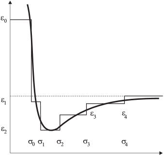
Figure 1: Multistep potential of interactin with parameters $n^{*}=1$, $m^{*}=3$.

Going similarly to the derivation of the kinetic equation of the RET theory [7, 8, 24] and taking into account the system of attractive and repulsive walls, one obtains the following kinetic equation:

$$\left(\frac{\partial}{\partial t}+\vec{v}_{1}\frac{\partial}{\partial\vec{r}_{1}}\right)f_{1}(x_{1};t) = \int\mbox{\rm d}x_{2}\;\hat{T}f_{2}(x_{1},x_{2};t),$$ (2.6)

$$f_{2}(x_{1},x_{2};t) = \text{g}_{2}^{\mathrm{q}}\Big{(}\vec{r}_{1},\vec{r}_{2}|n(t),\beta(t)\Big{)}f_{1}(x_{1};t)f_{1}(x_{2};t),$$

where $\text{g}_{2}^{\mathrm{q}}\Big{(}\vec{r}_{1},\vec{r}_{2}|n(t),\beta(t)\Big{)}$ is defined in the usual way from maximum of the entropy functional and in its turn is the functional of local values of density $n(\vec{r}_{1};t)$ and temperature $\beta(\vec{r}_{1};t)$. $\hat{T}$ is an operator which describes interaction of two particles at presence of MSPI:

$$\hat{T} = \hat{T}_{\mathrm{hs}}^{a}+\sum_{i=1}^{n^{*}}\hat{T}_{li}+\sum_{j=1}^{m^{*}}\hat{T}_{rj},$$ (2.7)

$$\hat{T}_{\mathrm{hs}}^{a} = \sigma_{0}^{2}\int\mbox{\rm d}\hat{\sigma}\;\hat{\sigma}\text{\bf g}\;\theta(\hat{\sigma}\text{\bf g})\left\{\delta\left(\vec{r}_{1}-\vec{r}_{2}+\hat{\sigma}\sigma_{0}^{+}\right)B_{a}(\hat{\sigma})-\delta\left(\vec{r}_{1}-\vec{r}_{2}-\hat{\sigma}\sigma_{0}^{+}\right)\right\}.$$

The last expression is nothing but operator of hard spheres interaction [25], $\hat{\sigma}$ is the unit vector along distance from the second particle to the first one, $\text{\bf g}=\vec{v}_{2}-\vec{v}_{1}$ is relative velocity. $B_{a}(\hat{\sigma})$ is the velocities shift operator as in classical mechanics of elastic collisions. $\hat{T}_{li}=\sum_{k=b,c,d}\hat{T}_{lik}$ is an interaction operator on $i$th repulsive wall; $\hat{T}_{rj}=\sum_{k=b,c,d}\hat{T}_{rjk}$ is an interaction operator on $j$th attractive wall; $a$, $b$, $c$ are types of possible interactions (see Fig. 2).

Figure 2: Types of possible interactions (schematic draw).

$$\hat{T}_{{li\atop rj}k}=\sigma_{{li\atop rj}}^{2}\int\mbox{\rm d}\hat{\sigma}\;\hat{\sigma}\text{\bf g}\;\theta_{{li\atop rj}k}(\ldots)\times{}$$ (2.9)

$$\left\{\delta\left(\vec{r}_{1}-\vec{r}_{2}+\hat{\sigma}\sigma_{{li\atop rj}}^{+}\right)B_{{li\atop rj}k}(\hat{\sigma})-\delta\left(\vec{r}_{1}-\vec{r}_{2}-\hat{\sigma}\sigma_{{li\atop rj}}^{+}\right)\right\},$$

where

$$\begin{array}[]{lclclcl}\theta_{lib}&\equiv&\theta(-\hat{\sigma}\text{\bf g}),&&\theta_{rjb}&\equiv&\theta(-\hat{\sigma}\text{\bf g}),\\ \theta_{lic}&\equiv&\displaystyle\theta\left(\hat{\sigma}\text{\bf g}-\frac{4\!\vartriangle\!\!\varepsilon_{li}}{m}\right),&&\theta_{rjc}&\equiv&\displaystyle\theta\left(-\hat{\sigma}\text{\bf g}-\frac{4\!\vartriangle\!\!\varepsilon_{rj}}{m}\right),\\ \theta_{lid}&\equiv&\displaystyle\theta\left(\frac{4\!\vartriangle\!\!\varepsilon_{li}}{m}-\hat{\sigma}\text{\bf g}\right)\theta(\hat{\sigma}\text{\bf g}),&&\theta_{rjd}&\equiv&\displaystyle\theta\left(\frac{4\!\vartriangle\!\!\varepsilon_{li}}{m}+\hat{\sigma}\text{\bf g}\right)\theta(-\hat{\sigma}\text{\bf g}).\end{array}$$ (2.13)

Expressions (2.13) are nothing but conditions for specific type of interaction ($\theta(z)$ is the Heaviside unit step function).

$B_{{li\atop rj}k}(\hat{\sigma})$ is an operator which acts on velocities and changes them in accordance with the interaction of specific type on each wall:

$$B_{{li\atop rj}k}(\hat{\sigma})\Psi(\vec{v}_{1},\vec{v}_{2})=\Psi(\vec{v}_{1{l\atop r}k},\vec{v}_{2{l\atop r}k}).$$ (2.14)

Type “$a$”:

$$\begin{array}[]{ll}\vec{v}_{1}^{\prime}&=\vec{v}_{1}+\hat{\sigma}(\hat{\sigma}\text{\bf g});\\ \vec{v}_{2}^{\prime}&=\vec{v}_{1}-\hat{\sigma}(\hat{\sigma}\text{\bf g});\\ \end{array}$$ (2.17)

type “$b$”:

$$\begin{array}[]{ll}\vec{v}_{1l}^{\prime\prime}&\displaystyle=\vec{v}_{1}+\frac{1}{2}\hat{\sigma}\left(\hat{\sigma}\text{\bf g}+\sqrt{(\hat{\sigma}\text{\bf g})^{2}+\frac{4\!\vartriangle\!\!\varepsilon_{li}}{m}}\right);\\[8.61108pt] \vec{v}_{1r}^{\prime\prime}&\displaystyle=\vec{v}_{1}+\frac{1}{2}\hat{\sigma}\left(\hat{\sigma}\text{\bf g}-\sqrt{(\hat{\sigma}\text{\bf g})^{2}+\frac{4\!\vartriangle\!\!\varepsilon_{rj}}{m}}\right);\\ \end{array}$$ (2.20)

type “$c$”:

$$\begin{array}[]{ll}\vec{v}_{1l}^{\prime\prime\prime}&\displaystyle=\vec{v}_{1}+\frac{1}{2}\hat{\sigma}\left(\hat{\sigma}\text{\bf g}-\sqrt{(\hat{\sigma}\text{\bf g})^{2}-\frac{4\!\vartriangle\!\!\varepsilon_{li}}{m}}\right);\\[8.61108pt] \vec{v}_{1r}^{\prime\prime\prime}&\displaystyle=\vec{v}_{1}+\frac{1}{2}\hat{\sigma}\left(\hat{\sigma}\text{\bf g}+\sqrt{(\hat{\sigma}\text{\bf g})^{2}-\frac{4\!\vartriangle\!\!\varepsilon_{rj}}{m}}\right);\\ \end{array}$$ (2.23)

type “$d$”:

$$\vec{v}_{1{l\atop r}}^{\prime\prime\prime}=\vec{v}_{1}+\hat{\sigma}(\hat{\sigma}\text{\bf g})\equiv\vec{v}_{1}^{\prime}.$$ (2.24)

Now kinetic equation (2.6) can be rewritten in an explicit form:

$$\left(\frac{\partial}{\partial t}+\vec{v}_{1}\frac{\partial}{\partial\vec{r}_{1}}\right)f_{1}(x_{1};t)={}$$ (2.25)

$$\sigma_{0}\int\mbox{\rm d}\hat{\sigma}\mbox{\rm d}\vec{v}_{2}\;\hat{\sigma}\text{\bf g}\;\theta(\hat{\sigma}\text{\bf g})\left\{f_{2}(\vec{r}_{1},\vec{v}_{1}^{\prime},\vec{r}_{1}+\hat{\sigma}\sigma_{0}^{+},\vec{v}_{2}^{\prime};t)-f_{2}(x_{1},\vec{r}_{1}-\hat{\sigma}\sigma_{0}^{+},\vec{v}_{2};t)\right\}+{}$$

$$\sum_{i=1}^{n^{*}}\sigma_{li}^{2}\int\mbox{\rm d}\hat{\sigma}\mbox{\rm d}\vec{v}_{2}\;\hat{\sigma}\text{\bf g}\times{}$$

$$\left[\theta(-\hat{\sigma}\text{\bf g})\left\{f_{2}(\vec{r}_{1},\vec{v}_{1l}^{\prime\prime},\vec{r}_{1}+\hat{\sigma}\sigma_{li}^{+},\vec{v}_{2l}^{\prime\prime};t)-f_{2}(x_{1},\vec{r}_{1}-\hat{\sigma}\sigma_{li}^{-},\vec{v}_{2};t)\right\}\right.+{}$$

$$\theta\left(\hat{\sigma}\text{\bf g}-{\displaystyle\sqrt{\frac{4\!\vartriangle\!\!\varepsilon_{li}}{m}}}\right)\left\{f_{2}(\vec{r}_{1},\vec{v}_{1l}^{\prime\prime\prime},\vec{r}_{1}+\hat{\sigma}\sigma_{li}^{-},\vec{v}_{2l}^{\prime\prime\prime};t)-f_{2}(x_{1},\vec{r}_{1}-\hat{\sigma}\sigma_{li}^{+},\vec{v}_{2};t)\right\}+{}$$

$$\theta(\hat{\sigma}\text{\bf g})\theta\left({\displaystyle\sqrt{\frac{4\!\vartriangle\!\!\varepsilon_{li}}{m}}}-\hat{\sigma}\text{\bf g}\right)\times{}$$

$$\left.\left\{f_{2}(\vec{r}_{1},\vec{v}_{1l}^{\prime\prime\prime\prime},\vec{r}_{1}+\hat{\sigma}\sigma_{li}^{+},\vec{v}_{2l}^{\prime\prime\prime\prime};t)-f_{2}(x_{1},\vec{r}_{1}-\hat{\sigma}\sigma_{li}^{+},\vec{v}_{2};t)\right\}\right]+{}$$

$$\sum_{j=1}^{m^{*}}\sigma_{rj}^{2}\int\mbox{\rm d}\hat{\sigma}\mbox{\rm d}\vec{v}_{2}\;\hat{\sigma}\text{\bf g}\times{}$$

$$\left[\theta(\hat{\sigma}\text{\bf g})\left\{f_{2}(\vec{r}_{1},\vec{v}_{1r}^{\prime\prime},\vec{r}_{1}+\hat{\sigma}\sigma_{rj}^{-},\vec{v}_{2r}^{\prime\prime};t)-f_{2}(x_{1},\vec{r}_{1}-\hat{\sigma}\sigma_{rj}^{+},\vec{v}_{2};t)\right\}\right.+{}$$

$$\theta\left(-\hat{\sigma}\text{\bf g}-{\displaystyle\sqrt{\frac{4\!\vartriangle\!\!\varepsilon_{rj}}{m}}}\right)\times{}$$

$$\left\{f_{2}(\vec{r}_{1},\vec{v}_{1r}^{\prime\prime\prime},\vec{r}_{1}+\hat{\sigma}\sigma_{rj}^{+},\vec{v}_{2r}^{\prime\prime\prime};t)-f_{2}(x_{1},\vec{r}_{1}-\hat{\sigma}\sigma_{rj}^{-},\vec{v}_{2};t)\right\}+{}$$

$$\theta(-\hat{\sigma}\text{\bf g})\theta\left({\displaystyle\sqrt{\frac{4\!\vartriangle\!\!\varepsilon_{rj}}{m}}}+\hat{\sigma}\text{\bf g}\right)\times{}$$

$$\left.\left\{f_{2}(\vec{r}_{1},\vec{v}_{1r}^{\prime\prime\prime\prime},\vec{r}_{1}+\hat{\sigma}\sigma_{rj}^{-},\vec{v}_{2r}^{\prime\prime\prime\prime};t)-f_{2}(x_{1},\vec{r}_{1}-\hat{\sigma}\sigma_{rj}^{-},\vec{v}_{2};t)\right\}\right]={}$$

$$J_{\mathrm{E}}(f_{1},f_{1})+\sum_{i=1}^{n^{*}}\left(J_{lib}+J_{lic}+J_{lid}\right)+\sum_{j=1}^{m^{*}}\left(J_{rjb}+J_{rjc}+J_{rjd}\right)$$.

One can draw the following conclusions regarding the form of (2.25). In the absence of attractive and repulsive walls ($\!\vartriangle\!\!\varepsilon_{li}=0$, $i=1,\ldots,n^{*}$, $\!\vartriangle\!\!\varepsilon_{rj}=0$, $j=1,\ldots,m^{*}$) this kinetic equation transfers to that one of the RET theory [7, 8]. In the presence of only one finite attractive wall ($\!\vartriangle\!\!\varepsilon_{li}=0$, $i=1,\ldots,n^{*}$, $\!\vartriangle\!\!\varepsilon_{rj}=0$, $j=2,\ldots,m^{*}$, $\!\vartriangle\!\!\varepsilon_{r1}\neq 0$) one obtains the kinetic equation of the RDRS theory [9]. Moreover, it can be shown, in the third special case when the set of walls is merged with some smooth potential $\phi_{t}$ and $\!\vartriangle\!\!\sigma_{li}=\sigma_{li}-\sigma_{li-1}\to 0$, $i=1,\ldots,n^{*}-1$, $\!\vartriangle\!\!\varepsilon_{li}\to 0$, $n^{*}\to\infty$, $\!\vartriangle\!\!\sigma_{rj}=\sigma_{rj+1}-\sigma_{rj}\to 0$, $j=1,\ldots,m^{*}-1$, $\!\vartriangle\!\!\varepsilon_{rj}\to 0$, $m^{*}\to\infty$, and

$$-\frac{\!\vartriangle\!\!\varepsilon_{li}}{\!\vartriangle\!\!\sigma_{li}} \to \phi^{\prime}_{t}(\sigma_{li}),$$

$$\frac{\!\vartriangle\!\!\varepsilon_{rj}}{\!\vartriangle\!\!\sigma_{rj}} \to \phi^{\prime}_{t}(\sigma_{rj}),$$

kinetic equation (2.25) transfers to those one of the KMFT theory [19].

3 Macroscopic conservation laws. The zeroth approximation

Let us introduce the following set of hydrodynamic parameters: particles number density $n(\vec{r};t)$, hydrodynamic velocity $\vec{u}(\vec{r};t)$, densities of kinetic $\omega_{\mathrm{k}}$ and interaction $\omega_{\mathrm{i}}$ energies:

$$\begin{array}[]{rcl}n(\vec{r}_{1};t)&=&\displaystyle\int\mbox{\rm d}\vec{v}_{2}\;f_{1}(x_{1};t),\\ \vec{u}(\vec{r}_{1};t)&=&\displaystyle\int\mbox{\rm d}\vec{v}_{2}\;f_{1}(x_{1};t)\frac{\vec{v}_{1}}{n(\vec{r}_{1};t)},\\[4.30554pt] \omega_{\mathrm{k}}(\vec{r}_{1};t)&=&\displaystyle\int\mbox{\rm d}\vec{v}_{2}\;f_{1}(x_{1};t)\frac{c_{1}^{2}}{2n(\vec{r}_{1};t)},\\ \omega_{\mathrm{i}}(\vec{r}_{1};t)&=&\displaystyle\int\mbox{\rm d}\vec{r}_{2}\;n(\vec{r}_{2};t)\text{g}_{2}^{\mathrm{q}}(\vec{r}_{1},\vec{r}_{2}|n(t),\beta(t))\frac{1}{2m}\Phi(|\vec{r}_{12}|).\\ \end{array}$$ (3.5)

We also introduce the set of interaction invariants $\vec{\Psi}$$\equiv$$\left\{\!m,m\vec{v},\frac{1}{2}\!\left[mv^{2}\mbox{+}\phi(r_{12})\right]\!\right\}$. Multiplying initial kinetic equation (2.25) on each component of the vector $\vec{\Psi}$ and integrating with respect to $\vec{v}_{2}$ one obtains the equation of continuity, the equation of motion and equation of balance of kinetic energy, correspondingly:

$$\begin{array}[]{rcl}\displaystyle\frac{1}{n}\frac{\mbox{\rm d}n}{\mbox{\rm d}t}&=&\displaystyle-\frac{\partial}{\partial r_{1\alpha}}u_{\alpha},\\ \displaystyle\frac{\mbox{\rm d}u_{\alpha}}{\mbox{\rm d}t}&=&\displaystyle-\frac{1}{mn}\frac{\partial}{\partial r_{1\beta}}P_{\alpha\beta},\\ \displaystyle\frac{\mbox{\rm d}\omega_{\mathrm{k}}}{\mbox{\rm d}t}&=&\displaystyle-\frac{1}{mn}\left\{\frac{\partial}{\partial r_{1\alpha}}q_{\alpha}+P_{\alpha\beta}\frac{\partial}{\partial r_{1\beta}}u_{\alpha}\right\},\\ \end{array}\quad\frac{\mbox{\rm d}}{\mbox{\rm d}t}=\frac{\partial}{\partial t}+u_{\gamma}\frac{\partial}{\partial r_{1\gamma}}.$$ (3.9)

The equation for interaction energy density one obtains automatically differentiating the expression for $\omega_{\mathrm{i}}$ taking into account conservation laws for $n(\vec{r};t)$, $\vec{u}(\vec{r};t)$ and $\omega_{\mathrm{k}}$ (3.9). Stress tensor $P_{\alpha\beta}$ and heat flow vector consist on kinetic and interaction parts:

$$\begin{array}[]{lclcll}P_{\alpha\beta}&=&P_{\alpha\beta}^{\mathrm{k}}&+&P_{\alpha\beta}^{\mathrm{i}}&,\\ q_{\alpha}&=&q_{\alpha}^{\mathrm{k}}&+&q_{\alpha}^{\mathrm{i}}&.\\ \end{array}$$ (3.12)

In its turn, the potential parts consist of the hard sphere term and components conditioned by the set of attractive and repulsive walls:

$$\begin{array}[]{llllllllllll}P_{\alpha\beta}^{\mathrm{i}}&=P_{1\alpha\beta}^{\mathrm{i}}&+\!\displaystyle\sum_{i=1}^{n^{*}}(P_{i2\alpha\beta}^{\mathrm{i}}&+&P_{i3\alpha\beta}^{\mathrm{i}}&+&P_{i4\alpha\beta}^{\mathrm{i}})&+\displaystyle\sum_{j=1}^{m^{*}}(P_{j2\alpha\beta}^{\mathrm{i}}&+&P_{j3\alpha\beta}^{\mathrm{i}}&+&P_{j4\alpha\beta}^{\mathrm{i}}),\\ q_{\alpha}^{\mathrm{i}}&=q_{1\alpha}^{\mathrm{i}}&+\!\displaystyle\sum_{i=1}^{n^{*}}(q_{i2\alpha}^{\mathrm{i}}&+&q_{i3\alpha}^{\mathrm{i}}&+&q_{i4\alpha}^{\mathrm{i}})&+\displaystyle\sum_{j=1}^{m^{*}}(q_{j2\alpha}^{\mathrm{i}}&+&q_{j3\alpha}^{\mathrm{i}}&+&q_{j4\alpha}^{\mathrm{i}}),\\ \end{array}$$ (3.15)

(3.16)

where indices 1, 2, 3, and 4 correspond to different types of interactions: “$a$”, “$b$”, “$c$”, and “$d$”, correspondingly. Now let us write down the expressions for stress tensor $P_{\alpha\beta}$ and heat flow vector $q_{\alpha}$ in an explicit form:

$$\begin{array}[]{ll}P_{\alpha\beta}^{\mathrm{k}}&=\displaystyle\int\mbox{\rm d}\vec{v}_{1}\;f_{1}(x_{1};t)mc_{1\alpha}c_{1\beta},\\ q_{\alpha}^{\mathrm{k}}&=\displaystyle\int\mbox{\rm d}\vec{v}_{1}\;f_{1}(x_{1};t)\frac{mc_{1}^{2}}{2}c_{1\alpha},\\ \end{array}$$ (3.19)

$$P_{1\alpha\beta}^{\mathrm{i}} = \frac{1}{2}m\sigma_{0}^{3}\int\mbox{\rm d}\vec{v}_{1}\mbox{\rm d}\vec{v}_{2}\mbox{\rm d}\hat{\sigma}\;\hat{\sigma}\text{\bf g}\;\theta(\hat{\sigma}\text{\bf g})\left(v_{1\alpha}^{\prime}-v_{1\alpha}\right)\hat{\sigma}_{\beta}\times{}$$

$$\int_{0}^{1}\mbox{\rm d}\lambda\;f_{2}(\vec{r}_{1}+\lambda\hat{\sigma}\sigma_{0}^{+},\vec{v}_{1},\vec{r}_{1}+\lambda\hat{\sigma}\sigma_{0}^{+}-\hat{\sigma}\sigma_{0}^{+},\vec{v}_{2};t),$$

$$q_{1\alpha}^{\mathrm{i}} = \frac{1}{2}m\sigma_{0}^{3}\int\mbox{\rm d}\vec{v}_{1}\mbox{\rm d}\vec{v}_{2}\mbox{\rm d}\hat{\sigma}\;\hat{\sigma}\text{\bf g}\;\theta(\hat{\sigma}\text{\bf g})\left(\frac{\left(c_{1}^{\prime}\right)^{2}}{2}-\frac{c_{1}^{2}}{2}\right)\hat{\sigma}_{\alpha}\times{}$$

$$\int_{0}^{1}\mbox{\rm d}\lambda\;f_{2}(\vec{r}_{1}+\lambda\hat{\sigma}\sigma_{0}^{+},\vec{v}_{1},\vec{r}_{1}+\lambda\hat{\sigma}\sigma_{0}^{+}-\hat{\sigma}\sigma_{0}^{+},\vec{v}_{2};t),$$

$$P_{i2\alpha\beta}^{\mathrm{i}} = \frac{1}{2}m\sigma_{li}^{3}\int\mbox{\rm d}\vec{v}_{1}\mbox{\rm d}\vec{v}_{2}\mbox{\rm d}\hat{\sigma}\;\hat{\sigma}\text{\bf g}\;\theta(-\hat{\sigma}\text{\bf g})\left(v_{1l\alpha}^{\prime\prime}-v_{1\alpha}\right)\hat{\sigma}_{\beta}\times{}$$

$$\int_{0}^{1}\mbox{\rm d}\lambda\;f_{2}(\vec{r}_{1}+\lambda\hat{\sigma}\sigma_{li}^{-},\vec{v}_{1},\vec{r}_{1}+\lambda\hat{\sigma}\sigma_{li}^{-}-\hat{\sigma}\sigma_{li}^{-},\vec{v}_{2};t),$$

$$q_{i2\alpha}^{\mathrm{i}} = \frac{1}{2}m\sigma_{li}^{3}\int\mbox{\rm d}\vec{v}_{1}\mbox{\rm d}\vec{v}_{2}\mbox{\rm d}\hat{\sigma}\;\hat{\sigma}\text{\bf g}\;\theta(-\hat{\sigma}\text{\bf g})\left(\frac{\left(c_{1l}^{\prime\prime}\right)^{2}}{2}-\frac{c_{1}^{2}}{2}-\frac{\!\vartriangle\!\!\varepsilon_{li}}{m}\right)\hat{\sigma}_{\alpha}\times{}$$

$$\int_{0}^{1}\mbox{\rm d}\lambda\;f_{2}(\vec{r}_{1}+\lambda\hat{\sigma}\sigma_{li}^{-},\vec{v}_{1},\vec{r}_{1}+\lambda\hat{\sigma}\sigma_{li}^{-}-\hat{\sigma}\sigma_{li}^{-},\vec{v}_{2};t),$$

$$P_{i3\alpha\beta}^{\mathrm{i}} = \frac{1}{2}m\sigma_{li}^{3}\int\mbox{\rm d}\vec{v}_{1}\mbox{\rm d}\vec{v}_{2}\mbox{\rm d}\hat{\sigma}\;\hat{\sigma}\text{\bf g}\;\theta\left(\hat{\sigma}\text{\bf g}-\sqrt{\frac{4\!\vartriangle\!\!\varepsilon_{li}}{m}}\right)\left(v_{1l\alpha}^{\prime\prime\prime}-v_{1\alpha}\right)\hat{\sigma}_{\beta}\times{}$$

$$\int_{0}^{1}\mbox{\rm d}\lambda\;f_{2}(\vec{r}_{1}+\lambda\hat{\sigma}\sigma_{li}^{+},\vec{v}_{1},\vec{r}_{1}+\lambda\hat{\sigma}\sigma_{li}^{+}-\hat{\sigma}\sigma_{li}^{+},\vec{v}_{2};t),$$

$$q_{i3\alpha}^{\mathrm{i}} = \frac{1}{2}m\sigma_{li}^{3}\int\mbox{\rm d}\vec{v}_{1}\mbox{\rm d}\vec{v}_{2}\mbox{\rm d}\hat{\sigma}\;\hat{\sigma}\text{\bf g}\;\theta\left(\hat{\sigma}\text{\bf g}-\sqrt{\frac{4\!\vartriangle\!\!\varepsilon_{li}}{m}}\right)\left[\frac{\left(c_{1l}^{\prime\prime\prime}\right)^{2}}{2}-\frac{c_{1}^{2}}{2}+\frac{\!\vartriangle\!\!\varepsilon_{li}}{2m}\right]\hat{\sigma}_{\alpha}$$ (3.25)

$$\times \int_{0}^{1}\mbox{\rm d}\lambda\;f_{2}(\vec{r}_{1}+\lambda\hat{\sigma}\sigma_{li}^{+},\vec{v}_{1},\vec{r}_{1}+\lambda\hat{\sigma}\sigma_{li}^{+}-\hat{\sigma}\sigma_{li}^{+},\vec{v}_{2};t),$$

$$P_{i4\alpha\beta}^{\mathrm{i}} = \frac{1}{2}m\sigma_{li}^{3}\int\mbox{\rm d}\vec{v}_{1}\mbox{\rm d}\vec{v}_{2}\mbox{\rm d}\hat{\sigma}\;\hat{\sigma}\text{\bf g}\;\theta(\hat{\sigma}\text{\bf g})\theta\left(\sqrt{\frac{4\!\vartriangle\!\!\varepsilon_{li}}{m}}-\hat{\sigma}\text{\bf g}\right)\left(v_{1l\alpha}^{\prime\prime\prime\prime}-v_{1\alpha}\right)\hat{\sigma}_{\beta}\times{}$$ (3.26)

$$\int_{0}^{1}\mbox{\rm d}\lambda\;f_{2}(\vec{r}_{1}+\lambda\hat{\sigma}\sigma_{li}^{+},\vec{v}_{1},\vec{r}_{1}+\lambda\hat{\sigma}\sigma_{li}^{+}-\hat{\sigma}\sigma_{li}^{+},\vec{v}_{2};t),$$

$$q_{i4\alpha}^{\mathrm{i}} = \frac{1}{2}m\sigma_{li}^{3}\int\mbox{\rm d}\vec{v}_{1}\mbox{\rm d}\vec{v}_{2}\mbox{\rm d}\hat{\sigma}\;\hat{\sigma}\text{\bf g}\;\theta(\hat{\sigma}\text{\bf g})\theta\left(\sqrt{\frac{4\!\vartriangle\!\!\varepsilon_{li}}{m}}-\hat{\sigma}\text{\bf g}\right)\left(\frac{\left(c_{1l}^{\prime\prime\prime\prime}\right)^{2}}{2}-\frac{c_{1}^{2}}{2}\right)\times{}$$ (3.27)

$$\int_{0}^{1}\mbox{\rm d}\lambda\;f_{2}(\vec{r}_{1}+\lambda\hat{\sigma}\sigma_{li}^{+},\vec{v}_{1},\vec{r}_{1}+\lambda\hat{\sigma}\sigma_{li}^{+}-\hat{\sigma}\sigma_{li}^{+},\vec{v}_{2};t).$$

Expressions for $P_{j2\alpha\beta}$, $P_{j3\alpha\beta}$, $P_{j4\alpha\beta}$, $q_{j2\alpha}$, $q_{j3\alpha}$, and $q_{j4\alpha}$ look similar to (3)–(3.27) $P_{i2\alpha\beta}$, $P_{i3\alpha\beta}$, $P_{i4\alpha\beta}$, $q_{i2\alpha}$, $q_{i3\alpha}$, and $q_{ij4\alpha}$, correspondingly, at formal replacing $\sigma_{li}^{\pm}\to\sigma_{rj}^{\mp}$, $\hat{\sigma}\text{\bf g}\to-\hat{\sigma}\text{\bf g}$, $\vec{v}_{1l}\to\vec{v}_{1r}$, $\!\vartriangle\!\!\varepsilon_{li}\to\;\!\vartriangle\!\!\varepsilon_{rj}$.

At the end of this section we consider macroscopic conservation laws in the zeroth approximation. Let us suppose that one-particle distribution function in this case is equal to the local-equilibrium Maxwell one:

$$f_{1}\equiv f_{1}^{(0)}(x_{1};t)=n(\vec{r}_{1};t)\left(\frac{m}{2\pi k_{\rm B}T(\vec{r}_{1};t)}\right)^{\scriptstyle 3/2}\!\!\!\exp\left\{-\frac{mc_{1}^{2}(\vec{r}_{1};t)}{2k_{\rm B}T(\vec{r}_{1};t)}\right\}.$$ (3.28)

Neglecting by any spatial gradients one obtains

$$\text{g}_{2}^{\mathrm{q}}(\vec{r}_{1},\vec{r}_{2}|n(\vec{r}_{1};t),\beta(\vec{r}_{1};t))\simeq\text{g}_{2}^{\mathrm{eq}}\left(r_{12};n\left(\frac{\vec{r}_{1}+\vec{r}_{2}}{2};t\right),\beta\left(\frac{\vec{r}_{1}+\vec{r}_{2}}{2};t\right)\right),$$

(3.29)

$$\int_{0}^{1}\mbox{\rm d}\lambda\;f_{2}(x_{1},x_{2};t)\simeq\displaystyle\int_{0}^{1}\mbox{\rm d}\lambda\;f_{2}^{(0)}(\ldots)=\text{g}_{2}^{\mathrm{eq}}(\sigma|n,\beta)f_{1}^{(0)}(x_{1};t)f_{1}^{(0)}(\vec{r}_{1},\vec{v}_{2};t).$$

It is well known from the equilibrium statistical mechanics [26] that any sharp jump of interaction potential results in a corresponding jump of binary correlation function:

$$\frac{\text{g}_{2}^{\mathrm{eq}}(\sigma_{li}^{+}|n,\beta)}{\text{g}_{2}^{\mathrm{eq}}(\sigma_{li}^{-}|n,\beta)} = \exp\left\{\beta\!\vartriangle\!\!\varepsilon_{li}\right\},$$

$$\frac{\text{g}_{2}^{\mathrm{eq}}(\sigma_{rj}^{-}|n,\beta)}{\text{g}_{2}^{\mathrm{eq}}(\sigma_{rj}^{+}|n,\beta)} = \exp\left\{\beta\!\vartriangle\!\!\varepsilon_{rj}\right\}.$$

Substituting these relations into (3.19)–(3.27), one obtains: $P_{\alpha\beta}=p\delta_{\alpha\beta}$, where $p$ is the hydrostatic pressure which consists on kinetic $p^{\mathrm{k}}$ and interaction $p^{\mathrm{i}}$ parts; $q_{\alpha}=0$:

$$\begin{array}[]{lcl}p&=&p^{\mathrm{k}}+p^{\mathrm{i}},\\ p^{\mathrm{k}}&=&nk_{\rm B}T,\\ p^{\mathrm{i}}&=&\displaystyle\frac{2}{3}\pi n^{2}k_{\rm B}T\Lambda,\\ \Lambda&=&\text{\small$\displaystyle\sigma_{0}^{3}\text{g}_{2}(\sigma_{0}^{+})-\sum_{i=1}^{n^{*}}\sigma_{li}^{3}\text{g}_{2}(\sigma_{li}^{+})\left\{\e^{-\beta\vartriangle\varepsilon_{li}}-1\right\}+\displaystyle\sum_{j=1}^{m^{*}}\sigma_{rj}^{3}\text{g}_{2}(\sigma_{rj}^{-})\left\{\e^{-\beta\vartriangle\varepsilon_{rj}}-1\right\}$}\!,\\ \text{g}_{2}^{\mathrm{eq}}&\equiv&\text{g}_{2}^{\mathrm{eq}}\Big{(}\sigma|n(\vec{r}_{1};t),\beta(\vec{r}_{1};t)\Big{)}.\\ \end{array}$$ (3.36)

Then, starting from (3.9), one has the conservation laws in the zeroth approximation (Euler laws):

$$\begin{array}[]{rcl}\displaystyle\frac{1}{n}\frac{\mbox{\rm d}n}{\mbox{\rm d}t}&=&\displaystyle-\frac{\partial\vec{u}}{\partial\vec{r}_{1}},\\[4.30554pt] \displaystyle\frac{\mbox{\rm d}\vec{u}}{\mbox{\rm d}t}&=&\displaystyle-\frac{1}{mn}\frac{\partial P}{\partial\vec{r}_{1}},\\[4.30554pt] \displaystyle\frac{\mbox{\rm d}\omega_{\mathrm{k}}}{\mbox{\rm d}t}&=&\displaystyle-\frac{1}{mn}p\frac{\partial\vec{u}}{\partial\vec{r}_{1}},\quad\omega_{\mathrm{k}}=\frac{3}{2m\beta},\\[4.30554pt] \omega_{\mathrm{i}}^{(0)}(\vec{r}_{1};t)&=&\displaystyle\frac{1}{2m}\int\mbox{\rm d}\vec{r}_{12}\;n(\vec{r}_{1};t)\text{g}_{2}^{\mathrm{eq}}\Big{(}|\vec{r}_{12}|;n(\vec{r}_{1};t),\beta(\vec{r}_{1};t)\Big{)}\Phi(|\vec{r}_{12}|).\\ \end{array}$$ (3.41)

4 The principle of construction of higher order approximations. Normal solutions by means of boundary conditions method

Let us consider initial kinetic equation (2.6) (or (2.25))

$$\left(\frac{\partial}{\partial t}+\vec{v}_{1}\frac{\partial}{\partial\vec{r}_{1}}\right)f_{1}(x_{1};t)=\int\mbox{\rm d}x_{2}\;\hat{T}f_{2}(x_{1},x_{2};t)=J(f_{1},f_{1}),$$ (4.1)

where the collision integral $J(f_{1},f_{1})$ consists of the usual one of the RET theory – $J_{\mathrm{E}}(f_{1},f_{1})$ and collision integrals demanding on interaction on each wall. Such a structure of $J(f_{1},f_{1})$ is caused by the structure of $\hat{T}$-operator:

$$J(f_{1},f_{1})=J_{\mathrm{E}}(f_{1},f_{1})+\sum_{i=1}^{n^{*}}[J_{lib}+J_{lic}+J_{lid}]+\sum_{j=1}^{m^{*}}[J_{rjb}+J_{rjc}+J_{rjd}].$$ (4.2)

Going to the schema of construction of normal solutions to kinetic equations with the help of boundary conditions [22], let us introduce in the right-hand side of (4.1) an infinitely small source $-\bar{\varepsilon}(f_{1}-f_{1}^{(0)})$, where $\bar{\varepsilon}\to 0$:

$$\left(\frac{\partial}{\partial t}+\vec{v}_{1}\frac{\partial}{\partial\vec{r}_{1}}\right)f_{1}(x_{1};t)=J(f_{1},f_{1})-\bar{\varepsilon}\left(f_{1}-f_{1}^{(0)}\right).$$ (4.3)

For deviation $\delta f=f_{1}-f_{1}^{(0)}$ this equation reads:

$$\left(\frac{\partial}{\partial t}+\vec{v}_{1}\frac{\partial}{\partial\vec{r}_{1}}+\bar{\varepsilon}\right)\delta f=-\left(\frac{\partial}{\partial t}+\vec{v}_{1}\frac{\partial}{\partial\vec{r}_{1}}\right)f_{1}^{(0)}+{}$$ (4.4)

$$J\left(f_{1}^{(0)},f_{1}^{(0)}\right)+J\left(f_{1}^{(0)},\delta f\right)+J\left(\delta f,f_{1}^{(0)}\right)+J\left(\delta f,\delta f\right).$$

First and foremost it should be noted that in the collision integral in the usual Boltzmann equation is local ($f_{1}$ is a function of the same Cartesian coordinate $\vec{r}_{1}$). In our case the $J(f_{1},f_{1})$ is a nonlocal collision integral. One time $f_{1}$ is calculated in $\vec{r}_{1}$, second time – in $\vec{r}_{1}\pm\hat{\sigma}\sigma$, integration with respect to $\hat{\sigma}$ (surface of unit sphere) is performed. As a consequence of that in one or another way we will find solutions in some approximation and there is no sense “to draw” the whole nonlocal collision integral. It is much convenient to use its approximate expression. This approximation should be the same order as within the frame for the solution of total kinetic equation. In such a way, let us expand functions $f_{1}$ and $\text{g}_{2}^{\mathrm{q}}$ in the vicinity of $\vec{r}_{1}$ into series on deviations $\pm\hat{\sigma}\sigma$. This results in:

$$\displaystyle J\equiv\sum_{k=0}^{\infty}J_{k}=J_{0}+J^{*},$$ J^*=∑_k=1^∞J_k, (4.5)

$$\displaystyle I\equiv\sum_{k=0}^{\infty}I_{k}=I_{0}+I^{*},$$ I^*=∑_k=1^∞I_k, (4.6)

where $k$ is the expansion order. All $J_{k}$ are here local functionals of $f_{1}$. We also use the following notations: $I(\delta f)=J\left(f_{1}^{(0)},\delta f\right)+J\left(\delta f,f_{1}^{(0)}\right)$ – linearized nonlocal collision operator. We have similar expansion for this operator – the relation (4.6). Here $I_{0}(\delta f)=J_{0}\left(f_{1}^{(0)},\delta f\right)+J_{0}\left(\delta f,f_{1}^{(0)}\right)$ is linearized local collision operator which coincides with those one of the usual Boltzmann kinetic equation within a factor of $\text{g}_{2}^{\mathrm{eq}}(\sigma_{0}^{+})$ if one neglects the set of walls except hard sphere wall only. Then equation (4.4) transfers to

$$\frac{\partial}{\partial t}\delta f+\bar{\varepsilon}\delta f-I_{0}(\delta f)={}$$ (4.7)

$$-\frac{\mathrm{D}}{\mathrm{D}t}f_{1}^{(0)}+J\left(f_{1}^{(0)},f_{1}^{(0)}\right)+I^{*}(\delta f)+J(\delta f,\delta f)-\vec{v}_{1}\frac{\partial}{\partial\vec{r}_{1}}\delta f.$$

To solve this equation by means the boundary conditions method we need in its integral form. To this end let us introduce operator $S(t,t^{\prime})$ with the following properties:

$$\frac{\partial}{\partial t}S(t,t^{\prime})=I_{0}S(t,t^{\prime}),\quad S(t,t)=1.$$ (4.8)

Using the limiting condition $\displaystyle\lim_{t\to-\infty}\delta f(t)=0$ one obtains:

$$\delta f(t) = \int_{-\infty}^{t}\mbox{\rm d}t^{\prime}\;\e^{\bar{\varepsilon}(t^{\prime}-t)}S(t,t^{\prime})\times{}$$

$$\left[\frac{\mathrm{D}}{\mathrm{D}t}f_{1}^{(0)}+J\left(f_{1}^{(0)},f_{1}^{(0)}\right)+I^{*}(\delta f)+J(\delta f,\delta f)-\vec{v}_{1}\frac{\partial}{\partial\vec{r}_{1}}\delta f\right]_{t^{\prime}}.$$

Equation (4) is completely ready for iteration procedure. This procedure can be organized as follows:

$$\delta f^{(k+1)}(t) = \int_{-\infty}^{t}\mbox{\rm d}t^{\prime}\;\e^{\bar{\varepsilon}(t^{\prime}-t)}S(t,t^{\prime})\left[\frac{\mathrm{D}}{\mathrm{D}t}f_{1}^{(0)}+J^{(k+1)}\left(f_{1}^{(0)},f_{1}^{(0)}\right)+{}\right.$$

$$\left.I^{*(k+1)}\left(\delta f^{(k)}\right)+J^{(k+1)}\left(\delta f^{(k)},\delta f^{(k)}\right)-\vec{v}_{1}\frac{\partial}{\partial\vec{r}_{1}}\delta f^{(k)}\right]_{t^{\prime}},$$

where

$$J^{(k+1)} = \sum_{k^{\prime}=0}^{k+1}J_{k^{\prime}},$$

$$I^{*(k+1)} = \sum_{k^{\prime}=0}^{k+1}I_{k^{\prime}}.$$

Each $(k+1)$th step uses conservation laws in $k$th approximation.

5 Distribution function $\boldsymbol{f_{1}}$ in the first approximation

The expression for distribution function $f_{1}$ in the first approximation is obtained if one puts into (3.19) $k=0$ and take into account the equality $\delta f^{(0)}=0$. Then we have:

$$\delta f^{(1)}(t) = \!\int_{-\infty}^{t}\mbox{\rm d}t^{\prime}\;\e^{\varepsilon(t^{\prime}-t)}S(t,t^{\prime})\!\left[\frac{\mathrm{D}}{\mathrm{D}t}f_{1}^{(0)}+J_{0}\left(f_{1}^{(0)},f_{1}^{(0)}\right)+J_{1}\left(f_{1}^{(0)},f_{1}^{(0)}\right)\right]_{t^{\prime}}.$$

It can be shown that

$$J_{0}\left(f_{1}^{(0)},f_{1}^{(0)}\right)=0.$$ (5.2)

Making the expansion with an accuracy of first order on gradients of hydrodynamic parameters

$$\text{g}_{2}^{\mathrm{q}}(\vec{r}_{1},\vec{r}_{2}|n(t),\beta(t)) \simeq \text{g}_{2}^{\mathrm{eq}}\left(r_{12};n\left(\frac{\vec{r}_{1}+\vec{r}_{2}}{2};t\right),\beta\left(\frac{\vec{r}_{1}+\vec{r}_{2}}{2};t\right)\right)$$ (5.3)

$$= \frac{1}{2}\vec{r}_{12}\frac{\partial}{\partial\vec{r}_{1}}\text{g}_{2}^{\mathrm{eq}}+\ldots,$$

$$f_{1}(\vec{r}_{1}\pm\hat{\sigma}\sigma) = f_{1}(\vec{r}_{1})\pm\frac{\partial}{\partial\vec{r}_{1}}f_{1}\;\hat{\sigma}\sigma+\ldots$$

and taking into consideration conservation laws (3.41) one obtains after very unwieldy calculations the following:

$$-\frac{\mathrm{D}}{\mathrm{D}}f_{1}^{(0)}+J_{1}\left(f_{1}^{(0)},f_{1}^{(0)}\right)=K_{\alpha}\frac{\partial}{\partial r_{1\alpha}}\ln T+L_{\alpha\beta}\frac{\partial}{\partial r_{1\beta}}u_{\alpha},$$ (5.4)

$$K_{\alpha}$$L_αβ = -f_1^(0)[1+35pinkBT][mc122kBT-52]c_1α+ ∑_i=1^n^*K_αli+∑_j=1^m^*K_αrj, (5.5)

$$L_{\alpha\beta}$$L_αβ = -f_1^(0) [1+25pinkBT]mkBT[c_1αc_1β-13c_1^2δ_αβ]+ ∑_i=1^n^*L_αβli+∑_j=1^m^*L_αβrj,

where

$$K_{\alpha{li\atop rj}} = \mp\frac{8}{\pi^{2}}n^{2}\sigma_{{li\atop rj}}\text{g}_{2}^{\mathrm{eq}}\left(\sigma_{li\atop rj}^{\pm}\right)\frac{m}{2k_{\rm B}T}\times{}$$

$$\left[\frac{1}{30}\e^{-s^{2}}\int\mbox{\rm d}\vec{x}_{2}\;\exp\left\{-h^{2}-v^{2}\right\}h_{\beta}\left(v_{\alpha}v_{\beta}-\frac{1}{3}v^{2}\delta_{\alpha\beta}\right)\times{}\right.$$

$$\phantom{\bigg{[}}\left\{4+\frac{s^{3}}{v^{5}}\left(5v^{2}+6s^{2}\right)+\frac{1}{v^{5}}\left(v^{2}+s^{2}\right)^{3/2}\left(4v^{2}-6s^{2}\right)\right\}-{}$$

$$\phantom{\bigg{[}}\frac{1}{30}\int_{v>s}\mbox{\rm d}\vec{x}_{2}\;\exp\left\{-h^{2}-v^{2}\right\}h_{\beta}\left(v_{\alpha}v_{\beta}-\frac{1}{3}v^{2}\delta_{\alpha\beta}\right)\times{}$$

$$\phantom{\bigg{[}}\left\{4+\frac{s^{3}}{v^{5}}\left(5v^{2}-9s^{2}\right)+\frac{1}{v^{5}}\left(v^{2}-s^{2}\right)^{3/2}\left(4v^{2}+6s^{2}\right)\right\}+{}$$

$$\phantom{\bigg{[}}\frac{1}{9}\e^{-s^{2}}\int\mbox{\rm d}\vec{x}_{2}\;\exp\left\{-h^{2}-v^{2}\right\}h_{\alpha}\left(v^{2}-\frac{s^{3}}{v}+\frac{1}{v}\left(v^{2}+s^{2}\right)^{3/2}\right)-{}$$

$$\phantom{\bigg{[}}\frac{1}{9}\int_{v>s}\left.\mbox{\rm d}\vec{x}_{2}\;\exp\left\{-h^{2}-v^{2}\right\}h_{\alpha}\left(v^{2}-\frac{s^{3}}{v}+\frac{1}{v}\left(v^{2}+s^{2}\right)^{3/2}\right)\right],$$

$$L_{\alpha\beta{li\atop rj}} = \mp\frac{8}{\pi^{2}}n^{2}\sqrt{2}\sigma_{{li\atop rj}}\text{g}_{2}^{\mathrm{eq}}\left(\sigma_{li\atop rj}^{\pm}\right)\left(\frac{m}{2k_{\rm B}T}\right)^{3/2}\times{}$$

$$\left[\frac{1}{30}\e^{-s^{2}}\int\mbox{\rm d}\vec{x}_{2}\;\exp\left\{-h^{2}-v^{2}\right\}\left(v_{\alpha}v_{\beta}-\frac{1}{3}v^{2}\delta_{\alpha\beta}\right)\times{}\right.$$

$$\phantom{\bigg{[}}\left\{4+\frac{s^{3}}{v^{5}}\left(5v^{2}+6s^{2}\right)+\frac{1}{v^{5}}\left(v^{2}+s^{2}\right)^{3/2}\left(4v^{2}-6s^{2}\right)\right\}-{}$$

$$\phantom{\bigg{[}}\frac{1}{30}\int_{v>s}\mbox{\rm d}\vec{x}_{2}\;\exp\left\{-h^{2}-v^{2}\right\}\left(v_{\alpha}v_{\beta}-\frac{1}{3}v^{2}\delta_{\alpha\beta}\right)\times{}$$

$$\phantom{\bigg{[}}\left\{4+\frac{s^{3}}{v^{5}}\left(5v^{2}-9s^{2}\right)+\frac{1}{v^{5}}\left(v^{2}-s^{2}\right)^{3/2}\left(4v^{2}+6s^{2}\right)\right\}+{}$$

$$\phantom{\bigg{[}}\frac{1}{9}\e^{-s^{2}}\int\mbox{\rm d}\vec{x}_{2}\;\exp\left\{-h^{2}-v^{2}\right\}\left(v^{2}-\frac{s^{3}}{v}+\frac{1}{v}\left(v^{2}+s^{2}\right)^{3/2}\right)\delta_{\alpha\beta}-{}$$

$$\phantom{\bigg{[}}\frac{1}{9}\int_{v>s}\left.\mbox{\rm d}\vec{x}_{2}\;\exp\left\{-h^{2}-v^{2}\right\}\left(v^{2}-\frac{s^{3}}{v}+\frac{1}{v}\left(v^{2}+s^{2}\right)^{3/2}\right)\delta_{\alpha\beta}\right].$$

Here

$$s=\left\{\begin{array}[]{l}\left(\beta\!\vartriangle\!\!\varepsilon_{li}\right)^{1/2},\\ \left(\beta\!\vartriangle\!\!\varepsilon_{rj}\right)^{1/2},\\ \end{array}\right.\quad\vec{x}_{2}=\left(\frac{m}{4k_{\rm B}T}\right)^{1/2}\vec{c}_{2},$$ (5.11)

$$\begin{array}[]{lclcl}\displaystyle\vec{v}=\left(\frac{m}{4k_{\rm B}T}\right)^{1/2}\text{\bf g},&&\text{\bf g}&=&\vec{c}_{2}-\vec{c}_{1},\\ \displaystyle\vec{h}=2\left(\frac{m}{4k_{\rm B}T}\right)^{1/2}\vec{G}_{0},&&\vec{G}_{0}&=&\displaystyle\frac{1}{2}(\vec{c}_{1}+\vec{c}_{2}).\\ \end{array}$$ (5.14)

Then

$$f_{1}\equiv f_{1}^{(1)} = f_{1}^{(0)}+\delta f^{(1)},$$ (5.15)

$$\delta f^{(1)}(t) = \int_{-\infty}^{t}\mbox{\rm d}t^{\prime}\;\e^{\varepsilon(t^{\prime}-t)}S(t,t^{\prime})\left\{K_{\alpha}\frac{\partial}{\partial r_{1\alpha}}\ln T+L_{\alpha\beta}\frac{\partial}{\partial r_{1\beta}}u_{\alpha}\right\}_{t^{\prime}}.$$

It can be shown that $\int\mbox{\rm d}\vec{v}_{1}\;\delta f^{(1)}(\vec{r}_{1},\vec{v}_{1};t)\vec{\Psi}=0$, i.e. the hydrodynamic parameters $n(\vec{r}_{1};t)$, $\vec{u}(\vec{r}_{1};t)$, $\beta$, $\omega_{\mathrm{i}}$ are completely defined by the local one-particle distribution function $f_{1}^{(0)}$ (3.28).

6 Conservation laws in the first approximation. Stationary process

First, let us calculate kinetic parts of the stress tensor and heat flux vector. Substituting one-particle distribution function $f_{1}$ (5.15) into (3.19) one obtains:

$$P_{\alpha\beta}^{\mathrm{k}(1)} = p^{\mathrm{k}}\delta_{\alpha\beta}+\int\mbox{\rm d}t^{\prime}\;\e^{\varepsilon(t^{\prime}-t)}M^{\mathrm{k}}(t,t^{\prime})\left[S_{\alpha\beta}\right]_{t^{\prime}},$$ (6.1)

$$S_{\alpha\beta} = \frac{\partial}{\partial r_{1\alpha}}u_{\alpha}+\frac{\partial}{\partial r_{1\beta}}u_{\beta}-\frac{2}{3}\frac{\partial}{\partial r_{1\gamma}}u_{\gamma}\delta_{\alpha\beta},$$

$$q_{\alpha}^{\mathrm{k}(1)} = \int\mbox{\rm d}t^{\prime}\;\e^{\varepsilon(t^{\prime}-t)}L^{\mathrm{k}}(t,t^{\prime})\left[\frac{\partial}{\partial r_{1\alpha}}\ln T\right]_{t^{\prime}},$$ (6.2)

where cores of kinetic part of transport laws read:

$$M^{\mathrm{k}}(t,t^{\prime}) = \frac{1}{10}\int\mbox{\rm d}\vec{v}_{1}\;mc_{1\alpha}c_{1\beta}S(t,t^{\prime})\left\{L_{\alpha\beta}\right\}_{t^{\prime}},$$ (6.3)

$$L^{\mathrm{k}}(t,t^{\prime}) = \;\frac{1}{3}\,\int\mbox{\rm d}\vec{v}_{1}\;c_{1\alpha}\frac{mc_{1}^{2}}{2}S(t,t^{\prime})\left\{K_{\alpha}\right\}_{t^{\prime}}.$$ (6.4)

For calculation of potential (interaction) parts of $P_{\alpha\beta}^{\mathrm{i}(1)}$ and $q_{\alpha}^{\mathrm{i}(1)}$, the expression $\int_{0}^{1}\mbox{\rm d}\lambda f_{2}(\vec{r}_{1}+\lambda\hat{\sigma}\sigma,\vec{v}_{1},\vec{r}_{1}+\lambda\hat{\sigma}\sigma-\hat{\sigma}\sigma,\vec{v}_{2};t)=z_{1}+z_{2}$ should be expanded into series on, first of all, inhomogeneity of distribution function, then on deviation of $f_{1}^{(0)}$ on $\delta f^{(1)}$. In both cases one should keep only the first order on gradients. Calculations give:

$$z_{1} = \frac{1}{2}\sigma\text{g}_{2}^{\mathrm{eq}}(\sigma)f_{1}^{(0)}(x_{1};t)f_{1}^{(0)}(\vec{r}_{1},\vec{v}_{2};t)\hat{\sigma}\frac{\partial}{\partial\vec{r}_{1}}\ln\frac{f_{1}^{(0)}(\vec{r}_{1},\vec{v}_{1};t)}{f_{1}^{(0)}(\vec{r}_{1},\vec{v}_{2};t)},$$ (6.5)

$$z_{2} = \text{g}_{2}^{\mathrm{eq}}(\sigma)\left\{f_{1}^{(0)}(x_{1};t)\delta f^{(1)}(\vec{r}_{1},\vec{v}_{2};t)+\delta f^{(1)}(x_{1};t)f_{1}^{(0)}(\vec{r}_{1},\vec{v}_{2};t)\right\}.$$ (6.6)

$z_{1}$ is the expansion of $f_{1}^{(0)}$ on inhomogeneity (the inhomogeneity of $\delta f^{(1)}$ is considered as a negligibly small quantity), $z_{2}$ is the expansion on deviation $\delta f^{(1)}$. Then, general expressions (3)–(3.27) taking into account (6.5) and (6.6) transfers to

$$P_{\alpha\beta}^{\mathrm{i}1} = \int\mbox{\rm d}t^{\prime}\;\e^{\varepsilon(t^{\prime}-t)}M^{\mathrm{i}}(t,t^{\prime})\left[S_{\alpha\beta}\right]_{t^{\prime}}-{}$$

$$\frac{4}{9}n^{2}\sqrt{\pi mk_{\rm B}T}\;H_{2}\left\{\frac{6}{5}S_{\alpha\beta}+\frac{\partial}{\partial r_{1\gamma}}u_{\gamma}\delta_{\alpha\beta}\right\},$$

$$q_{\alpha}^{\mathrm{i}1} = \int\mbox{\rm d}t^{\prime}\;\e^{\varepsilon(t^{\prime}-t)}L^{\mathrm{i}}(t,t^{\prime})\left[\frac{\partial}{\partial r_{1\alpha}}\ln T\right]_{t^{\prime}}-\frac{2}{3}n^{2}k_{\rm B}\sqrt{\frac{\pi k_{\rm B}T}{m}}H_{2}\frac{\partial T}{\partial r_{1\alpha}},$$ (6.8)

where $M^{\mathrm{i}}$, $L^{\mathrm{i}}$ are cores of potential parts of transfer laws. Their structure is very complicated. To save space, these expressions are not presented here in their explicit form.

$$H_{2}=\sigma_{0}^{4}\text{g}_{2}^{\mathrm{eq}}(\sigma_{0}^{+}) + \sum_{i=1}^{n^{*}}\sigma_{li}^{4}\text{g}_{2}(\sigma_{li}^{+})\e^{-\beta\vartriangle\varepsilon_{li}}\Xi(\beta\!\vartriangle\!\!\varepsilon_{li})$$

$$+ \sum_{j=1}^{m^{*}}\sigma_{rj}^{4}\text{g}_{2}^{\mathrm{eq}}(\sigma_{rj}^{+})\e^{-\beta\vartriangle\varepsilon_{rj}}\Xi(\beta\!\vartriangle\!\!\varepsilon_{rj}),$$

$$\begin{array}[]{lcl}\Xi(s)&=&\displaystyle\e^{s}-\frac{1}{2}s-K_{1}^{*}(s),\\[4.30554pt] K_{1}^{*}(s)&=&\displaystyle 2\int\nolimits_{0}^{\infty}\mbox{\rm d}x\;x^{2}\sqrt{x^{2}+s}.\\ \end{array}$$ (6.12)

In such a way, transport laws in the first approximation are not completely integral as this takes place in the case of solution of the usual Boltzmann kinetic equation [22]. There are also local-time terms (second terms in (6) and (6.8)). They are caused by the inhomogeneity of $f_{1}^{(0)}$ and, consequently, are not sensitive to the “memory” effects.

In stationary case operator $I_{0}$ does not depend on time explicitly:

$$S(t,t^{\prime})=\e^{I_{0}(t-t^{\prime})}.$$

Then

$$\delta f^{(1)}=\int\mbox{\rm d}\tau\;\e^{\varepsilon\tau}\e^{-I_{0}\tau}\left\{K_{\alpha}\frac{\partial}{\partial r_{1\alpha}}\ln T+L_{\alpha\beta}\frac{\partial}{\partial r_{1\beta}}u_{\alpha}\right\},\quad\tau=t^{\prime}-t.$$ (6.13)

Let us define the following quantities:

$$\begin{array}[]{lclclcl}a_{\alpha}(\tau)&=&\displaystyle\e^{-I_{0}\tau}\left\{K_{\alpha}\frac{\partial}{\partial r_{1\alpha}}\ln T\right\},&&a_{\alpha}(0)&=&\displaystyle K_{\alpha}\frac{\partial}{\partial r_{1\alpha}}\ln T,\\[6.45831pt] b_{\alpha\beta}(\tau)&=&\displaystyle\e^{-I_{0}\tau}\left\{L_{\alpha\beta}\frac{\partial}{\partial r_{1\beta}}u_{\alpha}\right\},&&b_{\alpha\beta}(0)&=&\displaystyle L_{\alpha\beta}\frac{\partial}{\partial r_{1\beta}}u_{\alpha}.\\ \end{array}$$ (6.16)

It can be shown that the operator $I_{0}$ has the same mathematical properties that the corresponding operator of the usual Boltzmann kinetic equation:

$$I_{0}\left(f_{1}^{(0)}\vec{\Psi}\right)=0,\quad I_{0}(\xi)=\lambda\xi,\quad\lambda<0.$$ (6.17)

Then

$$\begin{array}[]{lcll}\|a_{\alpha}(\tau)\|&\leqslant&\|a_{\alpha}(0)\|&\exp\{\lambda_{\max}\tau\},\\ \|b_{\alpha\beta}(\tau)\|&\leqslant&\|b_{\alpha\beta}(0)\|&\exp\{\lambda_{\max}\tau\},\\ \end{array}\quad\tau<0,\quad\lambda_{\max}\equiv\max\{\lambda\}$$ (6.20)

and

$$\|\varphi\|=\int\mbox{\rm d}\vec{v}_{1}\;\left[f^{(0)}\right]^{-1}\varphi^{2}.$$

Using last transformations, equation (6.13) transfers to:

$$\delta f^{(1)}=\lim_{\varepsilon\to+0}\int_{-\infty}^{0}\mbox{\rm d}\tau\;\e^{\varepsilon\tau}\Big{(}a_{\alpha}(\tau)+b_{\alpha\beta}(\tau)\Big{)}=\int_{-\infty}^{0}\mbox{\rm d}\tau\;\Big{(}a_{\alpha}(\tau)+b_{\alpha\beta}(\tau)\Big{)},$$ (6.21)

or, introducing $\delta f^{(1)}=\phi^{(1)}f_{1}^{(0)}$, it can be rewritten in the following final form:

$$\phi^{(1)}=A_{\alpha}\frac{\partial}{\partial r_{1\alpha}}\ln T+B_{\alpha\beta}\frac{\partial}{\partial r_{1\beta}}u_{\alpha}.$$ (6.22)

$A_{\alpha}$ and $B_{\alpha\beta}$ satisfy integral equations like this:

$$\begin{array}[]{lcl}I_{0}(A_{\alpha})&=&K_{\alpha},\\ I_{0}(B_{\alpha\beta})&=&L_{\alpha\beta}.\\ \end{array}$$ (6.25)

Operator $I_{0}$ has the following structure:

$$I_{0}=I_{a}+\sum_{i=1}^{n^{*}}\left\{I_{ib}+I_{ic}+I_{id}\right\}+\sum_{j=1}^{m^{*}}\left\{I_{jb}+I_{jc}+I_{jd}\right\},$$ (6.26)

where

$$I_{a}(\phi_{1}) = \sigma_{0}^{2}\text{g}_{2}^{\mathrm{eq}}(\sigma_{0}^{+})\int\mbox{\rm d}\vec{v}_{2}\mbox{\rm d}\hat{\sigma}\;\hat{\sigma}\text{\bf g}\;\theta(\hat{\sigma}\text{\bf g})\times{}$$

$$f_{1}^{(0)}(\vec{v}_{1})f_{1}^{(0)}(\vec{v}_{2})\left\{\phi_{1}+\phi_{2}-\phi_{1}^{\prime}-\phi_{2}^{\prime}\right\},$$

$$I_{ib}(\phi_{1}) = \sigma_{li}^{2}\text{g}_{2}^{\mathrm{eq}}(\sigma_{li}^{-})\int\mbox{\rm d}\vec{v}_{2}\mbox{\rm d}\hat{\sigma}\;\hat{\sigma}\text{\bf g}\;\theta(-\hat{\sigma}\text{\bf g})\times{}$$

$$f_{1}^{(0)}(\vec{v}_{1})f_{1}^{(0)}(\vec{v}_{2})\left\{\phi_{1}+\phi_{2}-\phi_{1i}^{\prime\prime}-\phi_{2i}^{\prime\prime}\right\},$$

$$I_{ic}(\phi_{1}) = \sigma_{li}^{2}\text{g}_{2}^{\mathrm{eq}}(\sigma_{li}^{+})\int\mbox{\rm d}\vec{v}_{2}\mbox{\rm d}\hat{\sigma}\;\hat{\sigma}\text{\bf g}\;\theta\left(\hat{\sigma}\text{\bf g}-\sqrt{\frac{4\!\vartriangle\!\!\varepsilon_{li}}{m}}\,\right)\times{}$$

$$f_{1}^{(0)}(\vec{v}_{1})f_{1}^{(0)}(\vec{v}_{2})\left\{\phi_{1}+\phi_{2}-\phi_{1i}^{\prime\prime\prime}-\phi_{2i}^{\prime\prime\prime}\right\},$$

$$I_{id}(\phi_{1}) = \sigma_{li}^{2}\text{g}_{2}^{\mathrm{eq}}(\sigma_{li}^{+})\int\mbox{\rm d}\vec{v}_{2}\mbox{\rm d}\hat{\sigma}\;\hat{\sigma}\text{\bf g}\;\theta(\hat{\sigma}\text{\bf g})\theta\left(\sqrt{\frac{4\!\vartriangle\!\!\varepsilon_{li}}{m}}-\hat{\sigma}\text{\bf g}\right)\times{}$$

$$f_{1}^{(0)}(\vec{v}_{1})f_{1}^{(0)}(\vec{v}_{2})\left\{\phi_{1}+\phi_{2}-\phi_{1i}^{\prime\prime\prime\prime}-\phi_{2i}^{\prime\prime\prime\prime}\right\},$$

$$I_{jb}(\phi_{1}) = \sigma_{rj}^{2}\text{g}_{2}^{\mathrm{eq}}(\sigma_{rj}^{+})\int\mbox{\rm d}\vec{v}_{2}\mbox{\rm d}\hat{\sigma}\;\hat{\sigma}\text{\bf g}\;\theta(\hat{\sigma}\text{\bf g})\times{}$$

$$f_{1}^{(0)}(\vec{v}_{1})f_{1}^{(0)}(\vec{v}_{2})\left\{\phi_{1}+\phi_{2}-\phi_{1j}^{\prime\prime}-\phi_{2j}^{\prime\prime}\right\},$$

$$I_{jc}(\phi_{1}) = \sigma_{rj}^{2}\text{g}_{2}^{\mathrm{eq}}(\sigma_{rj}^{-})\int\mbox{\rm d}\vec{v}_{2}\mbox{\rm d}\hat{\sigma}\;\hat{\sigma}\text{\bf g}\;\theta\left(-\hat{\sigma}\text{\bf g}-\sqrt{\frac{4\!\vartriangle\!\!\varepsilon_{rj}}{m}}\,\right)\times{}$$

$$f_{1}^{(0)}(\vec{v}_{1})f_{1}^{(0)}(\vec{v}_{2})\left\{\phi_{1}+\phi_{2}-\phi_{1j}^{\prime\prime\prime}-\phi_{2j}^{\prime\prime\prime}\right\},$$

$$I_{jd}(\phi_{1}) = \sigma_{rj}^{2}\text{g}_{2}^{\mathrm{eq}}(\sigma_{rj}^{+})\int\mbox{\rm d}\vec{v}_{2}\mbox{\rm d}\hat{\sigma}\;\hat{\sigma}\text{\bf g}\;\theta(-\hat{\sigma}\text{\bf g})\theta\left(\sqrt{\frac{4\!\vartriangle\!\!\varepsilon_{rj}}{m}}+\hat{\sigma}\text{\bf g}\right)\times{}$$

$$f_{1}^{(0)}(\vec{v}_{1})f_{1}^{(0)}(\vec{v}_{2})\left\{\phi_{1}+\phi_{2}-\phi_{1j}^{\prime\prime\prime\prime}-\phi_{2j}^{\prime\prime\prime\prime}\right\},$$

$$\begin{array}[]{lclclcl}\phi_{1}&\equiv&\phi(\vec{r}_{1},\vec{v}_{1};t),&&\phi_{1{i\atop j}}&\equiv&\phi\left(\vec{r}_{1},\vec{v}_{1{l\atop r}}^{*};t\right),\\[4.30554pt] \phi_{2}&\equiv&\phi(\vec{r}_{1},\vec{v}_{2};t),&&\phi_{2{i\atop j}}&\equiv&\phi\left(\vec{r}_{1},\vec{v}_{2{l\atop r}}^{*};t\right),\\ \end{array}\quad*\equiv(^{\prime},^{\prime\prime},^{\prime\prime\prime},^{\prime\prime\prime\prime}).$$ (6.36)

In the case of SET (RET) theory, the linearized local integral operator $I_{0}=I_{a}$, whereas in the case of the Boltzmann kinetic equation there is usual Boltzmann’s linearized operator and $I_{a}$ tends to that one in the limit of low density: $n\to 0$, $\text{g}_{2}^{\mathrm{eq}}(\sigma_{0}^{+})\to 1$, $I_{a}\to I_{\mathrm{B}}$.

In such a way, to find one-particle distribution function in the first approximation in stationary case one should analyse integral equations (6.25) and solve them.

7 Solutions to the integral equations

To find quantities $A_{\alpha}$ and $B_{\alpha\beta}$ we have set of integral equations (6.25). Let us define dimensionless self velocity: $\vec{w}=\left(\frac{m}{2k_{\rm B}T}\right)^{1/2}\vec{c}$. Using the property of isotropy (in the velocity space) of the operator $I_{0}$ and structures of $K_{\alpha}$ (5) and $L_{\alpha\beta}$ (5) solutions to (6.25) can be presented as follows:

$$A_{\alpha} = w_{1\alpha}A(w_{1}),$$ (7.1)

$$B_{\alpha\beta} = B_{1\alpha\beta}+B_{2\alpha\beta}(w_{1})\delta_{\alpha\beta},$$ (7.2)

$$B_{1\alpha\beta} = \displaystyle\left(w_{1\alpha}w_{1\beta}-\frac{1}{3}w_{1}^{2}\delta_{\alpha\beta}\right)B_{1}(w_{1}).$$

The structure of $B_{\alpha\beta}$ is caused by the structure of $L_{\alpha\beta}$: $L_{\alpha\beta}=L_{1\alpha\beta}+L_{2\alpha\beta}$, where in $L_{1\alpha\beta}$ are all terms with $\left(w_{1\alpha}w_{1\beta}-\frac{1}{3}w_{1}^{2}\delta_{\alpha\beta}\right)$, in $L_{2\alpha\beta}$ are all terms with $\delta_{\alpha\beta}$. Then

$$I_{0}(w_{1\alpha}A(w_{1}))=K_{\alpha},$$

$$I_{0}\left(\left(w_{1\alpha}w_{1\beta}-\frac{1}{3}w_{1}^{2}\delta_{\alpha\beta}\right)B_{1}(w_{1})\right)=L_{1\alpha\beta},$$ (7.3)

$$I_{0}(B_{2}(w_{1}))=L_{2}.$$

Following the standard Chapman-Enskog method [23], let us represent $A(w_{1})$, $B_{1}(w_{1})$ and $B_{2}(w_{1})$ via the Sonine-Laguerre polynomials

$$S_{n}^{m}(z)=\sum_{j=0}^{m}(-z)^{j}\frac{\Gamma(n+m+1)}{j!(m-j)!\Gamma(n+j+1)},$$ (7.4)

i.e in the form

$$\begin{array}[]{lcl}A(w_{1})&=&\displaystyle\sum_{m=0}^{\infty}a^{(m)}S_{3/2}^{(m)}(w_{1}^{2}),\\ B_{1}(w_{1})&=&\displaystyle\sum_{m=0}^{\infty}b_{1}^{(m)}S_{5/2}^{(m)}(w_{1}^{2}),\\ B_{2}(w_{1})&=&\displaystyle\sum_{m=0}^{\infty}b_{2}^{(m)}S_{1/2}^{(m)}(w_{1}^{2}).\\ \end{array}$$ (7.8)

Fredgolm condition gives limitations on expansion coefficients $a^{(m)}$ and $b^{(m)}$: the correction in the first approximation does not contribute to hydrodynamic parameters $\int\mbox{\rm d}\vec{w}_{1}\;f_{1}^{(0)}\phi^{(1)}=0$. By this means:

$$a^{(0)} = 0,$$

$$b^{(0)} = 0,$$ (7.9)

$$b^{(1)} = 0.$$

It is known that the Sonine-Laguerre polynomials converges quickly. Therefore only the first nonzero term is considered in expansion. This is as a rule and we will follow the procedure. Such an approximation gives the error for transport coefficients (practically for all types of interaction potentials) not exceeding 2%. Thus, we have:

$$\begin{array}[]{lclcl}A(w_{1})&\simeq&a^{(1)}S_{3/2}^{(1)}(w_{1}^{2})&=&\displaystyle a^{(1)}\left(\frac{5}{2}-w_{1}^{2}\right),\\ B_{1}(w_{1})&\simeq&b_{1}^{(0)}S_{5/2}^{(0)}(w_{1}^{2})&=&b_{1}^{(0)},\\ B_{2}(w_{1})&\simeq&b_{2}^{(0)}S_{1/2}^{(2)}(w_{1}^{2})&=&\displaystyle b_{2}^{(2)}\left(\frac{15}{8}-\frac{5}{2}w_{1}^{2}+\frac{1}{2}w_{1}^{4}\right),\\ \end{array}$$ (7.13)

and

$$I_{0}\left(w_{1\alpha}a^{(1)}\left(\frac{5}{2}-w_{1}^{2}\right)\right)=K_{\alpha},$$

$$I_{0}\left(\left(w_{1\alpha}w_{1\beta}-\frac{1}{3}w_{1}^{2}\delta_{\alpha\beta}\right)b_{1}^{(0)}\right)=L_{1\alpha\beta},$$ (7.14)

$$I_{0}\left(b_{2}^{(2)}\left(\frac{15}{8}-\frac{5}{2}w_{1}^{2}+\frac{1}{2}w_{1}^{4}\right)\right)=L_{2}.$$

Multiplying these equations on $w_{1\alpha}S_{3/2}^{(1)}(w_{1}^{2})$, $\left(w_{1\alpha}w_{1\beta}-\frac{1}{3}w_{1}^{2}\delta_{\alpha\beta}\right)$, $S_{1/2}^{(2)}(w_{1}^{2})$, correspondingly, and integrating with respect to $\vec{w}_{1}$, one finds:

$$a^{(1)} = \frac{\int\mbox{\rm d}\vec{w}_{1}\;K_{\alpha}w_{1\alpha}S_{3/2}^{(1)}(w_{1}^{2})}{\int\mbox{\rm d}\vec{w}_{1}\;I_{0}\left(w_{1\alpha}S_{3/2}^{(1)}(w_{1}^{2})\right)w_{1\alpha}S_{3/2}^{(1)}(w_{1}^{2})},$$ (7.15)

$$b_{1}^{(0)} = \frac{\int\mbox{\rm d}\vec{w}_{1}\;L_{1\alpha\beta}\left(w_{1\alpha}w_{1\beta}-\frac{1}{3}w_{1}^{2}\delta_{\alpha\beta}\right)}{\int\mbox{\rm d}\vec{w}_{1}\;I_{0}\left(w_{1\alpha}w_{1\beta}-\frac{1}{3}w_{1}^{2}\delta_{\alpha\beta}\right)\left(w_{1\alpha}w_{1\beta}-\frac{1}{3}w_{1}^{2}\delta_{\alpha\beta}\right)},$$ (7.16)

$$b_{2}^{(0)} = \frac{\int\mbox{\rm d}\vec{w}_{1}\;L_{2}S_{1/2}^{(2)}(w_{1}^{2})}{\int\mbox{\rm d}\vec{w}_{1}\;I_{0}\left(S_{1/2}^{(2)}(w_{1}^{2})\right)S_{1/2}^{(2)}(w_{1}^{2})}.$$ (7.17)

First-hand calculations for $a^{(1)}$ and $b^{(0)}$ give the following:

$$a^{(1)} = \phantom{-}\frac{\frac{15}{4}n\left(1+\frac{2}{5}\pi n\Lambda\right)-\frac{3}{2}\sqrt{\pi}n^{2}D_{1}}{8\sqrt{2\pi}n^{2}\left\{\lambda^{*}+\frac{11}{32}D_{2}\right\}},$$ (7.18)

$$b_{1}^{(0)} = -\frac{5n\left(1+\frac{4}{15}\pi n\Lambda\right)-\frac{4}{3}\sqrt{\pi}n^{2}D_{1}}{8\sqrt{2\pi}n^{2}\left\{\lambda^{*}+\frac{1}{12}D_{2}\right\}}\left(\frac{m}{2k_{\rm B}T}\right)^{1/2},$$ (7.19)

where

$$\begin{array}[]{lll}D_{1}&=&-\displaystyle\sum_{i=1}^{n^{*}}\sigma_{li}^{3}\text{g}_{2}^{\mathrm{eq}}(\sigma_{li}^{+})\!\vartriangle\!\!s_{i}\e^{-\vartriangle s_{i}}H_{s}(\!\vartriangle\!\!s_{i})\\ &&\displaystyle+\sum_{j=1}^{m^{*}}\sigma_{rj}^{3}\text{g}_{2}^{\mathrm{eq}}(\sigma_{rj}^{-})\!\vartriangle\!\!s_{j}\e^{-\vartriangle s_{j}}H_{s}(\!\vartriangle\!\!s_{j}),\\ D_{2}&=&\phantom{-}\displaystyle\sum_{i=1}^{n^{*}}\sigma_{li}^{3}\text{g}_{2}^{\mathrm{eq}}(\sigma_{li}^{+})\!\vartriangle\!\!s_{i}^{2}\e^{-\vartriangle s_{i}}+\sum_{j=1}^{m^{*}}\sigma_{rj}^{3}\text{g}_{2}^{\mathrm{eq}}(\sigma_{rj}^{-})\!\vartriangle\!\!s_{j}^{2}\e^{-\vartriangle s_{j}},\\ \end{array}$$

$$\begin{array}[]{lclclcl}\!\vartriangle\!\!s_{i}&=&\beta\!\vartriangle\!\!\varepsilon_{li},&&i&=&1,\ldots,n^{*},\\ \!\vartriangle\!\!s_{j}&=&\beta\!\vartriangle\!\!\varepsilon_{rj},&&j&=&1,\ldots,m^{*},\\ \end{array}$$

$$\text{\small$\lambda^{*}=\frac{1}{2}\!\left[\sigma_{0}\text{g}_{2}^{\mathrm{eq}}(\sigma_{0}^{+})+\sum_{i=1}^{n^{*}}\sigma_{li}^{3}\text{g}_{2}^{\mathrm{eq}}(\sigma_{li}^{+})\e^{\vartriangle s_{i}}\Xi(\!\vartriangle\!\!s_{i})+\sum_{j=1}^{m^{*}}\sigma_{rj}^{3}\text{g}_{2}^{\mathrm{eq}}(\sigma_{rj}^{-})\e^{\vartriangle s_{j}}\Xi(\!\vartriangle\!\!s_{j})\right]$}\!,$$

$$H_{s}(z)=\sqrt{\pi}/2+\e^{s}\Gamma(3/2,z),$$ (7.22)

$\Gamma(r,s)=\int_{s}^{\infty}\mbox{\rm d}x\;x^{r-1}\e^{-x}$ is incomplete $\Gamma$-function. As far as $b_{2}^{(2)}$ does not contribute into transport coefficients, we did not calculate it.

In this manner, one-particle distribution function in stationary case reads:

$$f_{1}^{(1)} = f_{1}^{(0)}\left(1+\phi^{(1)}\right),$$ (7.23)

$$\phi^{(1)} \simeq a^{(1)}\left(\frac{5}{2}-w_{1}^{2}\right)w_{1\alpha}\frac{\partial}{\partial r_{1\alpha}}\ln T+b_{1}^{(0)}\left(w_{1\alpha}w_{1\beta}-\frac{1}{3}w_{1}^{2}\delta_{\alpha\beta}\right)\frac{\partial}{\partial r_{1\beta}}u_{\alpha}$$

$$\phantom{a^{(1)}\left(\frac{5}{2}-w_{1}^{2}\right)w_{1\alpha}\frac{\partial}{\partial r_{1\alpha}}\ln T}+b_{2}^{(2)}\left(\frac{15}{8}-\frac{5}{2}w_{1}^{2}+\frac{1}{2}w_{1}^{4}\right)\frac{\partial}{\partial r_{1\alpha}}u_{\alpha},$$

where $a^{(1)}$ and $b^{(2)}$ are defined by (7.18) and (7.19), correspondingly.

8 Calculation of transport coefficients. Some limiting cases

General expressions for the stress tensor and heat flux vector for nonstationary process were obtained in section 6. But explicit calculation was performed for only one part which is inhomogeneous on $f_{1}^{(0)}$ and local-time next to other integral terms. In stationary case integral terms transfers to local-time. The explicit calculation for these terms becomes possible. Substituting one-particle distribution function $f_{1}$ (7.23) into general expressions (3.19)–(3.27) and taking into account new structure for (6.6):

$$z_{2}=\text{g}_{2}^{\mathrm{eq}}(\sigma)f_{1}^{(0)}(x_{1};t)f_{1}^{(0)}(\vec{r}_{1},\vec{v}_{2};t)\left\{\phi^{(1)}(x_{1};t)+\phi^{(2)}(\vec{r}_{1},\vec{v}_{2};t)\right\},$$ (8.1)

one obtains:

$$P_{\alpha\beta} = p\delta_{\alpha\beta}-\kappa\frac{\partial}{\partial r_{1\gamma}}u_{\gamma}\delta_{\alpha\beta}-2\eta S_{\alpha\beta},$$ (8.2)

$$q_{\alpha} = -\lambda\frac{\partial}{\partial r_{1\alpha}}T,$$ (8.3)

where $S_{\alpha\beta}$ is the velocities shift tensor. Explicit expressions for transport coefficients bulk $\kappa$ and shear $\eta$ viscosities and thermal conductivity $\lambda$ read:

$$\kappa = \frac{4}{9}n^{2}\left(\pi mk_{\rm B}T\right)^{1/2}H_{2},$$ (8.4)

$$\eta = \frac{3}{5}\kappa+\frac{1}{2}nk_{\rm B}T\left\{1+\frac{8}{15}\sqrt{\pi}nH_{1}\right\}b^{(0)},$$ (8.5)

$$\lambda = \frac{3k_{\rm B}}{2m}\kappa+\frac{5}{4}nk_{\rm B}\left(\frac{2k_{\rm B}T}{m}\right)^{1/2}\left\{1+\frac{4}{5}\sqrt{\pi}nH_{1}\right\}a^{(1)},$$ (8.6)

where

$$b^{(0)}=-b_{1}^{(0)},\quad H_{1}=\frac{\sqrt{\pi}}{2}\Lambda-{}$$ (8.7)

$$\sum_{i=1}^{n^{*}}\sigma_{li}^{3}\text{g}_{2}^{\mathrm{eq}}(\sigma_{li}^{+})\!\vartriangle\!\!s_{i}\e^{-\vartriangle s_{i}}\left\{\frac{\sqrt{\pi}}{4}-\frac{\!\vartriangle\!\!s_{i}^{3/2}}{3}+\frac{1}{3}\e^{\vartriangle s_{i}}\Gamma\left(\frac{5}{2},\!\vartriangle\!\!s_{i}\right)\right\}+{}$$

$$\sum_{j=1}^{m^{*}}\sigma_{rj}^{3}\text{g}_{2}^{\mathrm{eq}}(\sigma_{rj}^{-})\!\vartriangle\!\!s_{j}\e^{-\vartriangle s_{j}}\left\{\frac{\sqrt{\pi}}{4}-\frac{\!\vartriangle\!\!s_{j}^{3/2}}{3}+\frac{1}{3}\e^{\vartriangle s_{j}}\Gamma\left(\frac{5}{2},\!\vartriangle\!\!s_{j}\right)\right\}.$$

Thus, the problem of transport coefficients for specific interaction potential (2.5) in our approach is solved. In concluding of this section let us consider some limiting cases.

8.1 Hard spheres potential

$$\begin{array}[]{lclclclclcl}\!\vartriangle\!\!\varepsilon_{li}&=&0,&&\!\vartriangle\!\!s_{i}&=&0,&&i&=&1,\ldots,n^{*},\\ \!\vartriangle\!\!\varepsilon_{rj}&=&0,&&\!\vartriangle\!\!s_{j}&=&0,&&j&=&1,\ldots,m^{*}.\\ \end{array}$$ (8.10)

In this case model MSPI (2.5) transfers to that one for hard spheres, whereas kinetic equation (2.25) transfers to that one of the SET (RET) theory. It is naturally to expect that results (8.4)–(8.6) should transfer to the well known results of the SET theory. This assertion really takes place. With the condition (8.10) we have:

$$\begin{array}[]{lclclcl}\Lambda&\to&\sigma_{0}^{3}\text{g}_{2}^{\mathrm{eq}}(\sigma_{0}^{+}),&&D_{1}&\to&0,\\ H_{1}&\to&\displaystyle\frac{\sqrt{\pi}}{2}\Lambda,&&D_{2}&\to&0,\\ H_{2}&\to&\sigma_{0}^{4}\text{g}_{2}^{\mathrm{eq}}(\sigma_{0}^{+}),&&\Xi(0)&=&0,\\ H_{2}&\to&\sqrt{\pi},&&K_{1}^{*}(0)&=&1,\\ \lambda^{*}&\to&\displaystyle\frac{1}{2}\sigma_{0}^{2}\text{g}_{2}^{\mathrm{eq}}(\sigma_{0}^{+}),&&\Gamma(3/2)&=&\displaystyle\frac{\sqrt{\pi}}{2}.\\ \end{array}$$

Then

$$a^{(1)} \to \frac{\frac{15}{4}n\left(1+\frac{2}{5}\pi n\sigma_{0}^{3}\text{g}_{2}^{\mathrm{eq}}(\sigma_{0}^{+})\right)}{4\sqrt{2\pi}n^{2}\sigma_{0}^{2}\text{g}_{2}^{\mathrm{eq}}(\sigma_{0}^{+})},$$ (8.12)

$$b^{(0)} \to \frac{5n\left(1+\frac{4}{15}\pi n\sigma_{0}^{3}\text{g}_{2}^{\mathrm{eq}}(\sigma_{0}^{+})\right)}{4\sqrt{2\pi}n^{2}\sigma_{0}^{2}\text{g}_{2}^{\mathrm{eq}}(\sigma_{0}^{+})}\left(\frac{m}{2k_{\rm B}T}\right)^{1/2},$$ (8.13)

$$p \to nk_{\rm B}T\left(1+\frac{2}{3}\pi n\sigma_{0}^{3}\text{g}_{2}^{\mathrm{eq}}(\sigma_{0}^{+})\right),$$ (8.14)

$$\kappa \to \frac{4}{9}n^{2}\sqrt{\pi mk_{\rm B}T}\sigma_{0}^{4}\text{g}_{2}^{\mathrm{eq}}(\sigma_{0}^{+}),$$ (8.15)

$$\eta \to \frac{3}{5}\kappa+\frac{5}{16}\left(\frac{mk_{\rm B}T}{\pi}\right)^{1/2}\frac{1}{\sigma_{0}\text{g}_{2}^{\mathrm{eq}}(\sigma_{0}^{+})}\left(1+\frac{4}{15}\pi n\sigma_{0}^{3}\text{g}_{2}^{\mathrm{eq}}(\sigma_{0}^{+})\right)^{2},$$ (8.16)

$$\lambda \to \frac{3k_{\rm B}}{2m}\kappa+\frac{75}{64}\left(\frac{k_{\rm B}T}{\pi m}\right)^{1/2}\frac{1}{\sigma_{0}\text{g}_{2}^{\mathrm{eq}}(\sigma_{0}^{+})}\left(1+\frac{2}{5}\pi n\sigma_{0}^{3}\text{g}_{2}^{\mathrm{eq}}(\sigma_{0}^{+})\right)^{2}.$$ (8.17)

Relations (8.15)–(8.17) are obtained from (8.4)–(8.6) with taking into account (8.10) are identical to those ones from the SET (RET) theory which are obtained by means of the standard Chapman-Enskog procedure.

8.2 Square-well potential

$$\begin{array}[]{lclclclclclclcl}\!\vartriangle\!\!\varepsilon_{li}&=&0,&&\!\vartriangle\!\!s_{i}&=&0,&&i&=&1,\ldots,n^{*},&&\!\vartriangle\!\!\varepsilon_{r1}&\neq&0,\\ \!\vartriangle\!\!\varepsilon_{rj}&=&0,&&\!\vartriangle\!\!s_{j}&=&0,&&j&=&2,\ldots,m^{*},&&\!\vartriangle\!\!s_{1}&=&\beta\varepsilon.\\ \end{array}$$ (8.20)

In this case initial MSPI (2.5) transfers into “square-well” one of the DRS (RDRS) theory. Defining $\sigma_{r1}=\sigma$, $\!\vartriangle\!\!s_{1}=\!\vartriangle\!\!s=\beta\!\vartriangle\!\!\varepsilon_{r1}\equiv\beta\varepsilon$, where $\varepsilon$ is the square-well depth, and taking into account (8.20) one obtains:

$$\Lambda \to \sigma_{0}^{3}\text{g}_{2}^{\mathrm{eq}}(\sigma_{0}^{+})+\sigma^{3}\text{g}_{2}(\sigma^{-})\left\{\e^{-\vartriangle s}-1\right\},$$

$$\lambda^{*} \to \frac{1}{2}\left\{\sigma_{0}^{2}\text{g}_{2}^{\mathrm{eq}}(\sigma_{0}^{+})+\sigma^{2}\text{g}_{2}^{\mathrm{eq}}(\sigma^{-})\e^{-\vartriangle s}\Xi(\!\vartriangle\!\!s)\right\},$$

$$H_{1} \to \frac{\sqrt{\pi}}{2}\Lambda+\sigma^{3}\text{g}_{2}^{\mathrm{eq}}(\sigma^{-})\!\vartriangle\!\!s\e^{-\vartriangle s}\left\{\frac{\sqrt{\pi}}{4}-\frac{1}{3}\!\vartriangle\!\!s^{3/2}+\frac{1}{3}\e^{\vartriangle s}\Gamma\left(\frac{5}{2},\!\vartriangle\!\!s\right)\right\},$$

$$H_{2} \to \sigma_{0}^{4}\text{g}_{2}^{\mathrm{eq}}(\sigma_{0}^{+})+\sigma^{4}\text{g}_{2}^{\mathrm{eq}}(\sigma^{-})\e^{\vartriangle s}\Xi(\!\vartriangle\!\!s),$$

$$H_{3} \to \frac{\sqrt{\pi}}{2}+\e^{\vartriangle s}\Gamma\left(\frac{3}{5},\!\vartriangle\!\!s\right),$$

$$D_{1} \to \sigma^{3}\text{g}_{2}^{\mathrm{eq}}(\sigma^{-})\!\vartriangle\!\!s\e^{-\vartriangle s}H_{3}(\!\vartriangle\!\!s),$$

$$D_{2} \to \sigma^{2}\text{g}_{2}^{\mathrm{eq}}(\sigma^{-})\!\vartriangle\!\!s^{2}\e^{-\vartriangle s},$$

$$\Xi(\!\vartriangle\!\!s) = \e^{\vartriangle s}-\frac{1}{2}\!\vartriangle\!\!s-2\int_{0}^{\infty}\mbox{\rm d}x\;x^{2}\sqrt{x^{2}+\!\vartriangle\!\!s},$$

$$a^{(1)} \to \frac{\frac{15}{4}n\left(1+\frac{2}{5}\pi n\Lambda\right)+\frac{3}{2}\sqrt{\pi}n^{2}\sigma^{3}\text{g}_{2}^{\mathrm{eq}}(\sigma^{-})\!\vartriangle\!\!s\e^{-\vartriangle s}H_{3}(\!\vartriangle\!\!s)}{8\sqrt{2\pi}n^{2}\left\{\lambda^{*}+\frac{11}{32}\sigma^{2}\text{g}_{2}^{\mathrm{eq}}(\sigma^{-})\!\vartriangle\!\!s^{2}\e^{-\vartriangle s}\right\}},$$ (8.21)

$$b^{(0)} \to \frac{5n\left(1+\frac{4}{15}\pi n\Lambda\right)+\frac{4}{3}\sqrt{\pi}n^{2}\sigma^{3}\text{g}_{2}^{\mathrm{eq}}(\sigma^{-})\!\vartriangle\!\!s\e^{-\vartriangle s}H_{3}(\!\vartriangle\!\!s)}{8\sqrt{2\pi}n^{2}\left\{\lambda^{*}+\frac{1}{12}\sigma^{2}\text{g}_{2}^{\mathrm{eq}}(\sigma^{-})\!\vartriangle\!\!s^{2}\e^{-\vartriangle s}\right\}}\left(\frac{m}{2k_{\rm B}T}\right)^{1/2},$$

and

$$p \to nk_{\rm B}T\left(1+\frac{2}{3}\pi n\Lambda\right),$$ (8.22)

$$\kappa \to \frac{4}{9}n^{2}\sqrt{\pi mk_{\rm B}T}H_{3},$$ (8.23)

$$\eta \to \frac{3}{5}\kappa+\frac{1}{2}nk_{\rm B}T\left\{1+\frac{8}{15}\sqrt{\pi}nH_{1}\right\}b^{(0)},$$ (8.24)

$$\lambda \to \frac{3k_{\rm B}}{2m}\kappa+\frac{5}{4}nk_{\rm B}\left(\frac{2k_{\rm B}T}{m}\right)^{1/2}\left\{1+\frac{4}{5}\sqrt{\pi}nH_{1}\right\}a^{(1)}.$$ (8.25)

Relations for transport coefficients (8.23)–(8.25) coincide with those ones for DRS (RDRS) theory which were obtained by means of the standard Chapman-Enskog procedure. Of course, only the first approximation on gradients of hydrodynamic parameters is implied everywhere.

8.3 Smooth long-range potential

Finally let us consider briefly the case, when

$$\begin{array}[]{lclclclclclclcl}\!\vartriangle\!\!\varepsilon_{li}&\to&0,&&\!\vartriangle\!\!\sigma_{li}&\to&0,&&i&=&1,\ldots,n^{*},&&n^{*}&\to&\infty,\\ \!\vartriangle\!\!\varepsilon_{rj}&\to&0,&&\!\vartriangle\!\!\sigma_{rj}&\to&0,&&j&=&1,\ldots,m^{*},&&m^{*}&\to&\infty,\\ \end{array}$$ (8.28)

and additional condition for (8.28):

$$\begin{array}[]{lcl}-\displaystyle\frac{\!\vartriangle\!\!\varepsilon_{li}}{\!\vartriangle\!\!\sigma_{li}}&\to&\phi_{t}^{\prime}(\sigma_{li}),\\[4.30554pt] \phantom{-}\displaystyle\frac{\!\vartriangle\!\!\varepsilon_{rj}}{\!\vartriangle\!\!\sigma_{rj}}&\to&\phi_{t}^{\prime}(\sigma_{rj}).\\ \end{array}$$ (8.31)

From the geometrical point of view, (8.28) and (8.31) correspond to the case when MSPI (2.5) is “merged” with some smooth long-range potential $\phi_{t}$ at $r>\sigma$. It can be shown that in this case

$$p\to nk_{\rm B}T\left(1+\frac{2}{3}\pi n\sigma_{0}^{3}\text{g}_{2}^{\mathrm{eq}}(\sigma_{0}^{+})-\frac{2}{3}\pi n^{2}\int\mbox{\rm d}r\;r^{3}\text{g}_{2}^{\mathrm{eq}}(r)\phi_{t}^{\prime}(r)\right).$$ (8.32)

Expressions for $\kappa$, $\eta$ and $\lambda$ are completely similar to (8.15)–(8.17) of the SET (RET) theory with only difference in the form for $\text{g}_{2}^{\mathrm{eq}}(\sigma_{0}^{+})$. In SET (RET) $\text{g}_{2}^{\mathrm{eq}}(\sigma_{0}^{+})$ is some binary equilibrium correlation function of hard spheres on contact whereas here it is binary equilibrium correlation function of a system with interaction potential of type of hard spheres plus some long “tail” $\phi_{t}$, $r>\sigma_{0}$. Thus, one obtains final relations for $p$ (8.32) and $\kappa$, $\eta$ and $\lambda$ of the KMFT theory [19].

9 Numerical calculations

First of all, let us remember that in the theory under consideration we deal with some multistep potential of interaction (2.5). If one has any real information about real (smooth, of course) potential of interaction, it should deal with large amount of definition parameters. But really, when interaction potential is known, the number of independent master parameters is shortened greatly. That is the necessary condition, because a model interaction potential should approximate real one more or less correctly. First question appearing here consists in the representation of an initial smooth interaction potential by a multistep one. Let us consider one possible way of definition in which all distances between walls of the same kind are equal, i.e.: $\!\vartriangle\!\!\sigma_{li}=\mathop{{\rm const}}\nolimits$, $i=1,\ldots,n^{*}$, $\!\vartriangle\!\!\sigma_{rj}=\mathop{{\rm const}}\nolimits$, $j=1,\ldots,m^{*}$. Then, to define model interaction potential one needs $\sigma_{0}$ – position of hard sphere wall, $\sigma_{\max}$ – position of the most removed attractive wall ($\sigma_{\max}=\sigma_{r_{m^{*}}}$), $n_{p}$ – the number of short lengths dividing repulsive area $[\sigma_{0},\sigma_{\mathrm{mean}}]$ and $m_{p}$ – the number of short lengths dividing attractive area $[\sigma_{\mathrm{mean}},\sigma_{\max}]$, where $\sigma_{\mathrm{mean}}$ is the minimum position of a real interaction potential. Now MSPI is built. Numbers of repulsive $n^{*}$ and attractive $m^{*}$ walls are uniquely determined via numbers of dividing lengths $n_{p}$ and $m_{p}$. In this representation of some real interaction potential by MSPI, one realizes original entwining of model potential around real one.

Second question is the problem of optimal dividing, i.e. definition of parameters $\sigma_{0}$, $\sigma_{\max}$, $n_{p}$, $m_{p}$ in such a manner to obtain good results right in the first approximation. We tried to solve this problem numerically.

Numerical computations of transport coefficients were carried out for Argon with the Lennard-Jones potential

$$\phi_{\mathrm{real}}\simeq\phi_{\mathrm{LJ}}=4\varepsilon_{\mathrm{LJ}}\left[\left(\frac{\sigma_{\mathrm{LJ}}}{r}\right)^{12}-\left(\frac{\sigma_{\mathrm{LJ}}}{r}\right)^{6}\right],$$ (9.1)

where $\sigma_{\mathrm{LJ}}=3.405$ Å, $\varepsilon_{\mathrm{LJ}}/k_{\rm B}=119.8$ K.

Starting point in numerical analysis of transport coefficients of our theory are relations (8.4)–(8.6) with additional equation for binary equilibrium correlation function $\text{g}_{2}^{\mathrm{eq}}$ of a system with potential in a form of multistep function. In our calculation we used for $\text{g}_{2}^{\mathrm{eq}}$ the following approximation:

$$\text{g}_{2}^{\mathrm{eq}}(r) = \text{g}_{2}^{(0)}(r)\exp\{-\beta\phi(r)\},$$ (9.2)

$$\phi(r) \equiv \varphi(r),$$

where $\text{g}_{2}^{(0)}(r)$ is the binary equilibrium correlation function of hard spheres of diameter $\sigma_{0}$. Its analytical expression is well known [27].

Table 1: Parameters for different theories and calculations for transport coefficient $\eta$. Bottom part contains square displacement of results of SET (RET), MET (BH), DRS (RDRS) theories and our theory denoted by GDRS (i.e. generalized DRS) from MD simulation. The GDRS result is seen to be the most close to MD simulation. The same parameters were used for calculation of another transport coefficients.

SET (RET)	SIGMZ0=1.047
MET (BH)	$\sigma_{0}(T)=\sigma_{\mathrm{LJ}}\displaystyle\frac{1.068+0.3837\left(k_{\rm B}T/\varepsilon_{\mathrm{LJ}}\right)}{1.000+0.4293\left(k_{\rm B}T/\varepsilon_{\mathrm{LJ}}\right)}$
DRS (RDRS)	SIGMZ0=0.891, SIGMZM=1.342, EZDRS=0.929
GDRS	SIGMZ0=0.940, SIGMZM=1.960, $n_{p}$=3, $m_{p}$=9, $n^{*}$=2, $m^{*}$=6
MD	SET (RET)	MET (BH)	DRS (RDRS)	GDRS
0.0	0.00125	0.00794	0.000217	0.000206

First, one calculates transport coefficients along gas-liquid saturation curve. There were 5 points of calculation ($\rho_{i}=mn_{i}$, $T_{i}$, $i=1,\ldots,5$) along curve of saturation for which such transport coefficient as shear viscosity $\eta$ is known from the MD simulation [19]. MSPI parameters $n_{p}$, $m_{p}$, SIGMZ0=$\sigma_{0}/\sigma_{\mathrm{LJ}}$, SIGMZM=$\sigma_{\max}/\sigma_{0}$ were defined from the minimum of square displacement of the theory from corresponding MD results. Parameters of the DRS (RDRS) theory were defined in much the same way: SIGMZ0=$\sigma_{0}/\sigma_{\mathrm{LJ}}$, SIGMZM=$\sigma/\sigma_{0}$, EDRS=$\varepsilon/\varepsilon_{\mathrm{LJ}}$, as well as for SET (RET) theory: SIGMZ0=$\sigma_{0}/\sigma_{\mathrm{LJ}}$. Table 1 shows the results.

Table 2: Transport coefficients $\kappa$, $\eta$ and $\lambda$ calculated by different theories.

Bulk viscosity $\kappa$, 10-4 Pa sec
$\rho$, g/cm3	SET	MET	DRS	GDRS
1.4327	0.33387	0.26739	0.43672	0.43371
1.4180	0.32270	0.25654	0.40946	0.40538
1.2777	0.22253	0.17126	0.25314	0.24708
1.1621	0.16222	0.12277	0.17466	0.16928
0.8017	0.05092	0.03919	0.05914	0.05653
Shear viscosity $\eta$, 10-3 Pa sec
$\rho$, g/cm3	SET	MET	DRS	GDRS
0.2970	0.27460	0.22428	0.28794	0.28953
0.2620	0.26633	0.21627	0.27144	0.27189
0.1734	0.19113	0.15248	0.17491	0.17248
0.1255	0.14577	0.11622	0.12627	0.12383
0.5790	0.06014	0.05210	0.05134	0.05087
Thermal conductivity $\lambda$, W/(m K)
$T$, K	SET	MET	DRS	GDRS
83.90	0.22107	0.18186	0.17078	0.16850
86.50	0.21468	0.17566	0.16187	0.15877
104.50	0.15622	0.12602	0.10790	0.10325
119.56	0.12080	0.09763	0.08029	0.07603
147.10	0.05254	0.04608	0.03484	0.03309

Table 2 shows all results of calculation of transport coefficients by different theories. Their comparison with experimental data and MD simulations are presented in Figs. 3 and 4. It is clear to see that GDRS results practically coinside with experimental data in a wide range of densities and temperatures.

Figure 3: Transport coefficients for Argon. a) bulk viscosity $\kappa$ along the liquid-vapour curve. $x$-axis is in units of $\rho$(g/cm³), especially: 1.4327, 1.4180, 1.1621 and 0.8017 for 1, 2, 3 and 4, correspondingly. b) shear viscosity $\eta$. $x$-axis is in units of ($\rho$(g/cm³),$T$(K)), especially: $\rho_{1}=1.43$, $T_{1}=83.9$, $\rho_{2}=1.28$, $T_{2}=104.5$, $\rho_{3}=1.16$, $T_{3}=119.56$ and $\rho_{4}=0.802$, $T_{4}=147.1$. c) $\eta=\eta(T)$ at $\rho=\rho_{\mathrm{cr}}$; d) $\eta=\eta(\rho)$ at $T=139.7$ K. Experimental data plotted in c) and d) are borrowed from [28].

Figure 4: Thermal conductivity $\lambda$ of Argon. a) MD simulations and different theories calculations in the same points as in Fig. 3 b). b) $\lambda=\lambda(T)$ at $\rho=2\rho_{\mathrm{cr}}$, different theories are compared with experimental data. c) $\lambda=\lambda(T)$ at $\rho=2\rho_{\mathrm{cr}}$; d) $\lambda=\lambda(\rho)$ at $T=298$ K. All experimental data plotted in this figure are borrowed from [28].

10 Concluding remarks

Let us discuss areas of application of kinetic equation (2.25). We should remember conditions of general derivation of this equation within the frame of Bogolubov-Zubarev approach [29, 30]. Specific demand to the geometry of a potential and to the density of a system is that the mean free path $l_{\mathrm{f}}$ should be greatly less than $\!\vartriangle\!\!\sigma$ – a minimal clearance between the walls. In such a way, one should expect that bigger distance between walls and higher density give smaller error in the kinetic equation. This error is introduced by the limiting condition for interaction time $|\tau|\to+0$ [30]. On the other hand, next to the theory error there is an error caused by a deviation of the multistep potential of interaction from a real one. Real potential is smooth and the error is less when clearance between walls is smaller. In the limit (8.28) this error is the smallest. One can observe that these two types of errors have opposite tendencies. So, to apply obtained kinetic equation to systems with real smooth interparticle interaction potential in view of a geometry of MSPI one should find a compromise solution. Firs of all, MSPI should approximate real potential more or less well. At the same time the condition $l_{\mathrm{f}}\ll\;\!\vartriangle\!\!\sigma$ must obey. This raises the question of optimal dividing of a real potential of interaction on some multistep one. Density decreasing makes impossible obtaining the Boltzmann analogue from the equation under consideration in the limit $n\to 0$. Let us evaluate numerically. Let $\sigma_{0}$ is the position of a hard sphere, $\!\vartriangle\!\!\sigma$ is the minimal distance between walls, $\sigma_{\max}\simeq 2\sigma_{0}$ is the location of the most removed attractive wall. It is well known from the theory of rarefied gases [1, 31] that the mean free path $l_{\mathrm{f}}\approx 1/\sqrt{2}\pi n\sigma_{\max}^{2}$. In dense gases it decreases in the first approximation in $\text{g}_{2}^{\mathrm{eq}}(\sigma_{0}^{+})$ times where $\text{g}_{2}^{\mathrm{eq}}(\sigma_{0}^{+})$ is contact value of binary equilibrium correlation function [23]. Thus, $l_{\mathrm{f}}\approx 1/4\sqrt{2}\pi n\sigma_{0}^{2}\text{g}_{2}^{\mathrm{eq}}(\sigma_{0}^{+})$. Introducing dimensionless density $\Delta=\frac{1}{6}\pi n\sigma_{0}^{3}$, one obtains:

$$\frac{\!\vartriangle\!\!\sigma}{\sigma_{0}}\gg\frac{1}{24\sqrt{2}\pi\Delta\text{g}_{2}^{\mathrm{eq}}(\sigma_{0}^{+})}=\gamma.$$ (10.1)

For $\Delta=0.25$ and $\text{g}_{2}^{\mathrm{eq}}(\sigma_{0}^{+})\simeq 2.5$ one obtains $\gamma\approx 1/25$. As far as initial preconditions of the theory do not obey then in the limit (8.28), the theory error reaches its maximal value. However, kinetic equation transfers then into the equation of the kinetic mean field theory [19].

References

- [1] L. Boltzmann, In: Lectures on Gas Theory (University of California, Berkeley, 1964).
- [2] N.N. Bogolubov, Problems of a dynamical theory in statistical physics. In: Studies in Statistical Mechanics, Vol. 1, eds. J. de Boer and G.E. Uhlenbeck (North Holland, Amsterdam, 1962).
- [3] J.R. Dorfman and E.G.D. Cohen, J. Math. Phys. 88 (1967) 282.
- [4] D. Enskog, Kungl. Svenska Vet.-Ak. Handl. No 4 (1922).
- [5] H.T. Davis, S.A. Rice and J.V. Sangers, J. Chem. Phys. 35 (1961) 2210.
- [6] H. van Beijeren and M.H. Ernst, Physica 68 (1973) 437.
- [7] P. Résibois, J. Stat. Phys. 19 (1978) 593.
- [8] P. Résibois, Phys. Rev. Lett. 40 (1978) 1409.
- [9] J. Karkheck, H. van Beijeren, I. de Schepper and G. Stell, Phys. Rev. A 32 (1985) 2517.
- [10] M. Grmela and L.S. Garcia-Colin, Phys. Rev. A 22 (1980) 1295.
- [11] M. Grmela and L.S. Garcia-Colin, Phys. Rev. A 22 (1980) 1305.
- [12] M. Grmela R. Rosen and L.S. Garcia-Colin, J. Chem. Phys. 75 (1981) 5474.
- [13] D.N. Zubarev and V.G. Morozov, Teor. Mat. Fiz. 60 (1984) 270.
- [14] H.G.M. Hanley, R.D.McCarty and E.G.D. Cohen, Physica 60 (1972) 322.
- [15] J.A. Barker and D. Henderson, J. Chem. Phys. 47 (1967) 4714.
- [16] J.D. Weeks, D. Chandler and H.C. Andersen, J. Chem. Phys. 54 (1971) 5237.
- [17] G.A. Mansoori and F.B. Canfiled, J. Chem. Phys. 51 (1969) 4958.
- [18] J. Rasaiah and G. Stell, Mol. Phys. 18 (1970) 249.
- [19] J. Karkheck and G. Stell, J. Chem. Phys. 75 (1981) 1475.
- [20] G. Stell, J. Karkheck and H. van Beijeren, J. Chem. Phys. 79 (1983) 3166.
- [21] I.P. Omelyan and M.V. Tokarchuk, Physica A 234 (1996) 89.
- [22] D.N.Zubarev and A.D.Honkin, Teor. Mat. Fiz. 11 (1972) 403.
- [23] J.H. Ferziger and H.G. Kaper, Mathematical Theory of Transport Processes in Gases (North-Holland, Amsterdam, 1972).
- [24] D.N. Zubarev, V.G.Morozov, I.P. Omelyan and M.V. Tokarchuk, Teor. Mat. Fiz. 87 (1991) 113.
- [25] N.N. Bogolubov, Particles & Nuclei 9 (1978) 501 [Moscow edition].
- [26] R. Balescu, Equilibrium and Nonequilibrium Statistical Mechanics, Vol. 1 (Wiley-Interscience, New York, 1975).
- [27] M.S. Wertheim, Phys. Rev. Lett. 10 (1963) 321.
- [28] F.J. Ely and A.D. McQuarrie, J. Chem. Phys. 60 (1974) 4105.
- [29] M.V. Tokarchuk and I.P. Omelyan, On the kinetic theory of transport processes in dense gases, Preprint of the Institute for Theoretical Physics of the Ukrainian Academy of Sciences, ITF-87-152R, 1987, 36 p.
- [30] M.V. Tokarchuk and I.P. Omelyan, Kinetic equation for dense systems with a multistep potential of interaction. -theorem, Preprint of the Institute for Theoretical Physics of the Ukrainian Academy of Sciences, ITF-89-49R, 1989, 40 p.
- [31] S. Chapman and T.G. Cowling. The Mathematical Theory of Non-Uniform Gases (Cambridge University Press, Cambridge, 1952).