Effects of Strong Correlation and Randomness in the Vicinity of the Mott Transition in the Quasi-One-Dimensional Hubbard Model
Abstract
We study the strong correlation effects in the vicinity of the Mott metal-insulator transition using coupled clean or disordered Hubbard chains with a infinitely large coordinate number in the direction perpendicular to the chains and with a long-range transverse hopping. Strong electron correlation effects are treated partially non-perturbatively with the use of the exact results for the 1D Hubbard model. In the case of clean systems, the thermodynamic and transport quantities which characterize the Mott transition from the Fermi liquid state, such as the specific heat coefficient, the Drude weight, and the compressibility, are obtained as functions of hole-doping (, electron density) by the systematic expansion in terms of the inverse of the transverse hopping range . We find that the -dependence of these quantities shows non-universal behaviors with exponents depending on the strength of electron-electron interaction. In the presence of disorder, it is shown that the frequency-dependence of the dynamical conductivity obeys the Mott’s law, implying the possibility of Mott glass state for , provided that there exists a finite range interaction.
I Introduction
The Mott-Hubbard(MH) metal-insulator transition is a long-standing important issue in strongly correlated electron systems.[1, 2, 3, 4] There has been much progress in the theoretical study of the MH transition in the one-dimensional(1D) Hubbard model[5, 6, 7, 8] and the infinite-dimensional Hubbard model.[9, 10] However, our understanding for the MH transition in the spatial dimensions between one and infinity is still far from complete. In the metallic state near the MH transition, it is expected that the tendency toward the MH transition may appear in thermodynamic and transport properties such as specific heat coefficient, compressibility, and Drude weight in the metallic state, as the electron density approaches to the half-filling, or the strength of electron correlation approaches to a critical value . However, in general, the concrete computation of these quantities in the vicinity of the MH transition is not tractable. It is difficult to go beyond mean field theories such as the Gutzwiller-type approximation in dimensions larger than one.[3] The purpose of this paper is to propose and solve the model in which an advanced treatment of electron correlation beyond conventional mean field theories is possible in dimensions larger than one.
Here, we consider the coupled Hubbard chains with a large coordinate number in the direction perpendicular to the chains, and with a long-range transverse hopping. We investigate how the sign of the MH transition manifests in highly anisotropic Fermi liquids, as the electron density approaches the half-filling. Our strategy is as follows. We expand the partition function in terms of the transverse hopping. Then, we can deal with the intra-chain electron-electron scattering processes exactly exploiting the Bethe ansatz exact solution for the 1D Hubbard model. The inter-chain electron-electron scattering processes are treated perturbatively. This partially exact treatment of electron-electron interaction enable us to study strong correlation effects in the vicinity of the MH transition beyond simple mean field theories.
We consider the following model Hamiltonian,
| (2) | |||||
Here we introduce the long-range transverse hopping with a hopping range ,
| (3) |
Several years ago, Boies et al. studied the two-dimensional version of the above model in the context of dimensional crossover, and pointed out that in the limit of infinitely long-range transverse hopping , the mean field solution of the Fermi liquid state is exact, and that the system is reduced to the non-interacting fermion system with a renormalized mass.[12] Here we consider the expansion in around this non-interacting limit. As will be shown in this paper, in order to make the expansion in terms of controllable, we need to introduce a sufficiently large coordinate number in the transverse direction . The critical dimension of will be discussed later. For convenience, we consider the infinitely large which simplifies perturbative calculations in .[13] The -corrections generate multi-particle interactions, which give rise various interesting electron correlation effects. Here, we consider the paramagnetic Mott transition, since any magnetic phase transitions may conceal generic effects of electron correlation which drive the system to the Mott insulator.
Another purpose of this paper is to investigate effects of disorder in the vicinity of the Mott transition. Very recently, it is proposed by Orignac et al. that in the presence of both disorder and umklapp scattering due to electron correlation, a novel state called Mott glass may realize.[14] In this state, a single-particle excitation has a charge gap, whereas particle-hole excitation is gapless, and the dynamical conductivity shows the Mott’s law, for small . Orignac et al. used a 1D interacting spinless fermion model with disorder to discuss this possibility. However, as is well-known, the excitation gap of the 1D spinless fermion model at half-filling is destroyed by infinitesimally small disorder.[23] To avoid this difficulty, they add the mass term to the model to stabilize the gapped state. In contrast to the spinless fermion model, the Mott-Hubbard gap of the 1D Hubbard model is stable against sufficiently small disorder.[16, 17, 18] Thus introducing random potential to our model, eq.(2), we can investigate more directly whether the Mott glass is realized or not by disorder. We would like to address this issue in this paper.
The organization of this paper is as follows. In §2, we introduce the effective action which is the basis of our approach, and discuss the case of the infinitely long range transverse hopping, where the system is reduced to the non-interacting fermions with an enhanced mass. In §3, we consider -corrections to the results obtained in §2. We see that the multi-particle interactions generated by the -corrections change the doping-dependence of the thermodynamic and transport properties which characterize the MH transition. In §4, we discuss effects of disorder in the vicinity of the Mott transition, and a possibility of the Mott glass state. We give a summary in §5.
II Effective Action and the Fermi Liquid State in the Limit of Infinitely Long-Range Transverse Hopping
A Effective action
In this subsection, we give the effective action of the model (2) which is suitable for the following argument. In order to exploit the exact results of the 1D Hubbard model, we expand the action in terms of the transverse hopping. This approach was taken before in the study of dimensional crossover between the Luttinger liquid and the Fermi liquid.[11, 12] Here we just outline the basic idea. We introduce the Grassmann variable , applying the Hubbard-Stratonovich transformation,[12]
| (4) | |||
| (5) |
Then averaging over , with respect to the action for the 1D Hubbard model, we can write the partition function in the following form,
| (6) |
where is the partition function of the 1D Hubbad model, and the effective action (free energy functional) is given by
| (7) | |||
| (8) | |||
| (9) | |||
| (10) |
Here , is the single-particle Green’s function of the 1D Hubbard model, and is the connected -body correlation functions of the 1D Hubbard model. is the total number of the Hubbard chains. In this expression, all effects of electron correlations are incorporated into correlation functions of the 1D Hubbard model. Then we can utilize the exact result of the 1D Hubbard model.
B The case of infinitely long-range transverse hopping
We, first, consider the limit of infinitely long-range transverse hopping, . As was pointed out by Boies et al., in this limit, vanish. This is due to the fact that for , , and thus the factor in eq.(9) remains even after the summation over . As a result, the action is given by , i.e. the non-interacting fermion with the renormalized mass. The single-particle Green’s function in this limit is given by,
| (11) |
Although the 1D Hubbard model is exactly solvable, the exact expression for correlation functions is known only for the low-energy Luttinger liquid state.[19, 20, 21] For simplicity, we use the following approximated expression for the Green’s function of the Luttinger liquid in the momentum space,[11]
| (12) |
where and are the velocities of holon and spinon, respectively, and with , the Luttinger liquid parameter. is an ultra-violet cutoff energy for the Luttinger liquid state. Substituting this into eq.(11), one finds that away from half-filling, the quasiparticle pole of eq.(11) exists, and thus the system is the Fermi liquid. In this state, the Fermi surface is shifted by,
| (13) |
and the single-particle energy dispersion near the Fermi surface is given by,
| (14) |
We have the finite quasiparticle weight,
| (15) |
It is noted that the Fermi surface shift eq.(13) is non-zero only at , and thus the change of the Fermi surface volume due to this shift vanishes for infinitely large . Namely, in the limit of . This is compatible with the Luttinger’s theorem.
In this special limit, the effective action is given by,
| (16) |
This describes the Fermi liquid mean field solution (RPA solution) of the coupled chains.
Using the these expressions, we can investigate correlation effects in the vicinity of MH transition. According to the Bethe ansatz exact solution, near the half-filling, (, , electron density). is roughly given by . It should be noted that the above expressions are applicable provided that the shift of the Fermi surface is smaller than . If this condition is not satisfied, we can not use the expression of the correlation function of the Luttinger liquid. Therefore our following argument is restricted to the case of , where is a constant of order unity. However, for sufficiently small , we can approach the vicinity of MH transition point, where strong correlation effects characterizing the metal-insulator transition manifest. Near the half-filling but for , the quasiparticle weight is given by,
| (17) |
Thus the quasiparticle weight is much suppressed, and decreases toward zero, as the electron density approaches the half-filling.
Now we investigate thermodynamic and transport properties in the vicinity of MH transition. Thermodynamic quantities are given by the sum of the contribution from the 1D Hubbard model and the Fermi liquid state; i.e. . In this paper, we concentrate on in order to see the correlation effects in the Fermi liquid state near the Mott transition. We can easily calculate the -dependence of the Drude weight , the specific heat coefficient , and the compressibility of the Fermi liquid part in this non-interacting limit,
| (18) |
| (19) |
| (20) |
The behaviors of the Drude weight and the specific heat coefficient are similar to those of the 1D Hubbard model. It is noted that is independent of . This is easily understood since there are no vertex corrections in this non-interacting limit.
For the 1D Hubbard model, . Thus shows a divergent behavior, as the electron filling approaches the half-filling. This is also due to the lack of vertex corrections. However, in contrast to the 1D Hubbard model, where the compressibility behaves like , the exponent of is non-universal depending on the strength of interaction.[8]
The single-particle density of states of electrons at the Fermi surface also shows a remarkable divergent behavior,
| (21) |
This result makes a sharp contrast to the MH transition in the infinite-dimensional Hubbard model, where the density of state remains finite.[9, 10, 22] The divergent behavior of the density of states is also similar to the MH transition of the 1D Hubbard model. However the exponent of eq.(21) is much modulated by electron correlation.
III Finite-Hopping Range Corrections
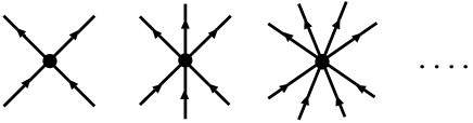
In this section, we consider the -corrections which generate -body interaction as shown in Fig. 1. Then the model can not be solved exactly anymore. What we can do is to perform a perturbative expansion in terms of . First of all, we give a scaling argument and justify our perturbative approach in the next subsection.
A Renormalization group argument
We consider correlation effects beyond the mean field solution given by , eq.(16). We apply the scaling transformation which keeps , eq.(16), invariant,[23]
| (22) | |||||
| (23) |
Then, the scaling dimension of reads . Now we consider the scaling equation for the effective coupling of (), . Applying the perturbative renormalization group argument, we obtain the scaling equation,
| (24) |
Here is the dimensionless scaling parameter which goes to infinity in the low-energy limit, and is the scaling dimension of . Although we know the value of for the 1D Hubbard model from the conformal field thoery argument,[20, 21] in may show a deviation from the critical power law behavior in the long-distance limit owing to the deformation of the Fermi surface discussed above. In the conventional Ginzburg-Landau arguments of coupled chains,[24] it is often assumed that the coefficient of the fourth order term is a non-zero constant. This means . However the concrete value of does not matter in the following argument. We just assume it is finite. Then we can easily see that for , with is irrelevant in the low-energy state, and can be treated perturbatively. The existence of the critical dimension for the irrelevance of means nothing more than the stability of the RPA like mean field solution in the large dimensional system with the long-range inter-chain interaction, which is consistent with the common sense that a mean field solution is more stabilized in the presence of long-range interaction in spatial dimension larger than an upper critical dimension. In this paper, we consider the infinitely large which simplifies the perturbative calculation as well as ensures the controllable expansion. In this limit, the self-energy does not depend on the transverse momentum , as in the case of the infinitely large dimensional Hubbard model, where the self-energy is a completely local quantity.[25, 26]
In the following, we investigate strong correlation effects by performing the perturbative calculation in Before doing that, we need to care about any possibility of spontaneous symmetry breaking such as magnetic transition which may be brought about by the interaction between quasiparticles. However, in this paper, we assume that no spontaneous symmetry breaking occurs before the MH transition, since we are concerned with correlation effects in the Fermi liquid state near the paramagnetic MH transition point.
Before carrying out the perturbative calculation, we would like to make a comment about the Luttinger’s theorem which holds for the case of finite . The change of the Fermi surface volume due to the Fermi surface shift, eq.(13), is given by . In the case of , we have,
| (25) |
where
| (26) |
Thus the Fermi surface volume is preserved. This is consistent with the Luttinger’s theorem.
B Perturbative calculation of the self-energy
We evaluate the -corrections to the self-energy. We neglect the diagrams which just give a chemical potential shift, as shown in Fig. 2(a),(b),(c). The diagram of order (Fig. 2(d)) is most important for the mass enhancement factor. The self-energy correction from this diagram is given by,
| (27) |
The next order diagram which contributes to the mass enhancement factor is of order (Fig. 2(e)), since as seen from eq.(24). It is evaluated as,
| (28) |
Note that shows more singular -dependence than . Higher order corrections also give more singular -dependence. Thus we need to be careful with the applicability of our perturbative calculation. According to eq.(24), . Then, the ratio of eq.(28) to eq.(27) is sufficiently small provided that . The applicability of the result of order , (27), is restricted to this low-energy scale. In other words, as the electron density approaches the half-filling , the energy range where eq.(27) can be used becomes very narrower such as . In the following, we restrict our argument to this energy range.
C Specific heat coefficient
Using eq.(27) we have the mass renormalization factor,
| (29) |
The quasiparticle weight is much more suppressed compared to eq.(17). In contrast, the quasiparticle damping is still infinitesimally small in the low-energy state. Thus the Fermi liquid theory is applicable even in the vicinity of the MH transition. We obtain the -dependence of the specific heat coefficient,[27]
| (30) |
The specific heat coefficient shows the divergent behavior as decreases. The mass enhancement is larger than that of the non-interacting limit obtained in §2. Note that the exponent of eq.(30) depends on the strength of interaction indicating the non-universal behavior.
D Single-particle density of states
Up to the second order corrections in , the single-particle density of states at the Fermi surface is given by,
| (31) |
The result is the same as that obtained in §2(eq.(21)). Higher-order corrections does not affect this result, as expected from the conventional Fermi liquid theory.
E Drude weight
In the computation of the Drude weight, we take into account the effect of the velocity renormalization, due to the self-energy correction, eq.(27), as well as the vertex corrections to electric currents which is nothing but the back flow effect,[28]
| (32) |
Here is the interaction between the quasiparticles with momenta and . When we calculate the current vertex corrections, we generally need to pay attention to the charge conservation law. However the charge conservation is not trivial in our system. The non-perturbed state obtained in §2 is composed of the Fermi liquid part and the Luttinger liquid part. As a result, the weight of the Fermi liquid part may be transfered to the Luttinger liquid part by the interaction introduced in this section. The charge conservation law is not expressed in the closed form only in the Fermi liquid part. Thus, here, we just evaluate the vertex corrections up to the second order in , of which the diagrams are shown in Fig. 3. Note that each line in Fig.3 is the renormalized single-particle Green’s function with the quasiparticle weight , eq. (29). This renormalization effect must be taken into account, because the use of the bare propagator eq.(11) for the calculation of the diagrams in Fig. 3 leads to unphysical enhancement of current vertex corrections for small . This treatment may be justified by the Ward-Takahashi identity, though we do not discuss this point furthermore because of the reason mentioned above. Then we have the Drude weight,
| (33) |
It is noted that the relation, -independent still holds approximately. This is because that the corrections due to the back flow effect is sub-leading in this systems in the vicinity of the MH transition and thus the leading behavior of the Drude weight is determined by the velocity of quasiparticles.
F Compressibility
Here we will see that the effect of the interaction between quasiparticles affects the -dependence of the compressibility drastically. Using the dressed single-particle Green’s function with the mass renormalization factor , as in the case of the Drude weight, we compute the lowest order diagram for the compressibility as shown in Fig. 4(a),
| (34) |
Higher order diagrams shown in Fig. 4(b) give sub-dominant contributions for small .
In contrast to the result in §2, as , decreases toward zero, though we can not reach the half-filling point, , because of the restriction . In the conventional Fermi liquid theory, it is expected that vertex corrections due to electron-electron interaction suppress the compressibility. However, here, the lowest order bubble diagram Fig. 4(a) gives the strong suppression of the compressibility. This implies that the usual Fermi liquid effect of vertex corrections may be incorporated effectively into the mass renormalization factor in our model. The drastic change of -dependence due to -corrections means that terms, eq.(9), are in a sense dangerously irrelevant for .
IV Effects of Disorder: a Possibility of Mott Glass
In this section, we study the effects of random potential in the vicinity of the Mott transition. We are mainly concerned with a possible realization of the Mott glass state proposed by Orignac et al.[14] The Mott glass state is characterized by vanishing compressibility and the dynamical conductivity which obeys the Mott’s law, namely, for small . In this state, although a single-particle exciation has a charge gap, particle-hole excitation is gapless showing the characteristic behavior of Anderson localization. Thus the Mott glass state is regarded as an intermediate state between Mott insulator and Anderson localization. This state is similar to Anderson localized state in the presence of long-range Coulomb interaction in the spatial dimension larger than 2.[29] However the Mott glass state is realized for the case of finite-range interaction and even for 1D systems. To see a possible realization of this state, we add the disorder potential term to the Hamiltonian:
| (35) |
Here is a random potential. In the presence of disorder, we can derive the effective action in a simalr way to that applied for clean systems. Using the Hubbard-Stratonovich transformation,
| (36) | |||||
| (37) |
we decouple the disorder term as well as the transverse hopping term. Then integrating out , fields, we have,
| (38) | |||
| (39) | |||
| (40) | |||
| (41) | |||
| (42) | |||
| (43) |
Since our model has the infinite , Anderson localization in the transverse direction does not occur. For this reason, we concentrate on effects of disorder only in the direction parallel to the chains, and consider randomness without spatial dependence in the transverse direction, namely,
| (44) | |||||
| (45) |
This assumption simplifies the following argument substantially. Moreover we consider sufficiently small disorder to stabilize the single-particle charge gap. It is known that the Mott-Hubbard gap of the 1D Hubbard model is not collapsed by sufficiently small disorder.[16, 17, 18] In the following, we take into account only the backward scattering due to random potential and neglect the forward scattering which is not important for the realization of the Mott glass. Using the renormalization group argument similar to that developed in §3.1, we can easily show that of eq.(42) are irrelevant in the low energy state. Thus we neglect the disorder effects of , and take into account the lowest order corrections in as done in §3. Then, we have the low energy effective action,
| (46) |
In the following, we neglect the irrelevant interactions of this action. As a result, the model is equivalent to the 1D disordered non-interacting fermion system, which has been studied extensively so far.[30, 31] However the important difference from the classical model is that the effects of electron correlation are incorporated into the mass renormalization factor and the renormalized Fermi velocity . Following Berezinskii,[30] and Abrikosov and Ryzhkin,[31] we can caluculate the dynamical conductivity. The result is given by,
| (47) |
This expression shows the Mott’s law, indicating the Anderson localized state. For small , it behaves like,
| (48) |
For the 1D Hubbard model, . Thus as , it is expected that vanishes, though we can not reach because of the reason mentioned in the previous sections. In this case, the Mott glass state may not realize at half-filling. However in the presence of a finite range interaction, such as next-nearest or next-next-nearest intearction, it is possible to be for . It is noted that even for , the single-particle Green’s function, eq.(11) still has a quasiparticle pole. Moreover the velocity of holon near the half-filling point behaves like even in the presence of a finite-range interaction provided that the low-energy effective theory of the single chain is given by Sine-Gordon model. Thus the argument presented in the previous sections is applicable. Then, in this case, there is a possibility of the Mott glass state with for . This result is consistent with the physical intuition that the presence of a finite-range interaction reduces particle-hole excitation energy lower than a single-particle excitation energy, stabilizing the Mott glass state. Since our approach breaks down just at the half-fillig, the above result is not a direct evidence of the Mott glass state. However it implies a strong possibility of its realization at half-filling.
V Summary and Discussion
We have studied strong correlation effects of the Fermi liquid state near the MH transition in the quasi-one-dimensional Hubbard model. We have treated the intra-chain electron correlation exactly exploiting the exact results of the Bethe ansatz solution. The systematic perturbative expansion in terms of the inverse of the transverse hopping range has been used for the analysis of the inter-chain electron correlation effects. It has been shown that the precursor of the MH transition can be seen in the -dependence of the Drude weight, the specific heat coefficient, and the compressibility, and that the exponents which depend on the strength of electron-electron interaction characterize non-universal behaviors of the MH transition. We have also studied effets of disorder on this strongly correlated state. We otain the dynamical conductivity which obeys the Mott’s law. The result implies a possible realization of the Mott glass state at half-filling.
In real systems, the situation with a large hardly realizes. We would like discuss about to what extend our results are valid in systems with small . In principle, we can incorporate the finiteness of by the systematic expansion. As shown in §3, if we take into account the second-order self-energy corrections, we have the Fermi liquid state with a strongly renormalized quasi-particle weight, and then near half-filling, higher order corrections in are much suppressed. (see the calculation of the Drude weight and the compressibility in §3.) Thus it is expected that the physical picture of weakly-interacting quasi-particles with a strongly renormalized mass may be hold in the vicinity of the Mott transition even for the case with small , though the exponents of physical quantities should be quantatively changed from those obtained in §3.
As claimed in §2., the applicability of our results is restricted to . Thus, unfortunately, we can not reach the half-filling point. We need the information for off-critical behaviors of correlation functions of the 1D Hubbard model to investigate the case of . Recently, the substantial progress of the study of correlation functions of 1D massive integrable models has been achieved.[32] It may be possible to apply the new technique for the case of . We would like to address this issue in the near future.
Acknowledgment
The author would like to thank N. Kawakami and K. Yamada for invaluable discussions. This work was partly supported by a Grant-in-Aid from the Ministry of Education, Science, Sports and Culture, Japan.
REFERENCES
- [1] N. F. Mott, Philos. Mag. 6 (1961) 287.
- [2] J. Hubbard, Proc. R. Soc. London Ser A 281 (1964) 401.
- [3] W. F. Brinkman and T. M. Rice, Phys. Rev. B2 (1970) 4302.
- [4] For a review see, for example, N. F. Mott, Metal-Insulator Transitions (Taylor and Francis, London, 1990); F. Gebhard, The Mott Metal-Insulator Transition (Springer, Berlin, 1997); M. Imada, A. Fujimori, and Y. Tokura, Rev. Mod. Phys. 70 (1998) 1039, and references therein.
- [5] E. Lieb and F. W. Wu, Phys. Rev. Lett. 20 (1968) 1445.
- [6] N. Kawakami and S.-K. Yang, Phys. Rev. Lett.65 (1990) 3063.
- [7] H. J. Schulz, Phys. Rev. Lett.64 (1990) 2831.
- [8] T. Usuki, N. Kawakami, and A. Okiji, J. Phys. Soc. Jpn. 59 (1990) 1357.
- [9] M. J. Rozenberg, X. Y. Zhang, and G. Kotliar, Phys. Rev. Lett. 69 (1992) 1236; X. Y. Zhang, M. Rozenberg, and G. Kotliar, ibid. 70 (1993) 1666; G. Moeller, Q. Si, G. Kotliar, M. Rozenberg, and D. S. Fisher, Phys. Rev. Lett. 74 (1995) 2082.
- [10] For a review see A. Georges, G. Kotliar, W. Krauth, and M. J. Rozenberg, Rev. Mod. Phys. 68 (1996) 13, and references therein.
- [11] X. G. Wen, Phys. Rev. B42 (1990) 6623.
- [12] D. Boies, C. Bourbonnais, and A.-M.S. Tremblay, Phys. Rev. Lett. 74 (1995) 968.
- [13] The model with the infinitely large was also studied in connection with the issue of crossover between Fermi liquid and Luttinger liquid in A. M. Tsvelik, cond-mat/9607209, and in E. Arrigoni, Phys. Rev. Lett. 83 (1999) 128; cond-mat/9910114.
- [14] E. Orignac, T. Giamarchi, and P. Le Doussal, Phys. Rev. Lett. 83 (1999) 2378.
- [15] R. Shankar, Int. J. Mod. Phys. B4 (1990) 2371.
- [16] S. Fujimoto and N. Kawakami, Phys. Rev. B54 (1996) 11018.
- [17] M. Mori and H. Fukuyama, J. Phys. Soc. Jpn. 65 (1996) 3604.
- [18] Y. Otsuka, Y. Morita and Y. Hatsugai, Phys. Rev. B58 (1998) 15314.
- [19] F. D. M. Haldane, Phys. Rev. Lett. 45 (1980) 1358; ibid. 47 (1981) 1840; J. Phys. C 14 (1981) 2585.
- [20] N. Kawakami and S.-K. Yang, Phys. Lett. 148A (1990) 359.
- [21] H. Frahm and V. E. Korepin, Phys. Rev. B42 (1990) 10553.
- [22] E. Müller-Hartmann, Z. Phys. B76 (1989) 211.
- [23] see, for example, R. Shankar, Rev. Mod. Phys. 66 (1994) 129; T. Chen, J. Fröhlich, and M. Seifert, in Fluctuating Geometries in Statistical Mechanics and Field Theory ed. F. David, P. Ginsparg and J. Zinn-Justin (North-Holland, Amsterdam, 1996).
- [24] D. J. Scalapino, Y. Imry, and P. Pincus, Phys. Rev. B11 (1975) 2042.
- [25] W. Metzner and D. Vollhardt, Phys. Rev. Lett. 62 (1989) 324; For a review see D. Vollhardt, in Correlated Electron Systems. ed. V. E. Emery (World Scientific, Singapore, 1990).
- [26] E. Müller-Hartmann, Z. Phys. B74 (1989) 507.
- [27] J. M. Luttinger, Phys. Rev. 119 (1960) 1153.
- [28] P. Nozières, Interacting Fermion Systems (Benjamin, 1964).
- [29] A. L. Efros, J. Phys. C9 (1976) 2021.
- [30] V. L. Berezinskii, Soviet Phys. JETP 38 (1974) 620.
- [31] A. A. Abrikosov and I. A. Ryzhkin, Adv. in Phys. 27 (1978) 147.
- [32] S. Lukyanov, Commun. Math. Phys. 167 (1995) 183; Phys. Lett. B325 (1994) 409.